Article

Computing the Gromov-Wasserstein Distance between Two Surface Meshes Using Optimal Transport

1
Department of Computer Science, University of California, Davis, CA 95616, USA
2
Institut Pasteur, Université Paris-Cité and CNRS, UMR 3528, Unité Architecture de Dynamique des Macromolécules Biologiques, 75015 Paris, France
3
Institut de Physique Théorique, CEA, CNRS, Université Paris-Saclay, 91191 Gif-sur-Yvette, France
*
Author to whom correspondence should be addressed.
Algorithms 2023, 16(3), 131; https://doi.org/10.3390/a16030131
Submission received: 19 January 2023 / Revised: 20 February 2023 / Accepted: 25 February 2023 / Published: 28 February 2023
(This article belongs to the Topic Mathematical Modeling in Physical Sciences)

Abstract

:
The Gromov-Wasserstein (GW) formalism can be seen as a generalization of the optimal transport (OT) formalism for comparing two distributions associated with different metric spaces. It is a quadratic optimization problem and solving it usually has computational costs that can rise sharply if the problem size exceeds a few hundred points. Recently fast techniques based on entropy regularization have being developed to solve an approximation of the GW problem quickly. There are issues, however, with the numerical convergence of those regularized approximations to the true GW solution. To circumvent those issues, we introduce a novel strategy to solve the discrete GW problem using methods taken from statistical physics. We build a temperature-dependent free energy function that reflects the GW problem’s constraints. To account for possible differences of scales between the two metric spaces, we introduce a scaling factor s in the definition of the energy. From the extremum of the free energy, we derive a mapping between the two probability measures that are being compared, as well as a distance between those measures. This distance is equal to the GW distance when the temperature goes to zero. The optimal scaling factor itself is obtained by minimizing the free energy with respect to s. We illustrate our approach on the problem of comparing shapes defined by unstructured triangulations of their surfaces. We use several synthetic and “real life” datasets. We demonstrate the accuracy and automaticity of our approach in non-rigid registration of shapes. We provide numerical evidence that there is a strong correlation between the GW distances computed from low-resolution, surface-based representations of proteins and the analogous distances computed from atomistic models of the same proteins.

1. Introduction

In 1776, Gaspard Monge presented an intriguing problem to the French Academy of Science [1]. Consider two domains D 1 and D 2 in the plane. D 1 (referred to as “déblai” by Monge) contains an excess of earth that needs to be transported to D 2 (“remblai” in Monge’s terminology). Assuming that the earth at a point ( x , y ) in D 1 is transported to a position F ( x , y ) in D 2 , and that the masses associated with the point and image are equal, proportional to d x d y , the total “cost” C of the transportation is given by
C = D 1 | | ( x , y ) F ( x , y ) | | d x d y ,
where | | . | | stands for the distance in the plane. Finding the minimum cost for moving the earth is then akin to finding this transport function F. Monge acknowledged in his presentation that he had not solved this problem on a practical level. This “allocation of ressources” problem became well known, however, reappearing in many disciplines and consequently has been the object of many studies. Erwin Schrödinger, for example, expressed it as the problem of finding how to evolve a probability distribution into another (see [2] for a review), the Schrödinger bridge problem. Kantorovich relaxed the Monge problem by allowing masses to split [3]. He also formulated a method, linear programming, for solving his relaxed version. All these problems are now referred to as the optimal transport problems, or OT. The OT problem is particularly intriguing since its solutions involve two crucial elements. It first specifies a distance between the measured spaces taken into account. This distance is known as the Monge-Kantorovich distance, the Wasserstein distance, or the earth mover’s distance, according to the field of applications. It also derives the optimal transport plan between the measured spaces, thereby defining a registration between the spaces. Consequently, applications of OT have exploded in the recent years (for in-depth reviews of OT and its uses, see [4,5]).
The Monge-Kantorovich OT problem can be formulated as follows. Let A and B be two subsets of a space M with a metric d, and let α and β be probability measures on A and B, respectively. Let C be a cost function C : A × B R + . The objective is to find a coupling G on A × B that minimizes a transportation cost U defined as
U ( G ) = A B C ( a , b ) G ( a , b ) d ( a , b ) .
The minimum of U ( G ) is to be identified over the couplings G that satisfy the following constraints on their restrictions to the subsets A and B:
a , B G ( a , b ) d b = α ( a )
b , A G ( a , b ) d a = β ( b ) .
It was shown that this minimum exists and that it defines a distance between the two probability measures α and β that satisfies all metric properties [6].
One key condition for solving the optimal transport problem between two sets A and B is that those sets belong to the same metric space. This allows for the definition of a distance between any point of A and any point of B, and therefore of a cost function between the two sets. In practice, however, the two sets may not be in the same metric space, or, even if they do, the corresponding metric may not be practical. Consider for example two sets of points in R 3 ; while it is possible to compute the euclidean distance between any pairs of points belonging to the two sets, inter distances between the two sets depend on the relative position of the two sets, namely a rigid body transformation involving six real-valued parameters (three that define a rotation, three that define a translation). Distances within each set are independent of such transformation; such distances, however, define a different metric space, one for each set of points. Several methods have been developed to use this information within the framework of optimal transport [7,8,9]. Here we are concerned with the Gromov-Wasserstein formalism [8], which has become popular for shape matching [8], for word embedding [10], as well as in the machine learning community, solving learning tasks such as heterogenous domain adaptation [11], deep metric alignment [12], computing distances between graphs [13] and graph classification [14,15], clustering [16] or generative modeling [17], among others. The GW problem can be stated as follows. Let ( A , d A ) and ( B , d B ) be two metric spaces, and let α and β be probability measures on A and B, respectively. The goal is to find a coupling G on A × B that minimizes the transport cost T defined as
T p ( G ) = A × A B × B G ( a , b ) d A ( a , a ) d B ( b , b ) p G ( a , b ) d a d a d b d b 1 p ,
with p 1 (the most common value for p is 2, as it will be discussed below). The minimum of T p ( G ) is to be found over couplings that satisfy the constraints defined in Equation (3). As for the standard Monge-Kantorovich OT presented above, it was proved that a minimum to the transport cost defined in Equation (4) always exists [8]; we write this minimum as G W p ( α , β ) . Finding this minimum, however, is a quadratic optimization problem, as opposed to finding the coupling that minimizes the transport cost associated with the OT problem (Equation (2)), which is a linear optimization problem. This minimum of the transportation cost defines a distance over the space of metric measured spaces (i.e., the triplet ( A , d A , α ) ) modulo the measure-preserving isometries [8]. When the metrics d A and d B are the Euclidean distance over real numbers, i.e., when A = R m and B = R n (with n not necessarily equal to m), and d A = | | . | | R m and d B = | | . | | R n (where | | . | | means the Euclidean norm), and when p = 2 , an interesting property of G W 2 ( α , β ) is that it is invariant with respect to rigid body transformations (i.e., isometries). This is of significance for example if the GW framework is to be used to compare shapes in space, when this comparison has to be independent of the relative positions of the shapes..
As mentioned above, classical OT is a linear programming problem. It is intriguing, however, that the current successes of OT are not due to recent advances in solving LP problems. They were instead prompted by the idea of entropic regularization, namely minimizing a modified version of the transport cost defined in Equation (2):
U ϵ ( G ) = U ( G ) ϵ H ( G ) ,
where ϵ is the parameter that controls the amount of regularization and H ( G ) is an entropy on the coupling G. It is there to impose the positivity of its elements [18]. As ϵ 0 the regularized problem tends to the traditional problem. Interestingly, the minimum of the regularized transport cost U ϵ ( G o p t ) is a distance that satisfies all metric properties for all values of ϵ . This distance is called the Sinkhorn distance [18]. The main advantage of the entropic regularization is that it leads to a strictly convex problem that has a unique solution [18]. In addition, this solution can be found effectively using the Sinkhorn’s algorithm [19,20,21]. Sinkhorn’s algorithms have running times of order O ( N 2 ) , while solving directly the OT problem as a linear program problem has a running time complexity of O ( N 3 ) .
The same entropic regularization can be used the solve the GW problem, originally a quadratic optimization problem which is NP-hard in its general formulation. The idea is the same as for OT, namely add a regularized term to Equation (4) (see [22]):
T p , ϵ ( G ) = T p ( G ) p ϵ H ( G ) .
Note that here it is not T p ( G ) that is considered, but its p-th power. While this simplifies the optimization process, it sets T p , ϵ ( G ) to be a “discrepancy” (in the language of Peyré et al. [22]) and not a distance with metric properties. The addition of the entropic regularization led, however, to an iterative algorithm for finding the GW discrepancy, with each iteration amounting to solve a regularized OT problem [22].
While the regularization based on entropy significantly expanded the appeal of OT, there are issues with the numerical convergence of the regularized solution to the actual OT solution. Furthermore, the physical significance of this regularization is unclear, despite its reference to entropy. Using methods from statistical physics, we have recently designed a novel framework for solving the OT problem that alleviate those issues [23,24]. The main idea is to build a strongly concave temperature dependent effective free energy function that encapsulates the constraints of the OT problem. The maximum of this function is proved to define a metric distance in the space of measured sets of points of fixed cardinality for all temperatures. In addition, this distance is proved to decrease monotonically to the regular OT distance at zero temperature. This property enables a robust algorithm for finding the OT distance using temperature annealing. This approach has been adapted to solving the assignment, or Monge problem [25], as well as to the unbalanced optimal transport problem [26]. In this paper we adapt it to solving the GW problem.
The paper is structured as follows. In the next section, we introduce the GW problem and its regularized version for discrete metric measured spaces. The following section covers the specifics of the statistical physics method we propose. All proofs of important properties of this method are given in the appendices. The subsequent section is devoted to the algorithm that implements our method in a C++ program, FreeGW. Next, we present numerical applications to the problem of comparing and registering 3D shapes, using examples based on synthetic data as well as on real data. The conclusion highlights possible future developments.

2. The Discrete Gromov-Wasserstein Problem

This section briefly describes the discrete Gromov Wasserstein transport problem and its regularized version. More thorough descriptions can be found in Refs. [7,8,22].
The discrete version of the GW problem is an optimal transport problem between two discrete probability measures whose supports are metric spaces ( M 1 , d 1 ) and ( M 2 , d 2 ) with possibly different metrics. Let S 1 and S 2 be subsets of M 1 and M 2 with cardinality N 1 and N 2 , respectively. Each point k in S 1 (resp S 2 ) is characterized by a “mass” m 1 ( k ) (resp m 2 ( k ) ). We assume balance, namely that k m 1 ( k ) = l m 2 ( l ) . In the following, these sums are set to 1, but the formalism could easily be adapted to handle a different values.
The discrete GW problem is defined as finding a coupling or transport plan G that minimizes the total transport cost U defined as
U p ( G ) = k , l k , l G ( k , l ) d 1 ( k , k ) d 2 ( l , l ) p G ( k , l ) ,
where p is a fixed integer greater or equal to 1, and the summations extend over all ( k , k ) S 1 2 and ( l , l ) S 2 2 . Note that G is a matrix of correspondence between points k in S 1 and points l in S 2 . The minimization is to be performed over those matrices G that satisfy the following constraints
( k , l ) , G ( k , l ) 0 ,
k , l G ( k , l ) = m 1 ( k ) ,
l , k G ( k , l ) = m 2 ( l ) .
The set of all matrices G for which those conditions (8) are satisfied defines a polytope, which we refer to as G ( S 1 , S 2 ) .
The minimization of the cost U p ( G ) yields an optimal transport plan G o p t . We refer to the minimum of the cost as d p ( S 1 , S 2 ) . Note that d p ( S 1 , S 2 ) is not a distance. Its p-root, however, which we write as G W p ( S 1 , S 2 ) = U p ( G o p t ) 1 p is a metric distance between ( S 1 , d 1 ) and ( S 2 , d 2 ) quotiented by measure-preserving isometries [8].
Solving for the transport plan that minimizes Equation (7) under the constraints defined in Equation (8) is a non-convex quadratic optimization problem [27,28] and therefore N P -hard in the general case (see for example [29]). To circumvent this large computing cost when N is large, following Cuturi’s idea proposed for the optimal transport problem [18], Peyré et al. proposed a regularized version of Equation (7) [22]:
U p , ϵ ( G ) = k , l k , l G ( k , l ) d 1 ( k , k ) d 2 ( l , l ) p G ( k , l ) + ϵ k , l G ( k , l ) log ( G ( k , l ) ) ,
where ϵ is a parameter that controls the level of regularization. This parameter scales an entropic term, with the entropy set to x ln ( x ) , the standard information theory entropy, which imposes the positivity of the G ( k , l ) terms [18]. This regularized GW problem can then be solved iteratively using a regularized linear optimal transport solver, as described in Algorithm 1.
Algorithm 1 is akin to a sequential quadratic programming method [30]. Briefly, given two sets of weighted points and the intra-set distances between those points, a “cost matrix” between the two sets is defined from the current transport plan G (initialized according to the masses of the points). This cost matrix is then used to solve a regularized linear optimal transport problem. The corresponding optimal transport plan is then used to update the cost matrix, and the procedure is then iterated until the transport plan does not change anymore (within a tolerance), i.e., when the transport plan and the cost matrix are consistent. There are many options to solve the regularized linear optimal transport problem in step 2, such as the Sinkhorn algorithm [20,21] initially proposed for solving the OT problem by Cuturi [18], or stabilized version of this algorithm [31,32,33,34,35], or using our own method based on statistical physics [23,24].
Algorithm 1 An iterative solver for the regularized GW problem.
  • Input:  N 1 and N 2 , the size of the two sets of points S 1 and S 2 . The mass vectors m 1 ( k ) and m 2 ( l ) , for k [ 1 , N 1 ] and l [ 1 , N 2 ] . The distance matrices d 1 ( k , k ) and d 2 ( l , l ) over all points ( k , k ) S 1 2 and ( l , l ) S 2 2 . Tolerance, TOL; regularization parameter, ϵ ; N, maximum number of iterations.
  • Initialize: Initialize transport plan G 0 ( k , l ) = m 1 ( k ) m 2 ( l )
  • for  n = 1 , , N   do
  •     (1) Define “cost matrix” C n ( k , l ) = k = 1 N 1 l = 1 N 2 d 1 ( k , k ) d 2 ( l , l ) p G n 1 ( k , l ) .
  •     (2) Solve G n = argmin G U ( G ) = argmin G k , l C n ( k , l ) G ( k , l ) + ϵ k , l G ( k , l ) log ( G ( k , l ) ) under the constraints defined in Equation (8).
  •     (3) If | | G n G n 1 | | < T O L , break.
  • end for
  • Output: The optimal transport plan, G n .
Algorithm 1 can be seen as applying successive linear approximation to the quadratic GW problem and as such it is expected to be efficient in computing time. There remains difficulties, however, as:
(i)
Solving the regularized OT problem in step 2 is difficult when ϵ 0 (a necessary condition to get to the real GW distance).
(ii)
Algorithm 1 is basically a fixed point method for which there is no guarantee of convergence. This is discussed in detail in Ref. [22].
(iii)
There is no easy option within Algorithm 1 to compute a scaling factor between distances within S 1 and distances within S 2 . Those distances may have different scales, however, which can significantly impact the numerical stability of the algorithm.
In the following section, we describe a different method for solving the GW problem that attempt to solve at least some of these concerns.

3. A Statistical Physics Approach to Solving the Gromov-Wasserstein Problem

Solving the GW problem amounts to finding the minimum of a function defined by Equation (7) over the space of possible couplings between the two discrete sets of points considered. If this function is reworded as an “energy”, statistical physics allows for a different perspective on how to solve this problem. Indeed, in statistical physics, finding the minimum of an energy function is equivalent to finding the most probable state of the system it characterizes. Here, this system corresponds to the different couplings between between the measured sets of points S 1 and S 2 . We refer to the space of such couplings G ( S 1 , S 2 ) (see above). Couplings G in this space satisfy multiple constraints. Their row sums and row columns correspond to the masses associated with S 1 and S 2 , respectively (see Equation (8)). In addition, their elements are positive, and in fact smaller than one, if we assume that the sums of the masses on S 1 and on S 2 are both equal to 1 (the fact that these sums are equal is referred to as the balance condition and setting them to 1 is arbitrary but useful, as illustrated below).
A state in this system is then characterized with a coupling G and its energy value U p ( G ) as defined by Equation (7). To account for possible differences of scales between the metrics on S 1 and S 2 , we introduce a scaling factor s between the distances d 1 and d 2 :
U p ( s , G ) = k , l k , l G ( k , l ) d 1 ( k , k ) s · d 2 ( l , l ) p G ( k , l ) ,
where p is a constant and s is considered as a variable. The probability of finding the system in a state characterized by G and s is:
P ( s , G ) = 1 Z β ( s , S 1 , S 2 ) e β U p ( s , G ) .
In this equation, β is the inverse of the temperature, namely β = 1 / ( k B T ) with k B the Boltzmann constant and T the temperature. Z β ( s , S 1 , S 2 ) is the partition function defined as
Z β ( s , S 1 , S 2 ) = G G ( S 1 , S 2 ) e β U p ( s , G ) d μ 12 .
An interesting property of a partition function Z is that most thermodynamic variables of the system can be expressed as functions of Z, or as functions of its derivatives. This is the case for the free energy of the system:
F β ( s , S 1 , S 2 ) = 1 β ln ( Z β ( s , S 1 , S 2 ) ) ,
as well as for the average energy E β ( s , S 1 , S 2 ) = < U p ( s , G ) > s R , G G by
E β ( s , S 1 , S 2 ) = ln ( Z β ( s , S 1 , S 2 ) ) β .
In addition to finding the coupling matrix G, we want to find the scaling factor s that defines the best match between the two distributions. To reach this goal, we will minimize the free energy F β ( s , S 1 , S 2 ) with respect to s. The minimized free energy is denoted by F β ( S 1 , S 2 ) and similarly, the average energy computed with the minimal s is denoted as E β ( S 1 , S 2 ) .
We start with an important property of the free energy and of the average energy:
Proposition 1.
For all β > 0 , the free energy and the average energy are monotonically decreasing functions of β. Both functions converge to d p ( S 1 , S 2 ) from which we can compute the GW distance as G W p ( S 1 , S 2 ) = d p ( S 1 , S 2 ) 1 p .
Proof. 
How the functions F β and of E β behave as the parameter β is increased is studied in Appendix A.    □
This approach to solving the GW problem is appealing. It is based on a temperature-dependent free energy with a monotonic dependence on the inverse of the temperature, β , and convergence to the actual GW distance at zero temperature. In practice, however, it is of limited interest because the partition function and thus the extrema of the free energy cannot be computed explicitly. We propose using the saddle point approximation to approximate these quantities. We will demonstrate that the corresponding mean field values have the same properties as the exact quantities defined above. These mean field values are easily calculated.
Following the method described in Ref. [23] to impose the constraints that define G ( S 1 , S 2 ) , the partition function can be rewritten as
Z β ( s , S 1 , S 2 ) = 0 1 k , l d G ( k , l ) e β k , l k , l G ( k , l ) d 1 ( k , k ) s · d 2 ( l , l ) p G ( k , l ) × k δ l G ( k , l ) m 1 ( k ) l δ k G ( k , l ) m 2 ( l ) .
To account for the quadratic term in the exponential, we introduce new variables C ( k , l ) that are constrained to mimic a cost function between S 1 and S 2 :
Z β ( s , S 1 , S 2 ) = 0 1 k , l d G ( k , l ) + k , l d C ( k , l ) e β k , l G ( k , l ) C ( k , l ) × k δ l G ( k , l ) m 1 ( k ) l δ k G ( k , l ) m 2 ( l ) k , l δ k , l d 1 ( k , k ) s · d 2 ( l , l ) p G ( k , l ) C ( k , l ) .
Using the Fourier representation of a delta function,
δ ( x ) = 1 2 π + e i x t d t ,
the partition function can be recast with integrals only. To do so, we introduce the Fourier variables D ( k , l ) , λ ( k ) and μ ( l ) , with ( k , l ) [ 1 , N 1 ] × [ 1 , N 2 ] . Omitting the normalization factors 1 / ( 2 π ) , the partition function can then be expressed as,
Z β ( s , S 1 , S 2 ) = + k , l d C ( k , l ) 0 1 k , l d G ( k , l ) e β k , l C ( k , l ) G ( k , l ) × + k d λ ( k ) e i β k , l λ ( k ) G ( k , l ) + i β k λ ( k ) m 1 ( k ) + l d μ ( l ) e i β k , l μ ( l ) G ( k , l ) + i β l μ ( l ) m 2 ( l ) + k , l d D ( k , l ) e i β k , l D ( k , l ) C ( k , l ) i β k , l D ( k , l ) k , l d 1 ( k , k ) s · d 2 ( l , l ) p G ( k , l ) .
Note that we have introduced an explicit scaling factor β for the variables D ( k , l ) , λ ( k ) and μ ( l ) . The corresponding terms are then consistent with the energy term. Note also that the terms within the integrals in Z are now complex functions, while the partition function Z itself is real. For sake of clarity, we include the i in D ( k , l ) , λ ( k ) and μ ( l ) , i.e., D ( k , l ) i D ( k , l ) , λ ( k ) i λ ( k ) and μ ( l ) i μ ( l ) . Those variables are now complex.
After rearrangements,
Z β ( s , S 1 , S 2 ) = + d C ( k , l ) + d D ( k , l ) + k d λ ( k ) + l d μ ( l ) e β k , l C ( k , l ) D ( k , l ) + k λ ( k ) m 1 ( k ) + l μ ( l ) m 2 ( l ) 0 1 k , l d G ( k , l ) e β k , l G ( k , l ) ( C ( k , l ) + λ ( k ) + μ ( l ) + k , l d 1 ( k , k ) s · d 2 ( l , l ) p D ( k , l ) ) .
Shifting C ( k , l ) C ( k , l ) + k , l d 1 ( k , k ) s · d 2 ( l , l ) p D ( k , l ) ,
Z β ( s , S 1 , S 2 ) = + d C ( k , l ) + d D ( k , l ) + k d λ ( k ) + l d μ ( l ) e β k , l C ( k , l ) D ( k , l ) + k λ ( k ) m 1 ( k ) + l μ ( l ) m 2 ( l ) e β k , l k , l D ( k , l ) d 1 ( k , k ) s · d 2 ( l , l ) p D ( k , l ) 0 1 k , l d G ( k , l ) e β k , l G ( k , l ) ( C ( k , l ) + λ ( k ) + μ ( l ) ) .
We can now perform the integration over the real variables G ( k , l ) to get
Z β ( s , S 1 , S 2 ) = + d C ( k , l ) + d D ( k , l ) + k d λ ( k ) + l d μ ( l ) e β k , l C ( k , l ) D ( k , l ) + k λ ( k ) m 1 ( k ) + l μ ( l ) m 2 ( l ) e β k , l k , l D ( k , l ) d 1 ( k , k ) s · d 2 ( l , l ) p D ( k , l ) k , l 1 e β C ( k , l ) + λ ( k ) + μ ( l ) β C ( k , l ) + λ ( k ) + μ ( l ) .
We rewrite this partition function as
Z β ( s , S 1 , S 2 ) = + d C ( k , l ) + d D ( k , l ) + k d λ ( k ) + l d μ ( l ) e β F β ,
where F β is the effective free energy defined by:
F β = k , l D ( k , l ) C ( k , l ) k λ ( k ) m 1 ( k ) + l μ l m 2 ( l ) + k , k l , l D ( k , l ) d 1 ( k , k ) s · d 2 ( l , l ) p D ( k , l ) 1 β k , l ln 1 e β ( C ( k , l ) + λ ( k ) + μ ( l ) ) β ( C ( k , l ) + λ ( k ) + μ ( l ) ) .
Let G ¯ ( k , l ) and s ¯ be the expected values of G ( k , l ) and s with respect to the probability function given in Equation (11) (i.e., the values that lead to this probability to be maximum). It is unfortunately not possible to compute these expected values directly as even though we now have an expression for the partition function, this expression is not analytical. We use instead the concept of a saddle point approximation (SPA). The SPA is computed by searching for the effective free energy extrema with respect to the variables C ( k , l ) , D ( k , l ) , λ ( k ) , μ ( l ) , and s:
F β C ( k , l ) = 0 and F β D ( k , l ) = 0 , F β λ ( k ) = 0 and F β μ ( l ) = 0 , F β s = 0 .
These equations define the following system of four equations:
D ( k , l ) = ϕ ( β ( C ( k , l ) + λ ( k ) + μ ( l ) ) ) C ( k , l ) = 2 k , l d 1 ( k , k ) s · d 2 ( l , l ) p D ( k , l ) l D ( k , l ) = m 1 ( k ) k D ( k , l ) = m 2 ( l )
where,
ϕ ( x ) = e x e x 1 + 1 x .
For all real values x, the function ϕ ( x ) is defined and continuous (once we set ϕ ( 0 ) = 0.5 ) . It is monotonically decreasing over R , with the asymptotes y = 1 and y = 0 at and + , respectively.
The free energy F β ( s , S 1 , S 2 ) can then be minimized with respect to s, namely F β s = 0 , leading to the equation:
k , k l , l D ( k , l ) d 2 ( l , l ) d 1 ( k , k ) s · d 2 ( l , l ) p 2 ( d 1 ( k , k ) s · d 2 ( l , l ) ) D ( k , l ) = 0 ,
which needs to be solved for s. Given D ( k , l ) , this equation is polynomial in s, with degree p 1 . We will see in the implementation section that in the special case p = 2 , the solution is easy to obtain.
We have the following property that relates the solutions of the SPA system of equations to the expected values for the transport plan:
Proposition 2.
Let S ¯ be the expected state of the system with respect to the probability given in Equation (11). S ¯ is associated with an expected transport plan G ¯ and optimal scaling factor s ¯ . Let D M F ( k , l ) , C M F ( k , l ) , λ M F ( k ) , μ M F ( l )  and s ¯ be the solutions of the system of Equations (25) and (27). Then the following identities hold,
G ¯ ( k , l ) = ϕ ( β ( C M F ( k , l ) + λ M F ( k ) + μ M F ( l ) ) ) = D M F ( k , l ) .
Note that the solutions are mean field solutions, hence the superscript M F .
Proof. 
See Appendix B.    □
Equation (28) shows that each element of G ¯ ( k , l ) is built to be in the range of ϕ ( x ) , namely ( 0 , 1 ) , as expected by the constraints on G. This optimal coupling matrix G ¯ ( k , l ) is real, and therefore the variables C ( k , l ) , D ( k , l ) , λ ( k ) and μ ( l ) must be real. Otherwise stated, note that the integral defining the partition function (see Equation (22)) does not depend on the choice of the integration path. The saddle point Equation (25) shows that a path parallel to the real axis for each of the variables is preferred.
For a given value of β , the expected values G ¯ ( k , l ) define a coupling G β M F = G ¯ between S 1 and S 2 that is an extremum of the free energy defined in Equation (23). This extremum is referred to as F β M F while the corresponding optimal internal energy is U β M F = k , k l , l G M F ( k , l ) d 1 ( k , k ) s ¯ · d 2 ( l , l ) p G M F ( k , l ) . Those two values are mean field approximations of the exact free energy and internal energy defined in Equations (13) and (14), respectively. They satisfy the following properties:
Proposition 3.
F β M F and U β M F are monotonic decreasing functions of the parameter β. They both converge to the GW quantity d p ( S 1 , S 2 ) , with the GW distance being d p ( S 1 , S 2 ) 1 p .
Proof. 
See Appendix C.    □
The benefits of the proposed framework that recasts the GW problem as a temperature dependent process are visible from Proposition 3. First, because of the exponential ratio in the function ϕ ( x ) , the equations provide good numerical stability for computing the optimal coupling matrix G. Second, the energy associated with the solution of the modified problem approaches the traditional GW distance when T 0 . Finally, the temperature-dependent convergence is monotonic.

4. Implementation

The preceding section defines a framework for solving the GW optimal transport problem for any value of the parameter p. In practice, most applications consider the square loss with p = 2 . This leads to two simplifications:
(i)
Faster computation of thecost matrix C .Recall that in the SPA system of equations, the cost matrix C is defined as:
C ( k , l ) = 2 k , l d 1 ( k , k ) s · d 2 ( l , l ) p D ( k , l ) ,
with a total time complexity of O ( N 1 2 N 2 2 ) to compute the whole matrix. In the special case p = 2 , the absolute value is not necessary and the equation can be rewritten in matrix form as
C = 2 ( d 1 d 1 ) D 1 N 2 1 N 2 T + 2 s 2 1 N 1 1 N 1 T D ( d 2 d 2 ) 4 s d 1 D d 2 ,
where 1 N is a vector of ones of dimension N and ⊙ is the Hadamard product. The time complexity of computing C using this equation of O ( N 1 2 N 2 + N 1 N 2 2 ) , a significant improvement compared to the general case when N 1 and N 2 are large. This property was already proposed as “Proposition 1” by Peyré et al. [22].
(ii)
Computing the scaling factor s . In the general case, given the matrix D, solving Equation (27) for the scaling factor s amounts to finding the zeros of a polynomial function of degree p 1 , with possibly p 1 real roots (see Equation (27)). In the specific case p = 2 , however, there is a unique solution to this problem, defined as
s = k , k l , l D ( k , l ) d 1 ( k , k ) d 2 ( l , l ) D ( k , l ) k , k l , l D ( k , l ) d 2 ( l , l ) 2 D ( k , l ) .
We have implemented the finite temperature GW framework for p = 2 in a C++ program FreeGW that is succinctly described in Algorithm 2.
FreeGW is based on multiple iterative procedures. The outer loop performs a temperature annealing: the parameter β (inverse of the temperature) is gradually increased. At each value of β , the scaling factor and transport plan are computed iteratively. First, they are initialized at their values at the previous temperature (step 3). A cost matrix is then computed (step 4) and a non linear system of equations defined by equations 3 and 4 of the SPA system (25) is solved using an iterative Newton-Raphson method (step 5). This step is akin to solving the optimal transport problem at this temperature. Complete details on how to solve this system can be found in Ref. [23,24]. Once this system is solved for λ and μ , a new estimate of the transport plan is derived (step 6). This new transport plan is then used to compute new estimates of the cost matrix (step 4) and of the scaling factor (step 8). The procedure is then iterated over both estimates. When these new estimates do not change anymore (within a tolerance TOL generally set to 10 4 ), the optimal coupling G β M F and the associated energy U M F ( β ) are calculated. The program stops when the inverse of the temperature has reached its maximum value that was provided as input (usually β i n f is set to 10 + 12 .
Algorithm 2 FreeGW: a temperature dependent framework for computing the Gromov Wasserstein Distance between two weighted set of points belonging to two different metric spaces.
  • Input:  N 1 and N 2 , the size of the two sets of points S 1 and S 2 . The mass vectors m 1 ( k ) and m 2 ( l ) , for k [ 1 , N 1 ] and l [ 1 , N 2 ] . The distance matrices d 1 ( k , k ) and d 2 ( l , l ) over all points ( k , k ) S 1 2 and ( l , l ) S 2 2 . Initial and final temperatures β 0 , β i n f . Tolerance, TOL; N, maximum number of iterations.
  • Initialize: Initialize transport plan G 0 ( k , l ) = m 1 ( k ) m 2 ( l ) and scaling factor f 0 = 1 ; Set S T E P = 10 . Set β 0 = β 0 / S T E P
  • for i = 1 , do
  •     (1) Set β i = S T E P β i 1 . If β i β i n f break;
  •     (2) Initialize s 0 = f i 1
  •     for  j = 1 , until convergence do
  •         (3) Initialize D 0 = G i 1 ;
  •         for  m = 1 , until convergence do
  •            (4) Compute C m from D m 1 and s j 1 using Equation (29).
  •            (5) Solve non linear system of equations for λ and μ :
    l ϕ ( β i ( C m ( k , l ) + λ ( k ) + μ ( l ) ) ) = m 1 ( k ) k ϕ ( β i ( C m ( k , l ) + λ ( k ) + μ ( l ) ) ) = m 2 ( l ) ,
  •                   Set solutions as λ s o l , μ s o l
  •            (6) Compute D m ( k , l ) = ϕ ( β i ( C m ( k , l ) + λ s o l ( k ) + μ s o l ( l ) ) )
  •            (7) If | | D m D m 1 | | < T O L , break
  •         end for
  •         (8) Compute current scaling factor s j using converged D m and Equation (30);
  •         (9) If | s j s j 1 | < T O L , break
  •     end for
  •     (10) Update G i = D m and f i = s j .
  • end for
  • Output: The converged transport plan G β i n f M F = G i , the scaling factor s β i n f M F = f i , and the corresponding G W 2 distance U β i n f M F .

5. Computational Experiments

We present experimental results highlighting the advantages of using the GW framework to compare shapes defined by unstructured triangulations of their surfaces. We use synthetic (the TOSCA dataset) and “real life” (protein structures) datasets.

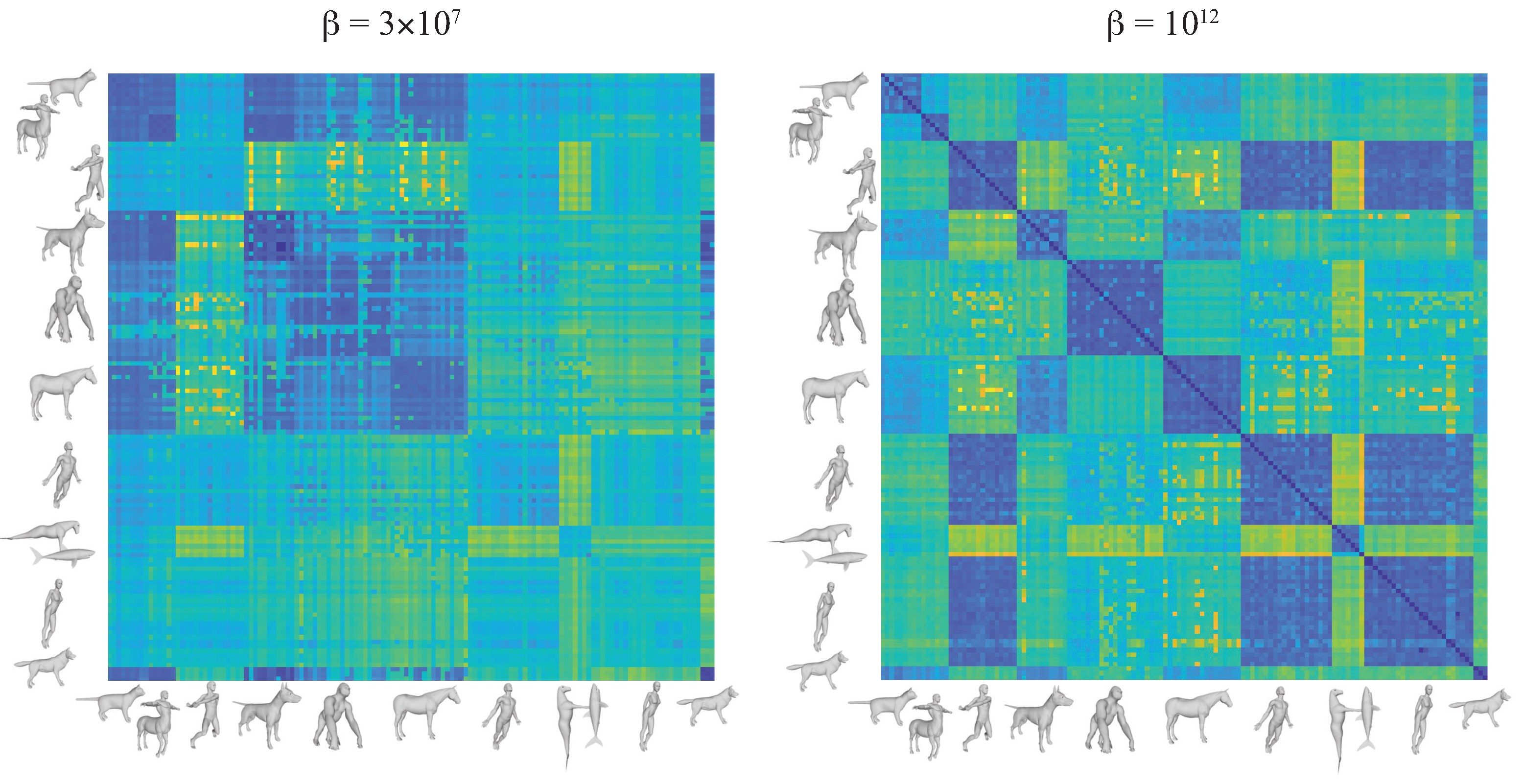
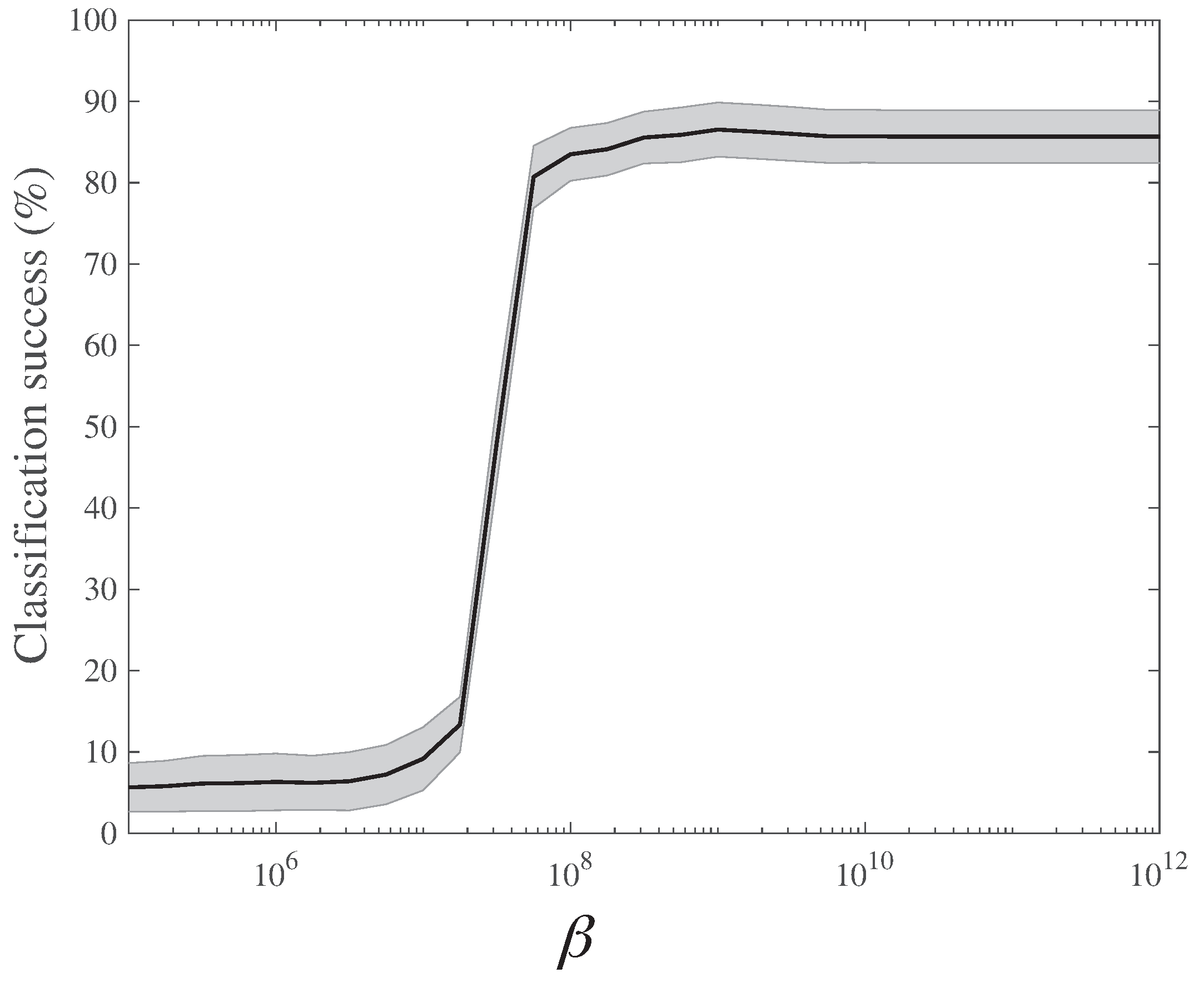
5.1. Shape Similarity: Synthetic Data from TOSCA

We use the Gromov-Wasserstein formalism to detect non-rigid shape similarity. The experiments were performed on meshes taken from the TOSCA non-rigid dataset [36,37]. Eleven classes of objects were considered (see Figure 1): 8 classes of animals, cats (9 poses), dogs (11 poses), gorilla (21 poses), horses (17 poses), seahorses (6 poses), shark (1 pose), wolves (3 poses), two male shapes, Michael (20 poses) and David (15 poses), one female shape, Victoria (24 poses), and one mythical shape, centaurs (6 poses), for a total of 133 shapes. Note that compared to the full TOSCA non rigid dataset, we removed all lions as their meshes had severe topological issues at the level of the mane. Each class consists of the same shape under different poses. These poses are the results of transformations that were designed to mimic non-rigid motions within objects (see [36,37], for details). Note that the different representatives within a class may be represented with different meshes (i.e., in addition to having different geometry those meshes may have different topologies), and may have different genera. Each shape is represented with a triangulated mesh with approximately 3400 vertices and 6600 faces, with the exception of the gorilla and seahorse meshes that include approximately 2100 vertices and 4200 faces. The Euclidean farthest point sampling procedure was used to select 1000 points from each shape’s set of vertices. In brief, one begins by selecting a point at random from the set of vertices. The second point is chosen among the remaining vertices as the one that is at the greatest distance from this first point. Subsequent points are always chosen to maximize the shortest distance to the previous points.
In each experiment, a pair of shapes i and j is represented with their sets of sampled vertices, S i and S j , and the geodesic distance matrices between those vertices, d i and d j . The geodesic distances are computed using the method proposed by Mitchell et al. [38] and implemented in the code “geodesic” by Danil Kirsanov, available at https://code.google.com/archive/p/geodesic/, and accessed on 1 June 2020. The masses associated to the vertices are set uniform, equal to 1 / N v , where Nv is the number of vertices. The GW problem is solved using FreeGW up to convergence. At each value of β , U β M F (see above), defines D M β ( i , j ) , i.e., the ( i , j ) -th element of the distance matrix D M β over all shapes in our TOSCA dataset. Note that U β M F satisfies the properties of a metric distance only when β is large (at convergence with respect to β ). We generated a set of distance matrices D M β for β ranging from 10 5 to 10 12 . Figure 1 provides graphical representations of D M β for two different temperatures, β = 3 × 10 7 and β = 10 12 . Note that the discrimination between the different shapes of TOSCA improves as β increases.
In order to assess quantitatively how well the different distance matrices D M β classify correctly the shapes in TOSCA, we designed the following set of classification experiments. We first built a reference set: we selected randomly half the shapes from each of the 11 classes within TOSCA to form this reference set. Each remaining shape was then classified by considering its distances (derived from D M β ) to all shapes in the reference set, and assigning it to the class of the shape with the shortest such distance (this is a 1-nearest neighbor classification experiment). By comparing this predicted class with the actual class to which the shape belongs we derived an estimate for the probability of correct classification P ( β ) based on D M β . We repeated this procedure over 10,000 random selections of the reference set. In Figure 2, we plot the averaged P ( β ) computed over those 10,000 experiments as a function of the inverse temperature β . The lower the temperature (or equivalently the higher the parameter β ), the more discriminative the energy U β M F is. The highest level of correct classification is already observed for β = 10 8 , i.e., significantly before convergence to the G W 2 distance, which is usually reached for β > 10 11 .

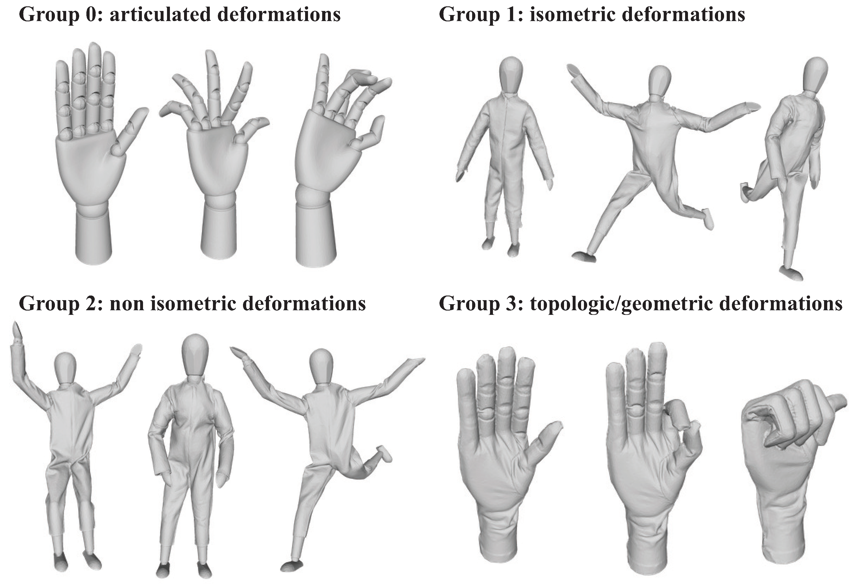
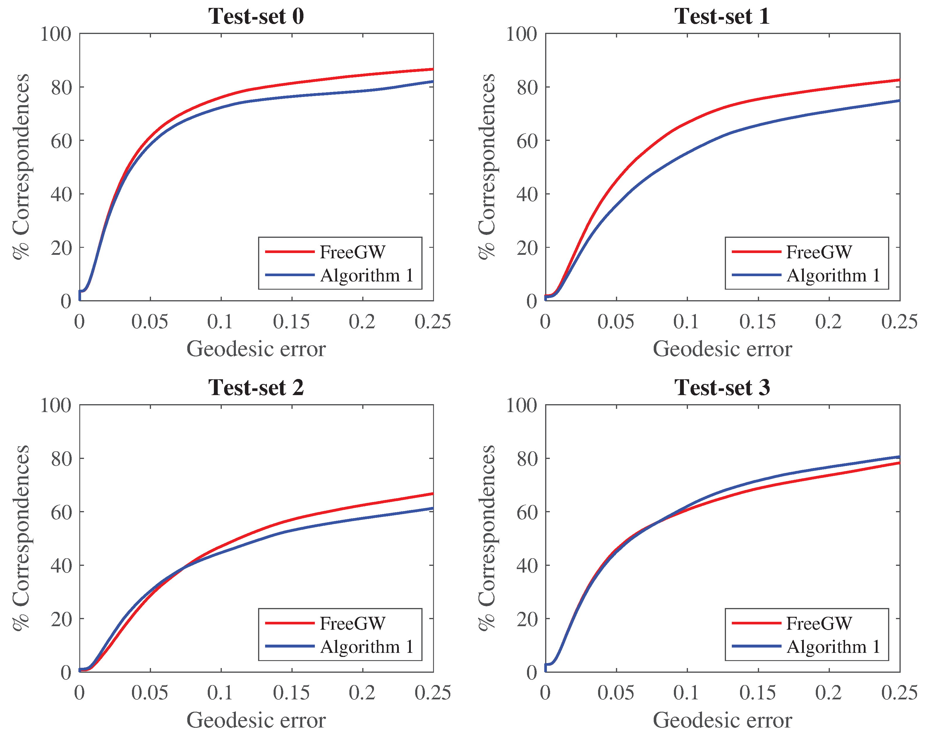
5.2. Shape Correspondence: Synthetic Data from SHREC19

The second test case we consider is shape correspondence: identifying corresponding points between two (or more) 3D shapes. Note that this is different from shape registration, namely finding a transformation that brings one shape “close” to another. Indeed, correspondence can be derived from registration, while the reverse may not be true. The Gromov-Wassertein framework allows for finding correspondence, as the latter is embedded in the optimal transport plan it computes.
To assess how well GW can recover correspondence, we considered the SHREC19 benchmark [39]. This benchmark includes 3D shapes represented with a triangular mesh of their surfaces. These shapes are derived from 3D scans of real-world objects, with each object being present in multiple poses associated with one or more types of deformation. The deformations are classified into four different groups, referred to as test-sets. Those four groups correspond to articulated deformations (group 0), isometric deformations (group 1), non-isometric deformations (group 2), and topologic/geometric deformations (group 3). Example of shapes for each test-set are provided in Figure 3.
The SHREC19 benchmark includes 76 shape pairs that are selected from the four different groups, and regrouped in four test sets (Table 1). Test-set 0 includes 14 pairs of articulating wooden hands from group 0. Test-set 1 includes 26 pairs of models corresponding to clothed humans as well as hands from group 1. Test-set 2 includes 19 pairs of models from the group 2. Each of those pairs includes a thin clothed mannequin and a larger mannequin, ensuring the the transformation is non-isometric. Finally test-set 3 includes 17 pairs of shapes from group 3 that contain challenging geometric and topological changes. We chose the low resolution version of this benchmark. In this version, each shape is represented by approximately 10,000 vertices and 20,000 triangles. For each pair of shapes, the ground-truth correspondence is known.
The quality of shape correspondence is evaluated by measuring normalized geodesics between the ground-truth (available as part of the SHREC19 dataset) and the predicted correspondence that is derived from the GW optimal coupling. Specifically, let x i be a point on shape X, y i its predicted correspondence on shape Y and g i the ground truth position of x i on Y. Note that y i and g i are both on the surface of Y. The normalized geodesic error ϵ ( x i ) between the y i and g i is computed as:
ϵ ( x i ) = d Y ( y i , g i ) a r e a ( Y ) 1 / 2 ,
where d Y ( y i , g i ) is the geodesic distance between y i and g i on the surface of Y. The geodesic distance is computed with the algorithm from Mitchell et al. [38], as described in the previous subsection.
We compared two different implementations of the GW framework, based on two different algorithms, named the fixed point method described in Algorithm 1 and the physics-based algorithm described in Algorithm 2, both implemented in FreeGW. Algorithm 1 uses a fixed regularization parameter, ϵ . To make sure that the corresponding transport plan is close to the actual GW transport plan, we chose ϵ = 10 12 . Traditional regularized OT solver do not work well for such a small ϵ . We chose therefore our own OT solver [23,24] to solve step 2 in Algorithm 1. In contrast, Algorithm 2 is based on an annealing plan with respect to the parameter β , such that when β is large, the outputs of the program are guaranteed to match the actual GW results.
In each experiment, a pair of shapes i and j is represented with their complete sets of vertices, S i and S j , and the geodesic distance matrices between those vertices, d i and d j . The masses of the vertices are set uniform. The GW problem is solved using the two algorithms mentioned above. Both derive a transport plan G. For each vertex x on i, its correspondence y on j is set to the index of the maximum value on the row corresponding to x in G. Figure 4 shows the corresponding cumulative geodesic errors for the two algorithms for the four test sets in SHREC19. We observed that Algorithm 2 as implemented in FreeGW performs better for shape correspondence than the simpler Algorithm 1, on all test sets, and significantly better from shapes with isometric deformations (test set 1).
The SHREC19 dataset was originally used as a benchmark for a competition on comparing 3D shape registration that was part of the Workshop on 3D Object Retrieval that was held in Genova, Italy in may 2019. Several groups entered in this competition; results were published in Ref. [39]. Here we compare results based on the GW framework, as presented above, with results from the five top methods that were part of this competition. We briefly describe those five methods below.
In the first method, dubbed RTPS, the correspondence map between the template shape and the target shape is computed iteratively. Each iteration is built from two successive steps. In the first step, the vertices estimated to be in correspondence between the template and target shapes are derived from the registration result obtained from the previous iteration. These computed correspondences are used to derive a correspondence mapping. In the second step, the mapping is updated by using the closest points between template and target shapes identified by the mapping to find additional points that are in correspondence [40]. The second method, NRPA, is also based on registration. It consists of four key components, namely modeling of the deformation (assumed to be anisotropic and non-isometric), computing the correspondences, pruning those correspondences, and optimizing the deformation [41]. The third method, KM, is a kernel-based method, where the registration problem is formulated as matching between a set of pairwise and pointwise descriptors, imposing a continuity prior on the mapping [42]. The fourth method, GISC, uses a genetic algorithm to find the permutation matrix that encodes the correspondences between the vertices of the two shapes to compare [43]. Note that this is the most similar method to the GW formalism, as this permutation matrix is akin to a transport plan. Finally the fifth method, WRAP, is based on the commercial software WARP that includes a wrapping tool that non-rigidly fits one 3D shape to another, from which correspondence can be derived.
We report the results of the comparisons of the qualities of the different methods in Table 1 as the areas under the curve (AUC) for the cumulative distribution functions of the geodesic normalized errors. Results are divided according to the test sets of SHREC19, as well as summarized over all test sets.
There are a few observations we can make based on Table 1. First, the AUC values provides a quantification of the quality of a method for finding correspondence: the larger the value, the better the method. In particular, Table 1 confirms that the correspondences computed from the GW framework with temperature annealing (Algorithm 2) are better than those computed with the fixed point method described in Algorithm 1. Second the four methods based on registration, RTPS, NRP, WRAP, and KM, all perform better than the method that only compute correspondences. This is likely due to the fact the the deformations included in the SHREC19 dataset are all based on a mathematical morphing, and therefore are expected to be captured with a mapping function. Finally, the GW formalism performs better than a genetic algorithm (implemented in GISC). This genetic algorithm is the one closest to the GW formalism in its concept.

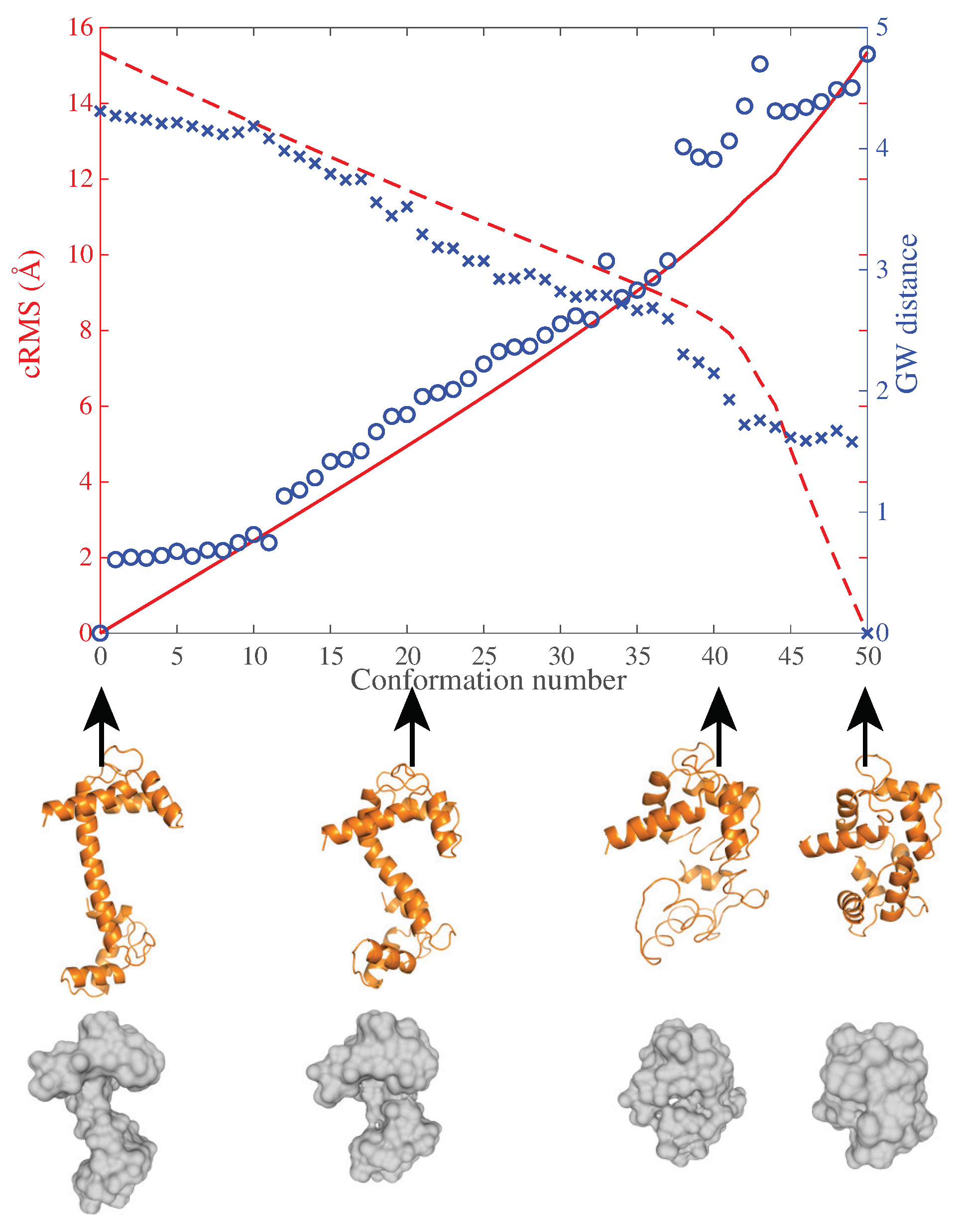
5.3. Shape Similarity: Morphodynamics of Protein Structure Surfaces

Different experimental techniques lead to different representations of protein structures. For example, high-resolution X-ray crystallography and NMR techniques derive models of proteins that include all their atoms and that are accurate at the Angstrom level. Recent progress on cryo electron microscopy (EM) can now often also reach atomic resolution. However, the difficulty of maintaining the integrity of stable complexes of interest on the various types of grids necessary to mount the sample in thin ice makes it often desirable to resort to negative staining techniques, in which case the resolution is much lower (typically 10–25 Angstroms). A low-resolution model derived from EM techniques is often represented as a density map, namely a shape characterized by its surface. Such a model is often available long before its high-resolution counterpart, as EM techniques are usually easier, faster, and cheaper to implement. It is therefore of interest to develop methods that can analyze the geometry of a protein directly from its EM density map. Such methods should generate information similar to those derived from methods that work directly on the high-resolution model of the protein structure. We consider here the problem of comparing the geometry of two protein structures using the GW distance between the surfaces of their density maps. To assess if this distance obtained from low resolution models of the protein structures mimic what could be found from high-resolution models, we compared it with the cRMS distance between atomistic models of the same proteins. We performed these tests on the protein calmodulin. Results are shown in Figure 5.
Calmodulin is a calcium binding protein that is found in all eukaryotic cells. Its structure looks like a dumbbell, with two small domains separated by a linker region. It is the flexibility of this linker that defines the ability of calmodulin to bind to a wide range of ligands [45].
We considered two conformations for calmodulin, a conformation in the absence of a ligand (referred to as the apo or ligand-free conformation) and a conformation in the presence of a substrate (referred to as holo ligand-bound conformation, where we use interchangeably the terms ligand and substrate to indicate a molecule that binds to calmodulin). Those conformations were found in the database of protein structure, the PDB [46], with codes 1CLL and 1A29, respectively. We built a trajectory between these two conformations. This trajectory is designed to mimic the structural transition that results from the binding of the ligand. We used the program MinActionPath who is designed to generate the most probable trajectory between the two conformers, namely the one with minimal action (for details, see [44]). The trajectory was sampled over 51 conformations, each represented with all the atoms of calmodulin. We then computed the distances between any two of these conformations in two different ways. First, we used the coordinate Root Mean Square (cRMS) distance computed over the C α atoms of the high-resolution structures (see Refs. [47,48] for details on how to compute the cRMS). Second, we compared the same structures using their skin surfaces [49]. To derive those skin surfaces, we started with the common convention in chemistry to represent a structure as a union of balls, with each ball corresponding to an atom. The coordinates of an atom define the center of a ball that is associated with it. The atom is also characterized with a van der Waals radius based on its chemical nature. The radius of the ball is then set to this vdW radius, plus a probe radius of R = 1.4 Å, designed to mimic a water molecule in its proximity. The skin surface is then defined as the boundary of this union of balls. We generated a triangular mesh on the skin surface using the program smesh [50,51]. We found that those meshes have similar sizes for all 51 conformations we considered, with on average approximately 40,000 vertices and 70,000 triangles. 1000 points were selected from each mesh using the Euclidean farthest point sampling procedure described above for the TOSCA dataset. We compared these sampled meshes using FreeGW.
We compared all 51 conformations of calmodulin with both the apo and holo forms, using the cRMS and the GW distances. Results of these calculations are shown in Figure 5. We do observe that the GW distances measured based on the low resolution skin surfaces correlate well with the cRMS distances computed from the high resolution, atomistic representations of the proteins. The correlation have coefficients above 0.96.

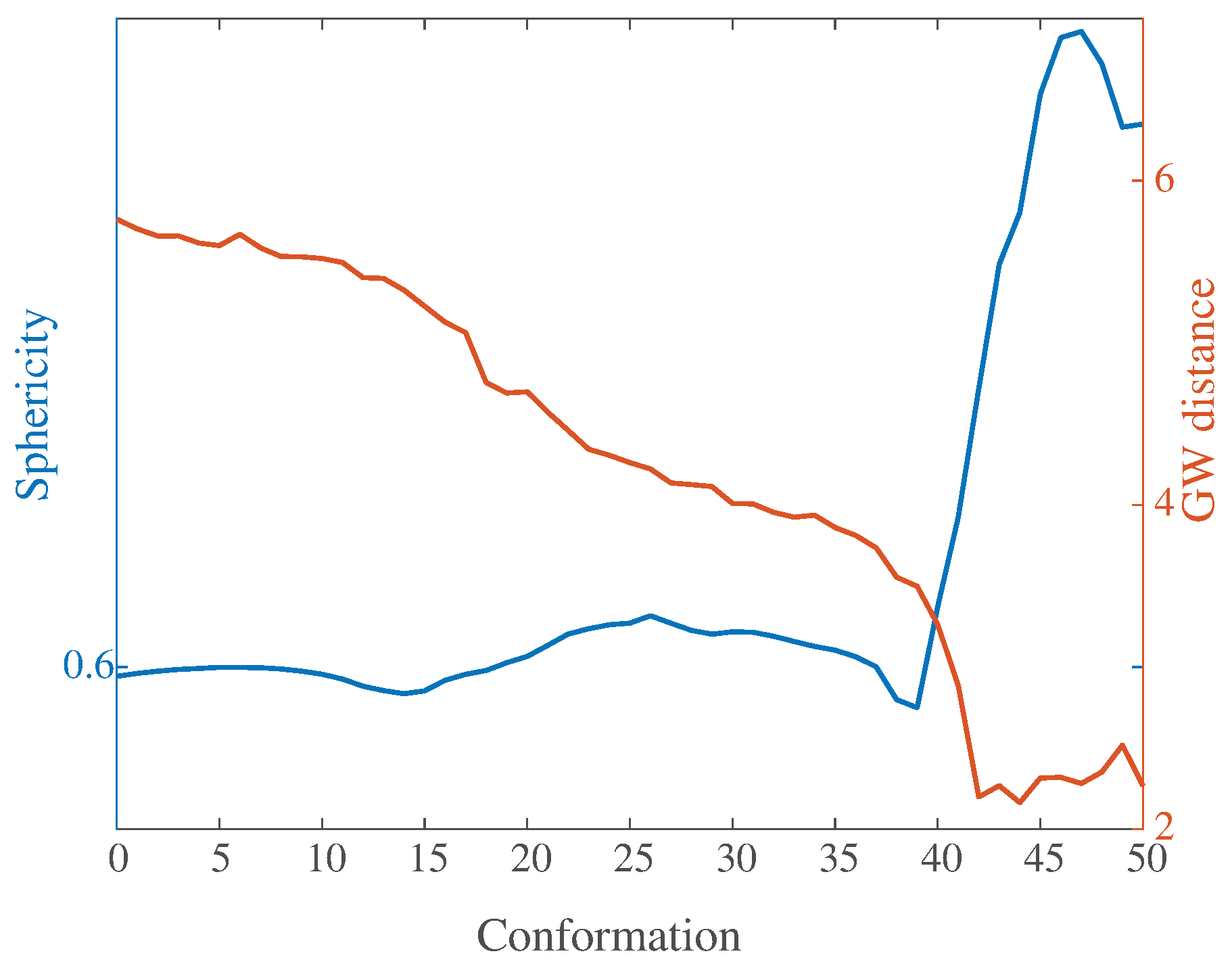
5.4. How Round Is Calmodulin?

A visual inspection of Figure 5 indicates that the ligand-bound conformation of calmodulin is more compact that its ligand-free conformation. To quantify this idea of “compactness” we use two independent measures of the surface of the proteins:
(i)
The sphericity S of a surface F quantifies how well it encloses volume. It is expressed as the surface area of an equivalent sphere (i.e., with the same volume V as the volume enclosed by F) divided by the surface area A of F:
S = π 1 / 3 ( 6 V ) 2 / 3 / A .
The sphericity is at most one, and equals one only for the round sphere,
(ii)
The GW distance between the surface of the protein and the surface of a round sphere.
We computed these two measures on all 51 conformations of the trajectory described in the previous subsection. Note that to compare the surfaces of the different conformations of calmodulin to the round sphere, we need a triangular mesh on the surface of that sphere. We generated this mesh by placing N = 1000 points uniformly on the sphere and generating a triangulation from these points. We used the Matlab package “Uniform sampling of the sphere” available from [52] to position the points and QHull [53] to generate the triangulation.
We compared the 51 sampled meshes representing the 51 conformations of calmodulin (see above for details) with the mesh representing the surface of the sphere using FreeGW. Results of these calculations are compared to the corresponding sphericity of the meshes computed using Equation (31) in Figure 6. The GW distances and the sphericity are (anti) correlated (correlation coefficient: −0.8): as the sphericity increases, the level of correspondence between the protein surface and the sphere increases, and the GW distance decreases. We observe an inflection point for the sphericity along the trajectory at the 40th conformation: the GW distance shows a similar inflection point at the same conformation. This indicates that the GW distance between a protein represented with its surface and the sphere has value as a tool to assess the compactness of that protein.

6. Discussion

In the discrete Gromov Wasserstein problem, each set of points considered is characterized by a distance matrix that captures all pairwise distances between the points. When comparing two such sets of points, there is no guarantee that those distances have the same scale. For example, for the problem of comparing 3D shapes discussed in this paper, it is possible that those shapes were captured with different 3D scanners with different internal references. The shapes themselves may have different scales, for example when comparing animals of different sizes. One approach to circumvent this problem is to normalize the corresponding distance matrices, for example by setting the largest distance in each matrix to be 1. This approach is not optimal, especially in the presence of noise, as it is biased towards a single distance. While there are other ways to normalize a distance matrix, we have used a different approach to handle the scaling problem. Instead of arbitrarily scaling the distance matrices, we have added a free scaling parameter in our approach that is concurrently optimized with the transport plan between the two sets of points.
One of the current limitation of the algorithm we propose, Algorithm 2 implemented in FreeGW, is that it is demanding in computing power. It includes three nested loops: the outer loop controls the temperature annealing, the middle loop allows for an iterative update of the scaling factor, while the most inner loop is used to solve the SPA system at a given scaling factor by iterating over a cost matrix between the two sets of points. In addition, this SPA system is non linear and therefore it is also solved iteratively (see Refs. [23,24]). We have used a Newton-Raphson approach to solve this system. It should be noted that this approach requires that the Hessian of the free energy be computed (i.e., the Jacobian of the system of non linear equation). There are ways, however, to solve the system without the need to compute second derivatives (see for example Ref. [54]). We will try such alternate approaches in future work. For large problems, the overall computational cost can become large. For example, comparing two shapes of the SHREC19 benchmark, each with 10,000 points, require on average 12,500 s (i.e., approximately 3.5 h). There are several options to reduce this computing time. First, all calculations presented in this paper were run to convergence, i.e., up to an inverse temperature β = 10 + 12 . As shown in Figure 2, if the problem is to classify shapes, there is no need to go to such a large value for β . Second, the size of the problem itself can be reduced by sampling: this is the approach we used for comparing shapes in the TOSCA dataset for example. Comparing two shapes of the TOSCA dataset, each with 1000 points, require on average 70 s. However, none of those solutions are general. For instance, sampling cannot be applied if we are interested directly in the transport plan between the two sets of points, and not just in the optimized distance between the sets. We will work on the problem of optimizing the running time of our algorithm in future studies.

7. Conclusions

In this study, we developed a novel method based on statistical physics for solving the discrete Gromov Wasserstein (GW) problem. Given two sets of measured points S 1 and S 2 associated with two possibly different metric spaces, the GW problem amounts to finding a correspondence between those points, stored in a transport plan, which minimizes an energy based on comparisons of pairwise distances within each set. We build a free energy function that, at a finite temperature, reflects the GW problem’s constraints. While the extremum of this free energy cannot be computed exactly, it can be estimated using a saddle point approximation. At each temperature, the corresponding mean field solution defines an optimal coupling between the two discrete probability measures that are compared, and a distance between those measures. We proved that this distance approaches the traditional GW distance when T 0 in a monotonic way, thereby amenable to temperature annealing. We have illustrated the usefulness of our approach on the problem of comparing shapes defined by unstructured triangulations of their surfaces and revealed that it allows for accurate and automatic non-rigid registration of shapes. We have shown that the GW distances computed from low-resolution, surface-based representations of proteins correlate well with the corresponding distances computed from atomistic models for the same proteins.
It is important to realize that the method we have proposed to solve the GW problem only applies under the assumption of balance, namely to problems in which the sum of the masses on the two discrete set of points are equal. This is often too restrictive in many applications, such as those in which only a partial mapping is sought out. The unbalanced GW problem is an open problem [55], which we intend to work on.

Author Contributions

Conceptualization, P.K., M.D. and H.O.; methodology, P.K., M.D. and H.O.; software, P.K.; formal analysis, P.K., M.D. and H.O.; investigation, P.K., M.D. and H.O.; writing: original draft preparation, P.K., M.D. and H.O. All authors have read and agreed to the published version of the manuscript.

Funding

PK acknowledges support from the National Science Foundation (grant no.1760485).

Institutional Review Board Statement

Not applicable.

Informed Consent Statement

Not applicable.

Data Availability Statement

Not applicable.

Acknowledgments

The work discussed here originated from a visit by P.K. at the Institut de Physique Théorique, CEA Saclay, France, during the fall of 2019. He thanks them for their hospitality and financial support.

Conflicts of Interest

The authors declare no conflict of interest.

Appendix A. Proof of Property 1: Monotonicity of the Free Energy and Average Energy

Let us consider two sets of points S 1 and S 2 embedded in two metric spaces ( M 1 , d 1 ) and ( M 2 , d 2 ) and mass vectors m 1 and m 2 , respectively. We associate to this system a transport plan polytope G ( S 1 , S 2 ) and a scaling factor s between distances within S 1 and distances within S 2 . Recall that any matrix G in this polytope satisfies the three conditions in Equation (8). The free energy F β ( s , S 1 , S 2 ) , internal energy E β ( s , S 1 , S 2 ) , and entropy S β ( s , S 1 , S 2 ) of this system are related through the general relation F β ( s , S 1 , S 2 ) = E β ( s , S 1 , S 2 ) T S β ( s , S 1 , S 2 ) , where T is the temperature and β = 1 / ( k B T ) .
We first prove that the volume of the polytope G ( S 1 , S 2 ) is smaller than 1. Indeed, considering the constraints that define this polytope, we have
G G ( S 1 , S 2 ) d μ 12 = 0 1 k , l d G ( k , l ) k δ l G ( k , l ) m 1 ( k ) l δ k G ( k , l ) m 2 ( l ) .
As the G ( k , l ) take values between 0 and 1, and as the delta functions restrain the space of possible transport plans, we have indeed that
0 G G ( S 1 , S 2 ) d μ 12 1 .
The internal energy is the thermodynamic average of the energy U p ( s , G ) (see Equation (10)) and is given by
E β ( s , S 1 , S 2 ) = < U ( s , G ) > s R , G G ( S 1 , S 2 ) = d β F β ( s , S 1 , S 2 ) d β ,
while the entropy is given by
S β ( s , S 1 , S 2 ) = β 2 d F β ( s , S 1 , S 2 ) d β = d F β ( s , S 1 , S 2 ) d T .
An important implication of these relations is that
d E β ( s , S 1 , S 2 ) d β = U p ( s , G ) 2 U p ( s , G ) 2 ,
where the thermodynamics averages < > are computed over R for s and over the polytope G ( S 1 , S 2 ) for G. The quantity on the right is minus the variance of the energy. It is therefore negative and this is true for all values of β . This property is true for all s and therefore for s = s ¯ , the optimal value of s. Therefore,
d E β ( S 1 , S 2 ) d β = d E β ( s ¯ , S 1 , S 2 ) d β 0 .
As a result, the internal energy of the system decreases as β increases. As U p ( s ¯ , G ) is positive, E β ( S 1 , S 2 ) is positive: it has a limit when β . This limit is the traditional GW quantity d p ( S 1 , S 2 ) (see Section 2).
The entropy is negative. Indeed, as the total number of states at an energy U p ( s , G ) is given by,
N ( U p ( s , G ) ) = G G ( S i , S j ) δ U p ( s , G ) k , l k , l G ( k , l ) d 1 ( k , k ) s · d 2 ( l , l ) p G ( k , l ) d μ 12 .
As the volume of the polytope G ( S 1 , S 2 ) is smaller than 1 (see above),
0 G G ( S i , S j ) δ U p ( s , G ) k , l k , l G ( k , l ) d 1 ( k , k ) s · d 2 ( l , l ) p G ( k , l ) d μ 12 1 ,
which implies that
N ( U p ( s , G ) ) 1 .
Since N ( U p ( s , G ) ) = e S β ( U p ( s , G ) ) , and all the properties above are valid for all s, they are valid in particular for the value s = s ¯ which minimizes the free energy. Taking s = s ¯ , we get S β ( S 1 , S 2 ) 0 for all β (or equivalently for all T). The free energy is related to the entropy by
d F β ( S 1 , S 2 ) d T = β 2 d F β ( S 1 , S 2 ) d β = S β ( S 1 , S 2 ) .
Consequently,
d F β ( S 1 , S 2 ) d β = S β ( S 1 , S 2 ) β 2 0 .
Therefore the free energy of the system decreases as β increases. Its limit for β is the same as the limit of E β , namely the GW quantity d p ( S 1 , S 2 ) , with the GW distance being d p ( S 1 , S 2 ) 1 p .

Appendix B. Proof of Proposition 2: Retrieving the Transport Plan from the SPA Solutions

Let us first recall the definition of the partition function (Equation (22))
Z β ( s , S 1 , S 2 ) = 0 1 k , l d G ( k , l ) + k , l d C ( k , l ) e β k , l k , l G ( k , l ) d 1 ( k , k ) s · d 2 ( l , l ) p G ( k , l ) × k δ l G ( k , l ) m 1 ( k ) l δ k G ( k , l ) m 2 ( l ) k , l δ k , l d 1 ( k , k ) s · d 2 ( l , l ) p G ( k , l ) C ( k , l ) .
and of the corresponding effective free energy (Equation (24))
F β = k , l D ( k , l ) C ( k , l ) k λ ( k ) m 1 ( k ) + l μ l m 2 ( l ) + k , k l , l D ( k , l ) d 1 ( k , k ) s · d 2 ( l , l ) p D ( k , l ) 1 β k , l ln 1 e β ( C ( k , l ) + λ ( k ) + μ ( l ) ) β ( C ( k , l ) + λ ( k ) + μ ( l ) ) .
F β is a function of 2 N 1 N 2 + N 1 + N 2 + 1 variables, namely D ( k , l ) and C ( k , l ) for ( k , l ) [ 1 , N 1 ] × [ 1 , N 2 ] , λ ( k ) for k [ 1 , N 1 ] , μ ( l ) for l [ 1 , N 2 ] , and s. The values of these variables that solve the SPA conditions and minimize F β with respect to s are referred to as D M F ( k , l ) , C M F ( k , l ) , λ M F ( k ) , μ M F ( l )  and s ¯ , respectively.
To find the expected values G ¯ ( k , l ) we need to introduce a vector field u and modify the partition function:
Z β ( u ) = 0 1 k , l d G ( k , l ) + k , l d C ( k , l ) e β k , l k , l G ( k , l ) d 1 ( k , k ) s · d 2 ( l , l ) p G ( k , l ) × e β ( k , l G ( k , l ) u ( k , l ) ) × k δ l G ( k , l ) m 1 ( k ) l δ k G ( k , l ) m 2 ( l ) k , l δ k , l d 1 ( k , k ) s · d 2 ( l , l ) p G ( k , l ) C ( k , l ) .
Following the same procedure as described in the main text for evaluating this modified partition function, we find,
F β ( u ) = k , l D ( k , l ) C ( k , l ) k λ ( k ) m 1 ( k ) + l μ l m 2 ( l ) + k , k l , l D ( k , l ) d 1 ( k , k ) s · d 2 ( l , l ) p D ( k , l ) 1 β k , l ln 1 e β ( C ( k , l ) + λ ( k ) + μ ( l ) u ( k , l ) ) β ( C ( k , l ) + λ ( k ) + μ ( l ) u ( k , l ) ) .
Then, the expected transport G ¯ ( k , l ) between point k in S 1 and point l in S 2  is given by
G ¯ ( k , l ) = F β ( u , v ) u ( k , l ) | u = 0 , v = 0 , C = C M F , D = D M F λ = λ M F , μ = μ M F , s = s ¯ ,
i.e.,
G ¯ ( k , l ) = e β ( C M F ( k , l ) + λ M F ( k ) + μ M F ( l ) ) e β ( C M F ( k , l ) + λ M F ( k ) + μ M F ( l ) ) 1 + 1 β ( C M F ( k , l ) + λ M F ( k ) + μ M F ( l ) ) = ϕ ( β ( C M F ( k , l ) + λ M F ( k ) + μ M F ( l ) ) ) = D M F ( k , l ) .

Appendix C. Proof of Proposition 3: Monotonicity and Limits of F MF (β) and U MF (β)

In Appendix A we have established that the exact free energy and internal energy defined in Equations (13) and 14, respectively, are monotonic functions of the parameter β , and converge to d p ( S 1 , S 2 ) when β . Here we consider the approximation of those quantities obtained with the saddle point approximation, namely the mean field values F M F and U M F , and show that they satisfy the same properties.

Appendix C.1. Monotonicity of the Free Energy

The effective free energy F β defined in Equation (23) is a function of the distance matrices d 1 and d 2 and of the real unconstrained variables C ( k , l ) , D ( k , l ) , λ ( k ) , μ ( l ) , and s. For sake of simplicity, for any ( k , l ) [ 1 , N 1 ] × [ 1 , N 2 ] , we define:
x ( k , l ) = C ( k , l ) + λ ( k ) + μ ( l ) .
The effective free energy is then
F β = k , l D ( k , l ) C ( k , l ) k λ ( k ) m 1 ( k ) + l μ l m 2 ( l ) + k , k l , l D ( k , l ) d 1 ( k , k ) s · d 2 ( l , l ) p D ( k , l ) 1 β k , l ln 1 e β x ( k , l ) β x ( k , l ) .
As written above, F β is a function of the variables β , C ( k , l ) , D ( k , l ) , λ ( k ) , μ ( l ) , and s. However, under the saddle point approximation, with s = s ¯ , namely its optimal value, the free energy takes the value F β M F , with the following constraints,
F β M F C ( k , l ) = 0 , F β M F D ( k , l ) = 0 , F β M F λ ( k ) = 0 , F β M F μ ( l ) = 0 , F β M F s = 0 ,
for all k [ 1 , N 1 ] and all l [ 1 , N 2 ] . In the following, we will use the notations d F β M F d β and F β M F β to differentiate between the total derivative and partial derivative of F β M F with respect to β , respectively. Based on the chain rule,
d F β M F d β = F β M F β + k , l F β M F C ( k , l ) C ( k , l ) β + k , l F β M F D ( k , l ) D ( k , l ) β + k F β M F λ ( k ) λ ( k ) β + l F β M F μ ( l ) μ ( l ) β + F β M F s s β .
Using the constraints defined in Equation (A14), we find that
d F β M F d β = F β M F β ,
namely that the total derivative with respect to β is in this specific case equal to the corresponding partial derivative, which is easily computed to be
d F β M F d β = 1 β 2 k , l ln 1 e β x M F ( k , l ) β x M F ( k , l ) + β x M F ( k , l ) ϕ ( β x M F ( k , l ) ) ,
where ϕ ( x ) = e x e x 1 + 1 x , as defined in Equation (26). Let f ( x ) = ln 1 e x x + x ϕ ( x ) . As mentioned in the main text of the paper, ϕ ( x ) is monotonically constrained in the interval [ 0 , 1 ] and therefore correctly represent the possible values for the corresponding transport plan. The function f ( x ) is continuous and defined over all real values x (with the extension f ( 0 ) = 0 ) and is bounded above by 0, i.e., f ( x ) 0 x R . As
d F β M F d β = 1 β 2 k , l f ( β x M F ( k , l ) ) ,
we conclude that
d F β M F d β 0 ,
namely that F β M F is a monotonically decreasing function of β . In addition, we note that F β M F is the mean field approximation of the true free energy F β and that this approximation becomes exact when β tends to . Therefore,
lim β F β M F = lim β F ( β ) = d p ( S 1 , S 2 ) ,
where d p ( S 1 , S 2 ) = ( G W p ( S 1 , S 2 ) ) p where G W p ( S 1 , S 2 ) is the traditional GW distance between the two sets of points S 1 and S 2 under the metric d 1 and d 2 , respectively.

Appendix C.2. Monotonicity of the Energy

Let G β be the transport plan at the temperature β , and let
U β = k , l k , l G β ( k , l ) d 1 ( k , k ) s · d 2 ( l , l ) p G β ( k , l ) ,
and the corresponding meanfield approximation of the internal energy at the saddle point and minimum of s = s ¯ ,
U β M F = k , l k , l G β M F ( k , l ) d 1 ( k , k ) s ¯ · d 2 ( l , l ) p G β M F ( k , l ) .
At the saddle point, we have:
l G β M F ( k , l ) = m 1 ( k ) , k G β M F ( k , l ) = m 2 ( l ) , G β M F ( k , l ) = D M F ( k , l ) = ϕ ( β x M F ( k , l ) ) ,
where ϕ and x are defined above.
Before computing d U M F ( β ) d β , let us first notice that by replacing Equation (A13) into Equation (A18), and using the constraints above, we get:
β d F M F ( β ) d β = F M F ( β ) k , l D M F ( k , l ) C M F ( k , l ) k λ M F ( k ) m 1 ( k ) l μ M F ( l ) m 2 ( l ) + k , l k , l G β M F ( k , l ) d 1 ( k , k ) s ¯ · d 2 ( l , l ) p G β M F ( k , l ) + k , l x M F ( k , l ) ϕ ( β x M F ( k , l ) ) = F M F ( β ) k , l G β M F ( k , l ) C M F ( k , l ) k , l λ M F ( k ) G β M F ( k , l ) k , l μ M F ( l ) G β M F ( k , l ) + U β M F + k , l x M F ( k , l ) G β M F ( k , l ) .
Using the definition of U β M F (Equation (A22)) and of x M F ( k , l ) (see Equation (A12)), we get
β d F β M F d β = F β M F + U β M F .
Note that this equation can be rewritten as,
U β M F = F β M F + β d F β M F d β = d ( β F β M F ) d β ,
i.e., it extends the relationship shown in Equation (A3) known between the true free energy and the average energy to their mean field counterparts.
Based on the chain rule,
d U β M F d β = U β M F β + k , l U β M F C ( k , l ) C ( k , l ) β + k , l U β M F D ( k , l ) D ( k , l ) β + k U β M F λ ( k ) λ ( k ) β + l U β M F μ ( l ) μ ( l ) β + U β M F s s β .
We compute the different partial derivatives of U β M F in this equation based on Equation (A26). For example,
U β M F C ( k , l ) = F β M F C ( k , l ) + β C ( k , l ) F β M F β = F β M F C ( k , l ) + β β F β M F C ( k , l ) = 0 ,
where the zero is a consequence of the SPA constraints. Similarly, we can show that
U β M F D ( k , l ) = U β M F λ ( k ) = U β M F μ ( l ) = U β M F s = 0 .
Replacing in Equation (A27) and using Equation (A26) we get
d U β M F d β = U β M F β = 2 F β M F β + β β F β M F β = 2 F β M F β + β 2 β F β M F β + 1 β 2 k , l β x M F ( k , l ) 2 ϕ ( β x M F ( k , l ) ) = k , l β x M F ( k , l ) 2 ϕ ( β x M F ( k , l ) ) .
As x M F ( k , l ) 2 is always positive, and ϕ ( x ) is always negative, we have
d U β M F d β 0 ,
and the function U β M F is a monotonically decreasing function of β . In addition, we note that U β M F is the mean field approximation of the true internal energy E β and that this approximation becomes exact when β tends to . Therefore,
lim β U β M F = lim β E ( β ) = d p ( S 1 , S 2 ) ,
where d p ( S 1 , S 2 ) = ( G W p ( S 1 , S 2 ) ) p where G W p ( S 1 , S 2 ) is the traditional GW distance between the two sets of points S 1 and S 2 under the metric d 1 and d 2 , respectively.

References

  1. Monge, G. Mémoire sur la theorie des deblais et des remblais. Hist. l’Acad. R. Sci. Mem. Math. Phys. Tires Regist. Cette Acad. 1781, 1784, 666–704. [Google Scholar]
  2. Léonard, C. A survey of the Schrödinger problem and some of its connections with optimal transport. Discret. Contin. Dyn. Syst. Ser. A 2014, 34, 1533–1574. [Google Scholar] [CrossRef]
  3. Kantorovich, L. On the transfer of masses. Dokl. Acad. Nauk. USSR 1942, 37, 7–8. [Google Scholar]
  4. Villani, C. Optimal Transport: Old and New; Grundlehren der Mathematischen Wissenschaften; Springer: Berlin/Heidelberg, Germany, 2008. [Google Scholar]
  5. Peyré, G.; Cuturi, M. Computational Optimal Transport. arXiv 2018, arXiv:1803.00567. [Google Scholar]
  6. Villani, C. Topics in Optimal Transportation; Graduate Studies in Mathematics; American Mathematical Society: Providence, RI, USA, 2003. [Google Scholar]
  7. Mémoli, F. On the use of Gromov-Hausdorff Distances for Shape Comparison. In Proceedings of the Eurographics Symposium on Point-Based Graphics, Prague, Czech Republic, 2–3 September 2007; pp. 81–90. [Google Scholar]
  8. Mémoli, F. Gromov-Wasserstein distances and the metric approach to object matching. Found. Comput. Math. 2011, 11, 417–487. [Google Scholar] [CrossRef]
  9. Boyer, D.; Lipman, Y.; StClair, E.; Puente, J.; Patel, B.; Funkhouser, T.; Jernvall, J.; Daubechies, I. Algorithms to automatically quantify the geometric similarity of anatomical surface. Proc. Natl. Acad. Sci. USA 2011, 108, 18221–18226. [Google Scholar] [CrossRef] [PubMed] [Green Version]
  10. Alvarez-Melis, D.; Jaakkola, T.S. Gromov-Wasserstein alignment of word embedding spaces. arXiv 2018, arXiv:1809.00013. [Google Scholar]
  11. Yan, Y.; Li, W.; Wu, H.; Min, H.; Tan, M.; Wu, Q. Semi-Supervised Optimal Transport for Heterogeneous Domain Adaptation. In Proceedings of the IJCAI, Stockholm, Sweden, 13–19 July 2018; Volume 7, pp. 2969–2975. [Google Scholar]
  12. Ezuz, D.; Solomon, J.; Kim, V.G.; Ben-Chen, M. GWCNN: A metric alignment layer for deep shape analysis. In Proceedings of the Computer Graphics Forum, Lyon, France, 24–28 April; 2017; Volume 36, pp. 49–57. [Google Scholar]
  13. Nguyen, D.H.; Tsuda, K. On a linear fused Gromov-Wasserstein distance for graph structured data. Pattern Recognit. 2023, 138, 109351. [Google Scholar] [CrossRef]
  14. Titouan, V.; Courty, N.; Tavenard, R.; Flamary, R. Optimal transport for structured data with application on graphs. In Proceedings of the International Conference on Machine Learning, Long Beach, CA, USA, 9–15 June 2019; pp. 6275–6284. [Google Scholar]
  15. Zheng, L.; Xiao, Y.; Niu, L. A brief survey on Computational Gromov-Wasserstein distance. Procedia Comput. Sci. 2022, 199, 697–702. [Google Scholar] [CrossRef]
  16. Chowdhury, S.; Needham, T. Generalized spectral clustering via Gromov-Wasserstein learning. In Proceedings of the International Conference on Artificial Intelligence and Statistics, Virtual, 13–15 April 2021; pp. 712–720. [Google Scholar]
  17. Bunne, C.; Alvarez-Melis, D.; Krause, A.; Jegelka, S. Learning generative models across incomparable spaces. In Proceedings of the International Conference on Machine Learning, Long Beach, CA, USA, 9–15 June 2019; pp. 851–861. [Google Scholar]
  18. Cuturi, M. Sinkhorn Distances: Lightspeed Computation of Optimal Transport. In Advances in Neural Information Processing Systems 26; Burges, C.J.C., Bottou, L., Welling, M., Ghahramani, Z., Weinberger, K.Q., Eds.; Curran Associates, Inc.: Red Hook, NY, USA, 2013; pp. 2292–2300. [Google Scholar]
  19. Deming, W.E.; Stephan, F.F. On a least squares adjustment of a sampled frequency table when the expected marginal totals are known. Ann. Math. Stat. 1940, 11, 427–444. [Google Scholar] [CrossRef]
  20. Sinkhorn, R. A relationship between arbitrary positive matrices and doubly stochastic matrices. Ann. Math. Stat. 1964, 35, 876–879. [Google Scholar] [CrossRef]
  21. Sinkhorn, R.; Knopp, P. Concerning nonnegative matrices and doubly stochastic matrices. Pacific J. Math. 1967, 21, 343–348. [Google Scholar] [CrossRef] [Green Version]
  22. Peyré, G.; Cuturi, M.; Solomon, J. Gromov-Wasserstein Averaging of Kernel and Distance Matrices. In Proceedings of the Proceeding ICML’16, New York, NY, USA, 19–24 June 2016; pp. 2664–2672. [Google Scholar]
  23. Koehl, P.; Delarue, M.; Orland, H. A statistical physics formulation of the optimal transport problem. Phys. Rev. Lett. 2019, 123, 040603. [Google Scholar] [CrossRef] [PubMed]
  24. Koehl, P.; Delarue, M.; Orland, H. Finite temperature optimal transport. Phys. Rev. E 2019, 100, 013310. [Google Scholar] [CrossRef] [PubMed]
  25. Koehl, P.; Orland, H. Fast computation of exact solutions of generic and degenerate assignment problems. Phys. Rev. E 2021, 103, 042101. [Google Scholar] [CrossRef]
  26. Koehl, P.; Delarue, M.; Orland, H. Physics approach to the variable-mass optimal-transport problem. Phys. Rev. E 2021, 103, 012113. [Google Scholar] [CrossRef]
  27. Gould, N.I.; Toint, P.L. A quadratic programming bibliography. Numer. Anal. Group Intern. Rep. 2000, 1, 32. [Google Scholar]
  28. Wright, S. Continuous optimization (nonlinear and linear programming). In The Princeton Companion to Applied Mathematics; Higham, N., Dennis, M., Glendinning, P., Martin, P., Sentosa, F., Tanner, J., Eds.; Princeton University Press: Princeton, NJ, USA, 2015; pp. 281–293. [Google Scholar]
  29. Pardalos, P.; Vavasis, S. Quadratic programming with one negative eigenvalue is (strongly) NP-hard. J. Glob. Optim. 1991, 1, 15–22. [Google Scholar] [CrossRef]
  30. Nocedal, J.; Wright, S.J. Quadratic programming. Numer. Optim. 2006, 448–492. [Google Scholar]
  31. Benamou, J.; Carlier, G.; Cuturi, M.; Nenna, L.; Peyré, G. Iterative Bregman Projections for Regularized Transportation Problems. SIAM J. Sci. Comput. 2015, 37, A1111–A1138. [Google Scholar] [CrossRef] [Green Version]
  32. Genevay, A.; Cuturi, M.; Peyré, G.; Bach, F. Stochastic Optimization for Large-scale Optimal Transport. In Advances in Neural Information Processing Systems 29; Curran Associates, Inc.: Red Hook, NY, USA, 2016; pp. 3440–3448. [Google Scholar]
  33. Schmitzer, B. Stabilized Sparse Scaling Algorithms for Entropy Regularized Transport Problems. arXiv 2016, arXiv:1610.06519. [Google Scholar] [CrossRef] [Green Version]
  34. Dvurechensky, P.; Gasnikov, A.; Kroshnin, A. Computational Optimal Transport: Complexity by Accelerated Gradient Descent Is Better Than by Sinkhorn’s Algorithm. In Proceedings of the 35th International Conference on Machine Learning, Stockholm, Sweden, 10–15 July 2018; pp. 1367–1376. [Google Scholar]
  35. Chizat, L.; Peyré, G.; Schmitzer, B.; Vialard, F.X. Scaling Algorithms for Unbalanced Transport Problems. Math. Comp. 2018, 87, 2563–2609. [Google Scholar] [CrossRef]
  36. Bronstein, A.; Bronstein, M.; Kimmel, R. Efficient computation of isometry-invariant distances between surfaces. SIAM J. Sci. Comput. 2006, 28, 1812–1836. [Google Scholar] [CrossRef] [Green Version]
  37. Bronstein, A.; Bronstein, M.; Kimmel, R. Calculus of non-rigid surfaces for geometry and texture manipulation. IEEE Trans. Vis. Comput. Graph 2007, 13, 902–913. [Google Scholar] [CrossRef] [PubMed] [Green Version]
  38. Mitchell, J.; Mount, D.; Papadimitriou, C. The discrete geodesic problem. SIAM J. Comput. 1987, 16, 647–668. [Google Scholar] [CrossRef]
  39. Dyke, R.M.; Stride, C.; Lai, Y.K.; Rosin, P.L.; Aubry, M.; Boyarski, A.; Bronstein, A.M.; Bronstein, M.M.; Cremers, D.; Fisher, M.; et al. Shape Correspondence with Isometric and Non-Isometric Deformations. In Proceedings of the Eurographics Workshop on 3D Object Retrieval; Biasotti, S., Lavoué, G., Veltkamp, R., Eds.; The Eurographics Association: Eindhoven, The Netherlands, 2019. [Google Scholar]
  40. Li, K.; Yang, J.; Lai, Y.K.; Guo, D. Robust non-rigid registration with reweighted position and transformation sparsity. IEEE Trans. Visual. Comput. Graphics 2018, 25, 2255–2269. [Google Scholar] [CrossRef] [Green Version]
  41. Dyke, R.; Lai, Y.K.; Rosin, P.; Tam, G. Non-rigid registration under anisotropic deformations. Comput. Aided Geom. Des. 2019, 71, 142–156. [Google Scholar] [CrossRef]
  42. Vestner, M.; Lähner, Z.; Boyarski, A.; Litany, O.; Slossberg, R.; Remez, T.; Rodolà, E.; Bronstein, A.; Bronstein, M.; Kimmel, R.; et al. Efficient deformable shape correspondence via kernel matching. In Proceedings of the 2017 International Conference on 3D Vision (3DV), Qingdao, China, 10–12 October 2017; IEEE: Piscataway, NJ, USA, 2017; pp. 517–526. [Google Scholar]
  43. Sahillioğlu, Y. A genetic isometric shape correspondence algorithm with adaptive sampling. ACM Trans. Graph. (ToG) 2018, 37, 1–14. [Google Scholar] [CrossRef]
  44. Franklin, J.; Koehl, P.; Doniach, S.; Delarue, M. MinActionPath: Maximum likelihood trajectory for large-scale structural transitions in a coarse-grained locally harmonic energy landscape. Nucl. Acids. Res. 2007, 35, W477–W482. [Google Scholar] [CrossRef] [Green Version]
  45. Chou, J.; Li, S.; Klee, C.; Bax, A. Solution structure of Ca(2+)-calmodulin reveals flexible hand-like properties of its domains. Nat. Struct. Biol. 2001, 8, 990–997. [Google Scholar] [CrossRef]
  46. Berman, H.; Westbrook, J.; Feng, Z.; Gilliland, G.; Bhat, T.; Weissig, H.; Shindyalov, I.; Bourne, P. The Protein Data Bank. Nucleic Acids Res. 2000, 28, 235–242. [Google Scholar] [CrossRef] [PubMed] [Green Version]
  47. Kabsch, W. A solution for the best rotation to relate two sets of vectors. Acta Crystallogr. 1976, 32, 922–923. [Google Scholar] [CrossRef]
  48. Coutsias, E.; Seok, C.; Dill, K. Using quaternions to calculate RMSD. J. Comput. Sci. 2004, 25, 1849–1857. [Google Scholar] [CrossRef] [PubMed]
  49. Edelsbrunner, H. Deformable Smooth Surface Design. Discret. Comput. Geom. 1999, 21, 87–115. [Google Scholar] [CrossRef] [Green Version]
  50. Cheng, H.; Shi, X. Guaranteed Quality Triangulation of Molecular Skin Surfaces. In Proceedings of the IEEE Visualization, Austin, TX, USA, 10–15 October 2004; pp. 481–488. [Google Scholar]
  51. Cheng, H.; Shi, X. Quality Mesh Generation for Molecular Skin Surfaces Using Restricted Union of Balls. In Proceedings of the IEEE Visualization, Minneapolis, MN, USA, 23–28 October 2005; pp. 399–405. [Google Scholar]
  52. Semeshko, A. Suite of Functions to Perform Uniform Sampling of a Sphere. GitHub. Available online: https://github.com/AntonSemechko/S2-Sampling-Toolbox (accessed on 2 January 2023).
  53. Barber, C.B.; Dobkin, D.; Huhdanpaa, H. The Quickhull Algorithm for Convex Hulls. ACM Trans. Math. Softw. 1996, 22, 469–483. [Google Scholar] [CrossRef] [Green Version]
  54. Abdul-Hassan, N.Y.; Ali, A.H.; Park, C. A new fifth-order iterative method free from second derivative for solving nonlinear equations. J. Appl. Math. Comput. 2021, 68, 2877–2886. [Google Scholar] [CrossRef]
  55. Séjourné, T.; Peyré, G.; Vialard, F.X. Unbalanced Optimal Transport, from theory to numerics. arXiv 2022, arXiv:2211.08775. [Google Scholar]
Figure 1. Distance matrices for shape similarity within the TOSCA dataset using the Gromov-Wassertein framework at two different “temperatures”, β = 3 × 10 7 (left) and β = 10 12 (right). Blue colors represent small distances (high similarity), while yellow colors represent large distances (low similarity).
Algorithms 16 00131 g001
Figure 2. Quality of 3D shape recognition based of the temperature-dependent GW distances as a function of temperature. The probability of classifying correctly a shape into its own class within the TOSCA dataset using the distance measure D M β U β M F (see text for details) is plotted against β , the inverse of the temperature. The curve is generated from the arithmetic means over 10,000 experiments (see text for details). Shaded areas represent standard deviations over those experiments.
Algorithms 16 00131 g002
Figure 3. Examples of shapes in each group of the SHREC19 benchmark [39].
Algorithms 16 00131 g003
Figure 4. Cumulative distribution functions for the geodesic errors for the correspondence computed with FreeGW (red), which implements an annealing procedure in the regularization parameter β , and computed with Algorithm 1 (blue), that only considers one regularization value (see text for details). Results are shown for all four test sets in SHREC19, that consider articulated deformations (test set 0), isometric deformations (test set 1), non-isometric deformations (test set 2), and topological or geometric deformations (test set 3).
Algorithms 16 00131 g004
Figure 5. Analyzing the dynamics of the conformational transition of calmodulin using coarse and high resolution models of the protein. We built a trajectory including 51 conformations between the apo (i.e., ligand-free) structure and an holo (i.e., with a ligand-bound) structure of the protein calmodulin using the program MinActionPath [44]. The transition between those two conformations leads to significant changes in the structure, as illustrated with the models of the structures shown below the horizontal axis. For all those 51 conformations, we computed their cRMS distances to the apo structure (structure number 0). These cRMS values are plotted versus the conformation number as a red solid line. In parallel, we plot the GW distance between the surfaces representing the same conformers and the surface of the apo protein as blue dots. The cRMS values and corresponding GW values exhibit a high correlation (0.985). The same observation can be made when comparing the 51 conformations with the holo structure based on cRMS (dashed red line) and based on the GW distance between surfaces (blue x’s). The cartoon representations of the high resolution structures and surface representations of the same structure are shown for a few conformations along the trajectory below the horizontal axis.
Algorithms 16 00131 g005
Figure 6. The sphericity (left axis, blue) and the GW distance to the round sphere (right axis, red) of the 51 conformations of calmodulin in its trajectory from the ligand-free to the ligand-bound conformations.
Algorithms 16 00131 g006
Table 1. Quality of different methods for computing correspondence between 3D shapes.
Method a Test-Set 0Test-Set 1Test-Set 2Test-Set 3All Test Sets
RPTS [40]0.920 b0.9260.8240.9290.899
NRP [41]0.8780.8990.8010.8580.862
WRAP0.8530.9200.7720.8700.856
KM [42]0.7600.8650.7570.7990.804
FreeGW d0.7060.8790.5500.3200.588
Algo1 e0.6660.8460.4900.3380.548
GISC [43]0.5650.6590.674NA cNA c
a Rows are in descending order of score over all test sets. b Area under the curve (AUC) for the cumulative distribution functions of the normalized geodesic errors in the correspondences. Results for the first five methods are derived from Ref. [39]. c Not Available in Ref. [39]. d Our results based on Algorithm 2 that consider an annealing procedure in the regularization parameters. e Our results based on Algorithm 1.
Disclaimer/Publisher’s Note: The statements, opinions and data contained in all publications are solely those of the individual author(s) and contributor(s) and not of MDPI and/or the editor(s). MDPI and/or the editor(s) disclaim responsibility for any injury to people or property resulting from any ideas, methods, instructions or products referred to in the content.

