Article

Apollonian Packing of Circles within Ellipses

1
Department of Information Engineering, Electronics and Telecommunications, Sapienza University of Rome, Via Eudossiana 18, 00184 Rome, Italy
2
CNIT: National, Inter-University Consortium for Telecommunications, Viale G.P. Usberti, 181/A, 43124 Parma, Italy
*
Author to whom correspondence should be addressed.
Algorithms 2023, 16(3), 129; https://doi.org/10.3390/a16030129
Submission received: 16 January 2023 / Revised: 11 February 2023 / Accepted: 16 February 2023 / Published: 24 February 2023
(This article belongs to the Special Issue Computational Methods and Optimization for Numerical Analysis)

Abstract

:
The purpose of a circle packing procedure is to fill up a predefined, geometrical, closed contour with a maximum finite number of circles. The subject has received considerable attention in pure and applied sciences and has proved to be highly effective in connection with many a problem in logistics and technology. The well-known Apollonian circle packing achieves the packing of an infinite number of mutually tangent smaller circles of decreasing radii, internal or tangent to the outer boundary. Algorithms are available in the literature for the packing of equal-radius circles within an ellipse for global optimization purposes. In this paper, we propose a new algorithm for the Apollonian packing of circles within an ellipse, based on fundamental numerical methods, granting suitable speed, accuracy and stability. The novelty of the proposed approach consists in its applicability to the Apollonian packing of circles within a generic, closed, convex contour, if the parametrization of its outer boundary is given.

1. Introduction

Circle packings achieve the optimized filling of a generic finite plane region with a number of non-overlapping circles. Such topic has aroused a great interest in mathematics, physics, geophysics and operational research and has been fruitfully applied to a large variety of problems in logistics and technology [1]. A nonlinear programming-based algorithm for the packing of circles within ellipses is proposed in [2], achieving covering with a finite amount of equal-radius enclosed circles for global optimization purposes. The well-known Apollonian circle packing (or Apollonian gasket) achieves the filling of a bounded or unbounded plane region with an infinite number of mutually tangent smaller circles of decreasing radii, internal or tangent to the outer boundary, by iteratively or recursively filling the interstices left between tangent circles [3]. Such geometrical arrangement has been used in a variety of physical models, and its generalization to space-filling bearings has been applied to the understanding of geological sheer bands [4,5]. The construction of an Apollonian circle packing, granted by an ancient theorem of Apollonius of Perga, may be reduced to an elementary geometric problem, i.e., the search for a circle that is tangent to three mutually tangent circles given their three centers and radii. The first solution to this fundamental problem is ascribed to René Descartes in 1643, to  be independently rediscovered by Sir Frederick Soddy as the Kissing Circles problem in 1936 [6]. The solution may undergo a simple formulation in the complex domain [7], ready for straightforward application in a numerical algorithm. In addition to the algebraic solution of the problem by means of the Descartes theorem, a classical geometrical construction of a circle that is tangent to three other given circles by means of rule and compass is available [8], and a very elegant and mathematically revealing approach based on circle inversion mapping in the complex plane [9] is commonly used in implementations [10]. The aforementioned solution methods are not easily extensible to the case of an elliptical outer boundary. To overcome this limitation, we developed an elementary interpretation of the construction of tangent packing circles, which is based on the so-called menaechmics, i.e., the search for solutions to an algebraic or geometric problem by means of intersections of conic sections [11]. The proposed Menaechmic method, applied to the construction of Apollonian circle packings within ellipses, has proved to grant suitable speed, accuracy and stability. The novelty of the proposed approach consists in its applicability to the packing of a generic, closed, convex contour, if the parametrization of its outer boundary is given. The present work was developed within a research program on electromagnetic field scattering using elliptic, cylindrical dielectric structures, stemming from the need to simulate a dielectric cylinder of arbitrary cross-section with a finite number of circular dielectric cylinders enclosed within the assigned arbitrary contour [12,13,14,15]. For this purpose, Apollonian circle packing achieves the covering of a circular, elliptic or generically closed contour, optimizing the number of mutually tangent smaller circles and consequently reducing the computational complexity of simulations.
In Section 2 of this paper, an algorithm achieving Apollonian circle packing within an elliptic domain is described, together with its implementation in a specific code. In Section 3, results are presented and discussed. Conclusions are given in Section 4.

2. Materials and Methods

2.1. The Descartes Formula

2.1.1. The Descartes Formula

The Descartes theorem [7] applies to any configuration of four mutually tangent circles in which the interiors of all circles are disjoint; in such case, the four circles are said to be arranged in a so-called Descartes configuration.
The theorem states that any Descartes configuration of four mutually tangent circles with  curvatures k j satisfies
j = 1 4 ( k i ) 2 = 1 2 j = 1 4 k j 2 ,
where k j = 1 / r j ( j = 1 , 2 , 3 , 4 ) are the curvatures of the circles and r j are the radii of the circles.
The theorem in its complex form [6] states that any Descartes configuration of four mutually tangent circles with curvatures k j and centers z j = x j + i y j satisfies
j = 1 4 ( k i z i ) 2 = 1 2 j = 1 4 k j z j 2 .
As stated in [7], the theorem may be extended to include the case in which three of the circles are internally tangent to the fourth one by defining the concept of oriented circle with signed values of radius and curvature and by characterizing the fourth circle, which encloses the other three, with negative values of such parameters. In this approach, the theorem is applicable to any oriented Descartes configuration defined by either one of the following statements: (i) the interiors of all oriented circles are disjoint; (ii) the interiors of all oriented circles are disjoint when all orientations are reversed.
By directly solving the quadratic equations that constitute the thesis of the theorem [7], we obtain the formula expressing the curvature of the fourth circle in terms of the curvatures of the remaining circles in the Descartes configuration.
k 4 1 , 2 = k 1 + k 2 + k 3 ± 2 k 1 k 2 + k 1 k 3 + k 2 k 3 .
The two algebraic solutions, corresponding to the two options for the ± symbol, refer to the two possible solutions of the geometric problem, i.e., it is possible to construct up to two distinct circles that are tangent to three mutually tangent circles in a Descartes configuration. By means of a similar procedure, starting from Equation (2), it is possible to obtain a corresponding formula for circle center z 4 .
z 4 1 , 2 = z 1 k 1 + z 2 k 2 + z 3 k 3 ± 2 z 1 z 2 k 1 k 2 + z 1 z 3 k 1 k 3 + z 2 z 3 k 2 k 3 k 4 .
In order to achieve correct results in the implementation of the solution formulas expressed in Equations (3) and (4), attention should be paid to the multivalued character of the square root function in the complex plane. The choice of the correct complex square root value must be carefully carried out in the eventuality of the branch-cut crossing of the square root argument in Equation (4).

2.1.2. Scaffolding of the Gasket

As stated in [7], the Apollonian packing of a given circle is completely specified by any three mutually tangent circles in it; thus, it is possible to achieve a complete packing by applying iteratively or recursively Equations (3) and (4) starting from an initial Descartes configuration or a larger portion of the final packing. In the following, the initial configuration will be referred to as the scaffolding of the gasket.

2.2. Apollonian Circle Packing within an Ellipse

2.2.1. Point-to-Ellipse Distance

The proposed approach to Apollonian circle packing within an elliptic domain is based on the evaluation of the distance between a point P and an ellipse E , owing to the necessity of satisfying a circle tangency condition on the outer elliptical boundary. In [2,16], a special “distance revealing” type of parametrization is described; in addition, several algorithms for the numerical computation of the point-to-ellipse distance have been proposed and are easily available as open access contributions [17,18]. In the case under analysis, the distance must only be evaluated for points within the elliptic boundary, and the algorithm must be chosen to provide an estimation of the distance value and, at the same time, the determination of point E ¯ of the ellipse, which is at a minimum distance from P. For this reason, a solution based on golden section search or the Fibonacci search algorithm [19,20] is sufficient for our purposes, conveying high reliability and, although characterized by a linear convergence rate, being suitable to be applied to other convex figures, prior appropriate parametrization of the closed curvilinear boundary.

2.2.2. Scaffolding of the Elliptic Domain

As in the case of a circular Apollonian packing, Apollonian packing within a non-circular plane domain is completely determined by defining the outer boundary and an initial scaffolding configuration of circles. Given the outer boundary and the initial scaffolding configuration, all subsequent circles in the packing sequence determined by the algorithm are univocally defined. Thus, each new circle of the packing sequence to be found must be in a Descartes-like configuration, i.e., it must be either externally tangent to three preceding circles or externally tangent to two circles and internally tangent to the outer boundary of the plane domain. For this reason, we can define, as a scaffolding configuration for an Apollonian circle packing within a plane domain D , any configuration of circles that has the following characteristics:
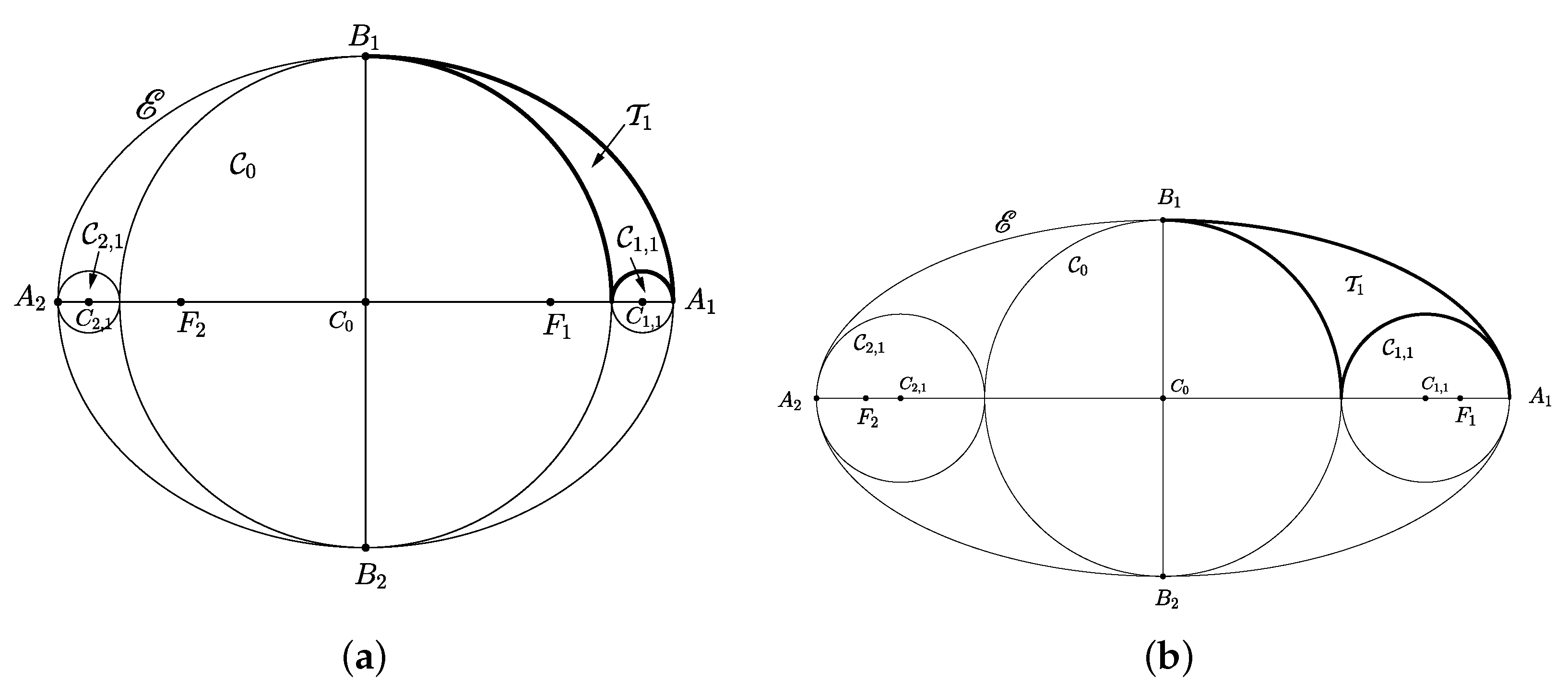
  • The scaffolding circles are internal to D .
  • The difference between domain D and the scaffolding circles must be composed by a finite number of arbelos or deltoid-like [21,22] curvilinear triangles formed by arcs of the scaffolding circles or of the outer boundary, tangent in the vertexes.
The effectiveness of the proposed algorithm is independent from the choice of the scaffolding configuration to which it is applied, even in the case of non-symmetric initial configurations; thus, the choice of the scaffolding configuration within a given ellipse is not univocal, with each configuration giving rise to a different circle packing within the same ellipse. Since the determination of the circle filling in a deltoid-like curvilinear triangle may be obtained by means of the Descartes formula, attention must be paid to the filling of the arbelos-like curvilinear triangles. For illustrative purposes, we will focus on scaffolding structures for an Apollonian circle packing within an elliptic domain ε , having major axis 2 a and minor axis 2 b ( a , b R , a b ), which are symmetric with respect to the ellipse axes and composed by the following 2 N 1 ( N N , N > 0 ) circles:
  • A larger circle C 0 , having radius r 0 = b , centered on the ellipse symmetry center.
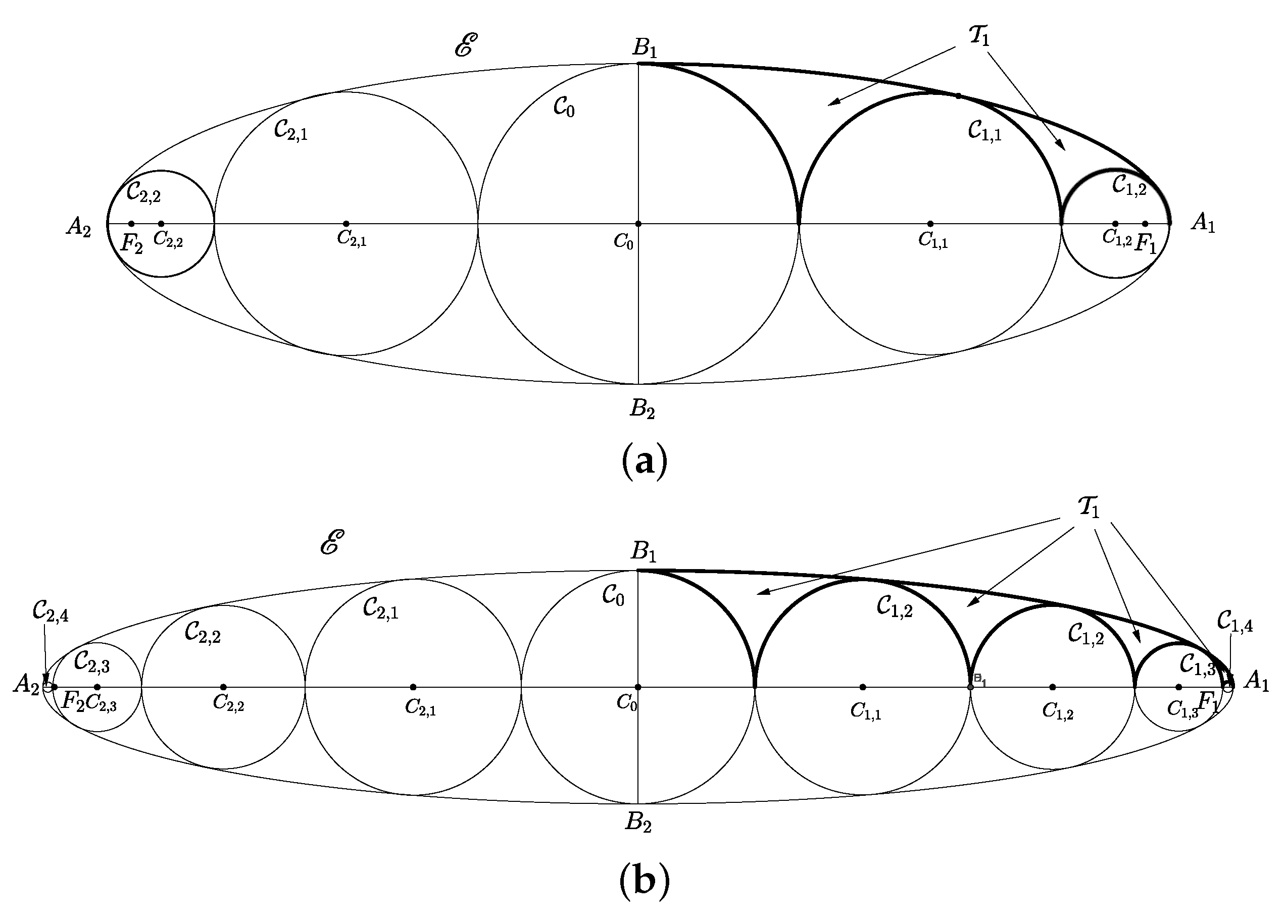
  • If N > 1 , two sequences of N 1 non-intersecting, consecutively tangent circles C i , 1 , , C i , N 1 ( i = 1 , 2 ; N N , N 1 ), tangent to boundary ellipse E , whose centers C i , n are external to C 0 and are placed on the major axis of the ellipse, with each one of circles C i , 1 being externally tangent to C 0 .
Two examples of typical scaffolding layouts for N = 2 , 3 , 5 in the cases of a / b = 5 / 4 , a / b = 2 and a / b = 5 are shown in Figure 1 and Figure 2.
By exploiting the symmetry properties of the scaffolding, it is possible to achieve the complete packing of elliptic domain ε by filling plane region T 1 inside curvilinear triangle A 1 B 1 C 0 and outside scaffolding circles C 1 , n , as shown in Figure 1 and Figure 2, and by generating 4 replicas of the T 1 packing by symmetry with respect to the ellipse axes.

2.2.3. Scaffolding Circle Algorithm
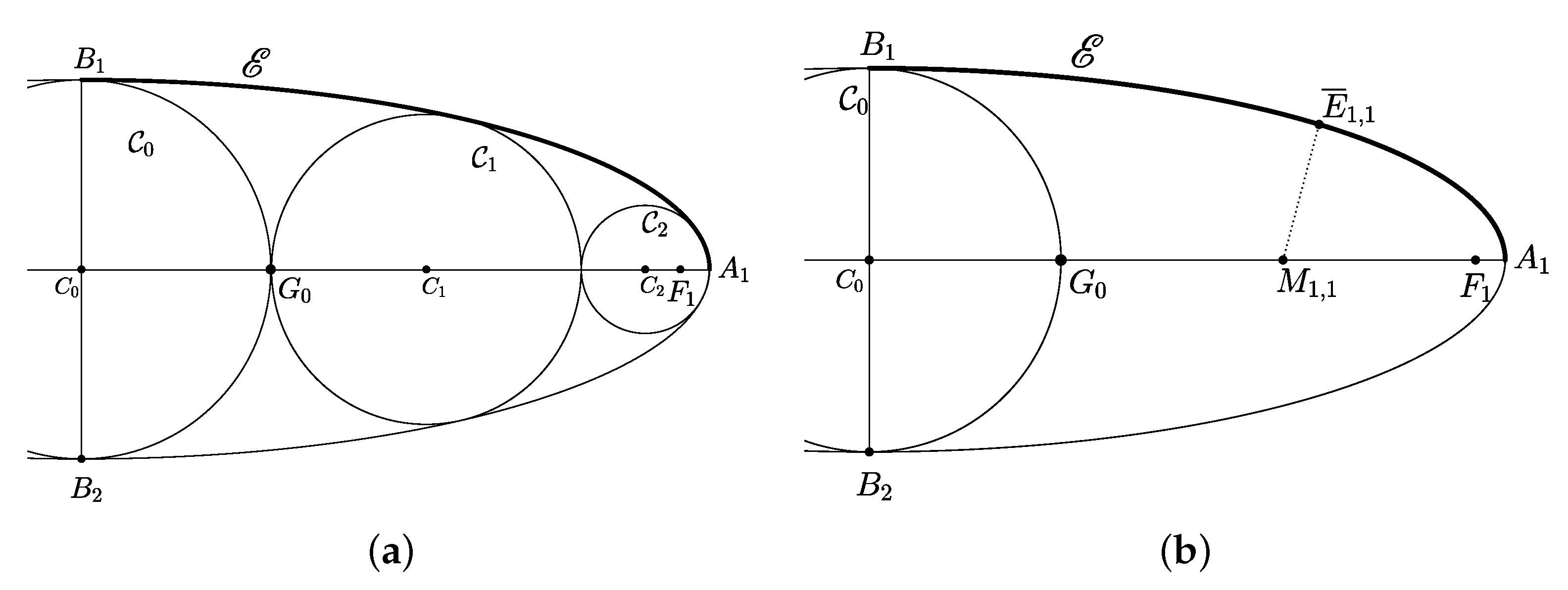
The construction of the scaffolding may be reduced to the construction of a discrete sequence of N 1 mutually externally tangent circles C n , shown in Figure 3a, internally tangent to ellipse E , having centers C n placed on the G 0 A 1 portion of ellipse semi-axis O A 1 and having decreasing radii r n .
We suppose the ellipse to be centered at the origin of a Cartesian reference frame. Scaffolding circle centers C n ( x n ; y n ) belong to the x-axis; thus, y n = 0 and may only be identified by means of their abscissa value, x n . The geometrical layout is shown in Figure 3b. The abscissa value of center C 1 of circle C 1 is a positive quantity and can be determined by applying a simple bisection algorithm. Each iteration of the algorithm monotonically reduces the indeterminacy interval length for abscissa x C 1 , providing better approximation C 1 i of center C 1 and better approximation for tangency condition C 1 G 0 ¯ = d ( C 1 , E ) .
The core part of the algorithm consists in choosing, as indeterminacy interval for center C 1 , segment G 0 A 1 ¯ ; as the first approximation of point C 1 , midpoint M 1 , 1 of segment G 0 A 1 ; and as the first approximation of the radius, value r 1 , 1 = M 1 , 1 G 0 ¯ = x M 1 , 1 x G 0 . By checking condition M 1 , 1 G 0 ¯ d ( M 1 , 1 , E ) , the indeterminacy interval may be restricted to segments G 1 M 1 , 1 or M 1 , 1 A 1 , respectively, and the algorithm may be reiterated.
The algorithm for the determination of center C n and radius r n of circle C n of the scaffolding is described in the following:
  • Quantity D n = k = 0 n 1 r k is evaluated, representing the abscissa of point G n 1 .
  • The first guess of radius r n of circle C n is set to be δ : = a D n (where the : = symbol indicates value storage in a variable).
  • Indeterminacy interval [ x m i n ; x m a x ] for coordinate x C n of center C n is initialized as x m i n : = x G n 1 and x m a x : = x A 1 .
  • The approximation of abscissa x C n is midpoint abscissa x M : = ( x m + x M ) / 2 .
  • Two consecutive approximations of the value of radius r n are stored in two variables, δ 0 : = δ and δ : = x M D n .
  • If δ < d ( M , E ) , then x m a x : = x M .
    if δ > d ( M , E ) , then x m i n : = x M .
  • The algorithm is terminated if the difference between current-step approximation δ and previous-step approximation δ 0 is less than predefined accuracy ε t n g ; otherwise, steps 4–6 of the algorithm are reiterated.

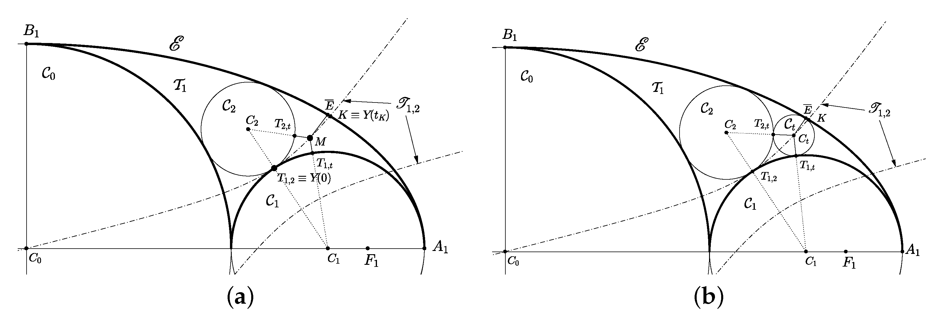
2.3. Tangent Circles in the Elliptic Domain

In the pursue of the circle packing, we will adopt the following terminology: Three given mutually tangent circles C 0 , C 1 and C 2 delimiting a curvilinear triangular region T 0 , 1 , 2 , will be referred to as stem circles. By applying Equations (3) and (4) to stem circle centers and radii, a  new circle C 3 that is internal to T 0 , 1 , 2 and tangent to the stem circles may be found; such circle will be referred to as the sprout circle.

2.3.1. The Search for the Solution by Means of Menaechmics
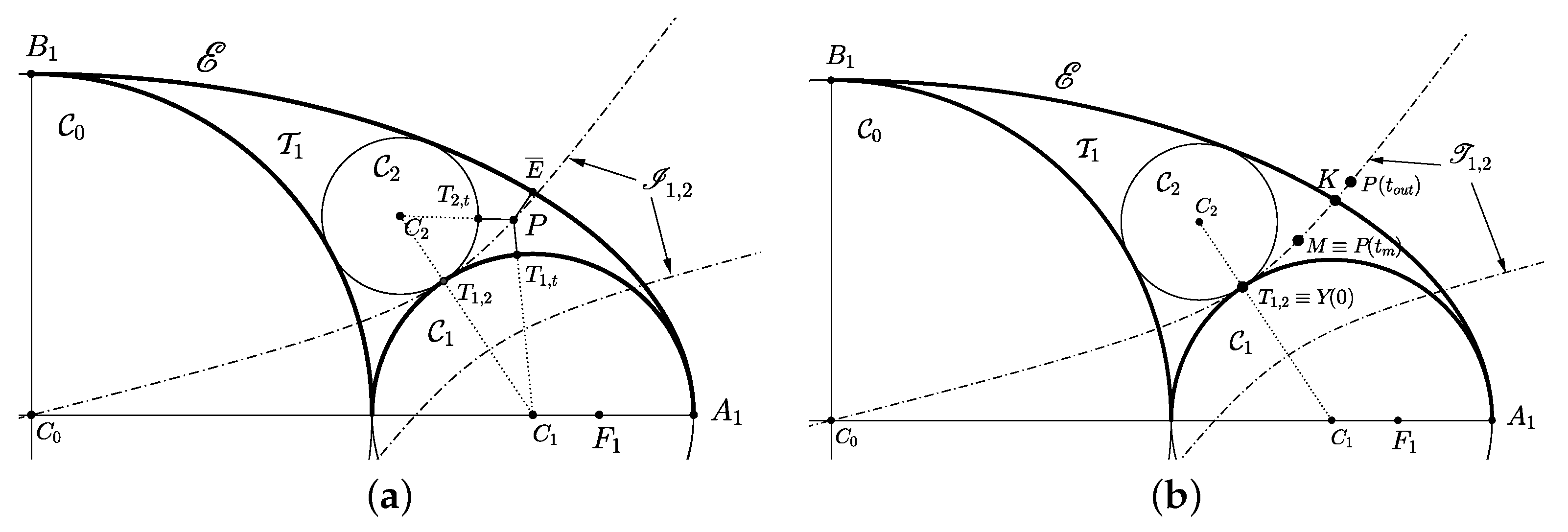
A specific algorithm must be devised for the search for sprout circles of the packing that are externally tangent to two stem circles and internally tangent to elliptic boundary E . Figure 4a depicts a typical geometric layout resulting from the packing procedure applied to the scaffolding shown in Figure 1b. The search for a circle C t that is externally tangent to circles C 1 and C 2 and tangent to elliptic boundary E may be reduced to the problem of constructing a point P that is internal to the arbelos-shaped curvilinear triangle T 1 and placed at equal distance from the boundaries of C 1 , C 2 and E . By identifying the centers and radii of circles C 1 , C 2 by means of symbols C 1 , r 1 , C 2 and r 2 , respectively, such properties may be translated into the following relation:
P T 2 , t ¯ = P T 1 , t ¯ = d ( P , E )
where T 1 , t and T 2 , t are the tangency point between circles C 1 and C 2 , and circle C t .
By expressing distances in terms of radii,
P T 2 , t ¯ = P C ¯ 2 r 2 P T 1 , t ¯ = P C ¯ 1 r 1
By separating the two equalities in Equation (5) and rearranging the terms, we obtain
P C ¯ 1 P C ¯ 2 = r 1 r 2 ( 7a ) P C ¯ 2 r 2 = d ( P , E ) ( 7b ) P C ¯ 1 r 1 = d ( P , E ) ( 7c )
Equations (7a)–(7c) imply the following conditions, illustrated in Figure 4:
  • Center P belongs to hyperbola I 1 , 2 defined by Equation (7a) having foci C 1 and C 2 , and a minor semi-axis length r 1 r 2 .
  • Point P must be placed at a known distance from ellipse E , defined by Equation (7b) or Equation (7c).
It is easy to observe that tangency point T 1 , 2 of circles C 1 and C 2 belongs to hyperbola I 1 , 2 . In fact, T 1 , 2 C 1 ¯ = r 1 and T 1 , 2 C 2 ¯ = r 2 , and by subtracting these two relations,
T 1 , 2 C 2 ¯ T 1 , 2 C 1 ¯ = r 1 r 2 ,
thus T 1 , 2 satisfies Equation (7a).
A purely numerical approach to the solution of the tangency problem under analysis may be easily accomplished. Point P belongs to an hyperbola branch; thus, its coordinates may be expressed in dependence of a single real parameter t. The desired solution may be achieved by varying P ( t ) according to a convergent algorithm until the condition
P C 2 ¯ r 2 = P C 1 ¯ r 1 = d ( P , E )
is satisfied.

2.3.2. Parametrization of the Hyperbola

The geometrical tangency problem has been reduced to the determination of hyperbola I 1 , 2 having foci in centers C 1 and C 2 and passing through tangency point T 1 , 2 of circles C 1 and C 2 . A parametrization of hyperbola I 1 , 2 suitable for our purposes must take into account the general case, shown in Figure 4a, in which the hyperbola is defined by any two points F 1 and F 2 of the plane (with r 1 representing centers C 1 and C 2 ) and by a real number r 1 such that r 1 < F 1 F 2 ¯ (representing the radius length of circle C 1 ). The r 1  number defines a point T, on segment C 1 C 2 , such that T C 1 ¯ = r 1 (with T representing tangency point T 1 , 2 between circles C 1 and C 2 ). In Appendix A, details are given for the complete derivation of parametrization formulas for a point P ( x P , y P ) of the hyperbola, which result to be
x P = x T ± a cos φ cosh t b sin φ sinh t , y P = y T ± a sin φ cosh t b cos φ sinh t
where
a = r 1 , b = c 2 a 2 , c = F 1 F 2 ¯ / 2 , φ = arctan y 2 y 1 x 2 x 1
x C = ( x 1 + x 2 ) / 2 , y C = ( y 1 + y 2 ) / 2 , F 1 ( x 1 ; y 1 ) , F 2 ( x 2 ; y 2 ) .
The hyperbola branch may be chosen by means of the ± sign, and the formula for tangency point T results to be
x T = x 1 + k ( x 2 x 1 ) , y T = y 1 + k ( y 2 y 1 ) , k = r 1 2 c .

2.3.3. Determination of the Intersection Point

In the following subsection, a method is proposed for the determination of circle C t , shown in Figure 5a, which makes use of intersection point K between elliptic boundary E and the semi-branch of hyperbola I 1 , 2 , passing through region T 1 . The geometric layout of the problem is shown in Figure 4b. The search for intersection point K may be carried out by means of a discrete sequence of approximations K i ( i N ) generated by a bisection algorithm, provided that an initial guess for the indeterminacy interval of point K is made and that the internal–external test, determining whether a point P is internal or external to elliptic boundary E , is conducted. Given an elliptic boundary E , enclosing an elliptic domain ε , having semi-axis lengths a and b,
P ( t ) = P x P ( t ) ; y P ( t ) , σ = x P 2 a 2 + y P 2 b 2 P ε E if σ > 0 P E if σ = 0 P ε if σ > 0
The essence of the algorithms consists in finding a value t o u t corresponding to a point P o u t = P ( t o u t ) on the hyperbola branch outside ε . The indeterminacy interval for point K is represented by hyperbola arc T 1 , 2 P o u t , and the first approximation of point K is point M, corresponding to the mean value between t = 0 and t = t o u t . By testing if point M is internal or external to ε , the  indeterminacy interval for K may be restricted, and a better approximation of K may be found. The algorithm is reiterated until desired accuracy ε i n t is obtained.

2.3.4. Determination of the Tangent Circle Center and Radius

The search for circle C t , shown in Figure 5a, which is externally tangent to circles C 1 and C 2 and internally tangent to elliptic boundary E , may be carried out by means of a bisection algorithm, restricting the indeterminacy position interval for circle center C t . The first guess for the indeterminacy interval for point C t is hyperbolic arc T 1 , 2 K , with  T 1 , 2 being the tangency point between circles C 1 and C 2 , and K being the intersection point between ellipse E and hyperbola I 1 , 2 found in the previous subsection. The first approximation of point C t is represented by point M, corresponding to the mean value between values t = 0 (point T 1 , 2 ) and t = t K (with P ( t K ) being the best approximation of point K). Then, condition M C 2 ¯ r 2 = M C 1 ¯ r 1 d ( M , E ) is tested by checking the equidistance of M from boundaries C 1 , C 2 and E , as stated in Equation (9). By means of such condition, the indeterminacy interval for point C t may be restricted to the first half or the second half of the interval, and a better approximation of C t may be found. The algorithm is reiterated until the desired accuracy for center C t is obtained, i.e., when the difference between the distance of point M from C 1 (or C 2 ) and ellipse E is less than predefined accuracy ε t n g : ( M C 2 ¯ r 2 ) d ( M , E ) = ( M C 1 ¯ r 1 ) d ( M , E ) < ε t n g , and circle C t , shown in Figure 5b, may be drawn.

2.4. Covering the Ellipse

Once the solution of the circle tangency problem is achieved, a proper orderly sequence of circle constructions must be devised, defining a suitable circle-packing algorithm for the complete filling of the planar domain. Using methods exposed in the previous sections, we are able to pack a sprout circle C t into a curvilinear triangle T a , b , c enclosed between three mutually tangent circles or between two tangent circles and outer elliptic boundary E . To  further proceed with the packing procedure, the same sprout circle C t , together with any possible couple of its stem circles, defines three new sets of stem circles and three new curvilinear triangular regions, T t , a , b , T t , a , c and T t , b , c . By iteratively or recursively finding the three sprout circles in these new regions, complete packing is achieved.

2.4.1. Data Structure: The Circle Array for the Elliptic Domain

The numerical implementation of the above packing algorithm may be pursued by means of a suitable data structure and relative representation. Owing to the straightforward character of the circle construction sequence, a simple data structure represented by means of an array is sufficient for our purposes.
In Table 1, the structure of the circle array (CA) is shown in a typical setting of its elements’ values at the starting point of the algorithm, i.e., when the N scaffolding circles and planar domain T 1 , shown in Figure 1a and Figure 2b, are defined. Circles are addressed by means of the first index (row index n) of the array, and elementary information regarding a single circle are stored in the elements of a row and may be addressed by means of the second index (column index m) of the array; thus, a single element of the CA is indicated with the C A ( n , m ) symbol. In particular:
  • The first three columns of the n-th row of the array, C A ( n , 1 ) , C A ( n , 2 ) and C A ( n , 3 ) , contain center coordinates x n and y n , and radius length r n of the n-th circle, respectively.
  • The second three columns of the n-th row of the array, C A ( n , 4 ) , C A ( n , 5 ) and C A ( n , 6 ) , are the stem pointers of the n-th circle and contain indexes p n , p n and p n of the three rows containing information (center coordinates and radius lengths) about the three stem circles generating the n-th circle; the presence of special value 1 in one of these columns indicates that the n-th circle is tangent to ellipse boundary E .
  • The second last column of the n-th row of the array, C A ( n , 7 ) , contains a flag value, f n ; this flag is set to 1 if the n-th circle must give way to further generation of sprouts circles, and it is set to 0 if further generation of sprouts circles originating from the n-th circle must be terminated.
  • The last column of the n-th row of the array, C A ( n , 8 ) , contains the value of the x coordinate of the tangency point between the n-th circle and ellipse boundary E ; such value is used to easily define the arcs to which the point-to-ellipse algorithm is applied.
The second three columns of the first N rows, referring to scaffolding circles, are not used by the algorithm and may thus be set to either 1 or 0. Starting from the first N rows of the CA, as the packing algorithm is applied, further rows of the CA are defined.

2.4.2. Implementation of the Packing Algorithm

Iterative Version of the Algorithm

The packing algorithm was implemented in Matlab®. The core element of the implementation is a subfunction, EllipseSprout(n1,n2,n3,CA), which obtains, as input arguments, three values of row index n of the CA and produces the effect of adding a new row, n s , to the CA containing information about the new sprout circle generated by stem circles stored in rows n 1 , n 2 and n 3 . The subfunction performs an initial test by controlling the presence of the conventional index value (i.e., value 1 ) in any of its first three parameters, n 1 , n 2 and n 3 , indicating that one of the stems of the circle under analysis is actually boundary ellipse E , thus determining whether to apply the Descartes complex formula given in Equation (4) or the ellipse tangency algorithm described in Section (Section 2.3) to compute the center and radius of the new sprout circle to be stored in a new row of the CA with index n s . If radius r s of the new sprout circle is smaller than specified amount r m i n , then flag f n s of row n s is set to 0.
At the beginning of the procedure, N 1 instances of the EllipseSprout function are launched, i.e., EllipseSprout(-1,n,n+1) for n = 0 , , N 2 , resulting in the determination of new circles internally tangent to the elliptic boundary (corresponding to value 1 as the first input parameter) and externally tangent to two consecutive circles of the scaffolding (corresponding to the two consecutive row indexes as the second and third input parameters). Information about these new “first generation” sprout circles is stored in N 1 additional rows of the CA having index n = N , , 2 N 1 .
The EllipseSprout function is subsequently launched to compute all “second generation” sprout circles generated by the N 1 first-generation circles, starting from the array row of index 2 N and proceeding to compute the sprout circles defined by the n-th circle by means of its stem circle pointers, provided that its flag f n has a non-zero value. Iteratively, the EllipseSprout function is subsequently launched to compute all “next-generation” sprout circles generated by “previous-generation” circles having non-zero f n flag values, thus accomplishing complete Apollonian packing within the elliptic domain to desired accuracy r m i n .

Recursive Version of the Algorithm

Alternatively, the algorithm may be expressed in a recursive form. In this case, the core element of the implementation is a recursive subfunction, EllipseSproutRec(n1,n2,n3,CA), which obtains, as input arguments, three values of row index n of the CA and produces the effect of adding a new row, n s , to the CA containing information about the new sprout circles.
The basic step of the EllipseSproutRec function is the determination of a new sprout circle generated by stems with indexes n1, n1 and n3 and the storage of its relevant information in the new row of the CA with index n4.
Subsequently, the EllipseSproutRec function tests the flag f 4 value, determining whether termination or recursion should occur:
  • If flag f 4 has a zero value, execution of the function is terminated.
  • If flag f 4 has a non-zero value, the function performs three recursive calls to generate the “further-generation” circles generated by circle n 4 , together with any two of its stems: 
    -
    EllipseSproutRec(n4,n1,n2,CA).
    -
    EllipseSproutRec(n4,n1,n3,CA).
    -
    EllipseSproutRec(n4,n2,n3,CA).
At the beginning of the packing procedure, N 1 instances of the EllipseSproutRec function are launched, i.e.,  EllipseSproutRec(-1,n,n+1,CA) for n = 1 , , N 1 . The resulting self-activated recursive sequence of instances provides the creation of rows of the CA, achieving complete Apollonian packing within the ellipse to desired accuracy r m i n .

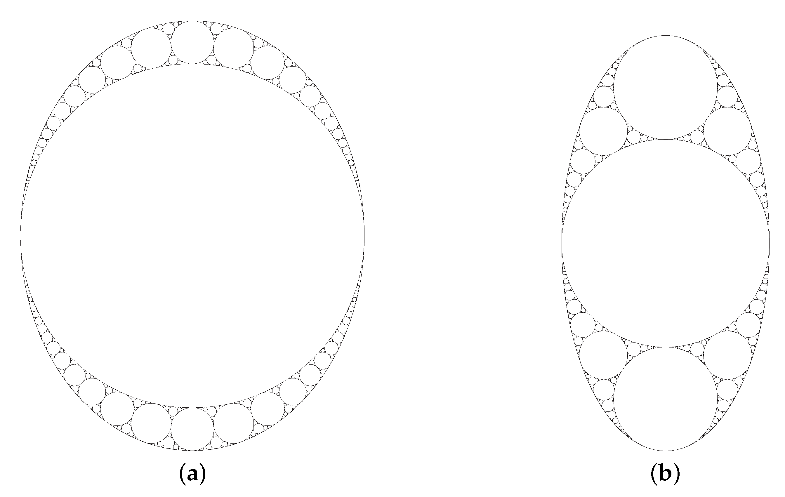
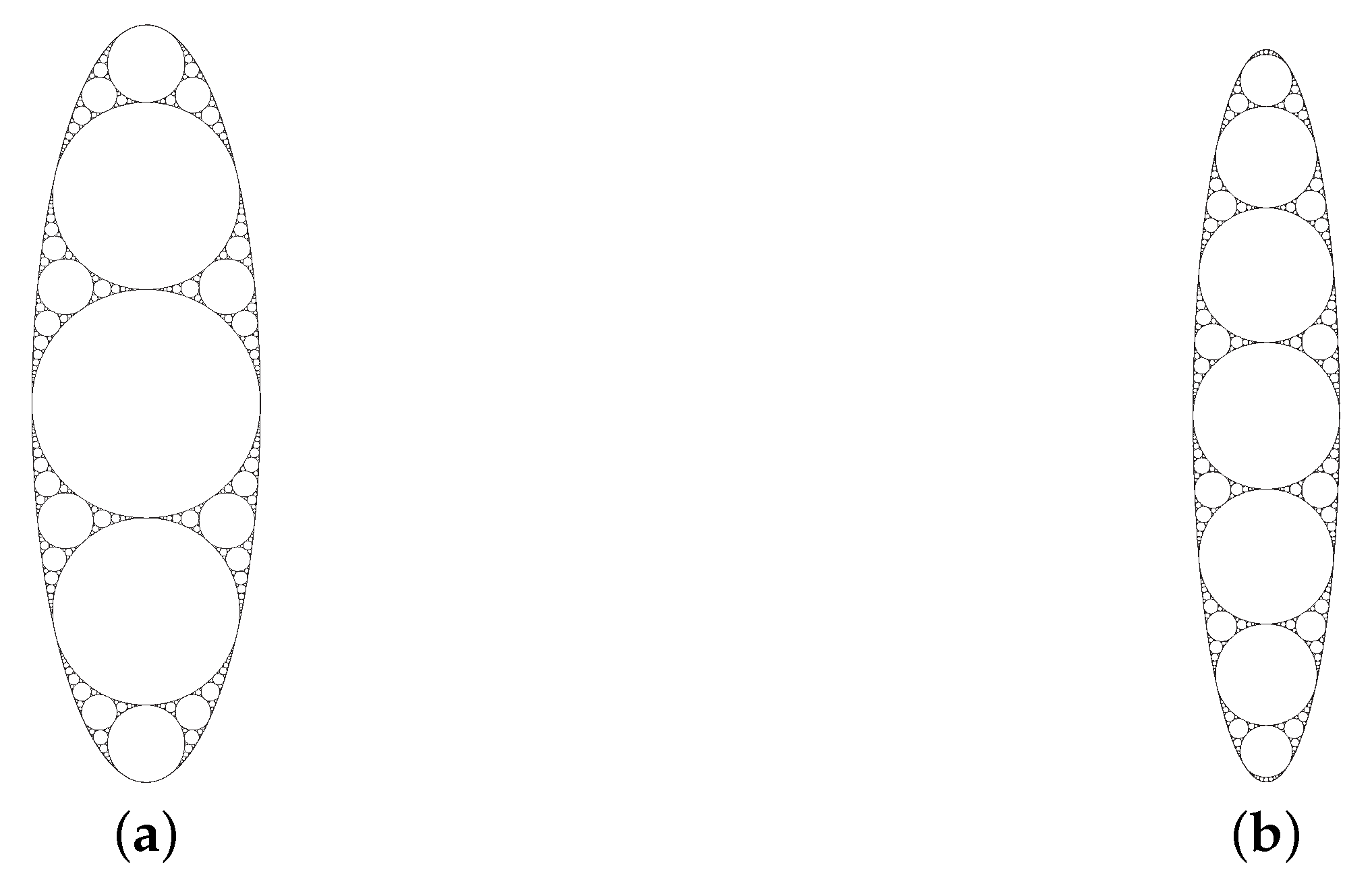
3. Results and Discussion

In Figure 6 and Figure 7, the results of the Apollonian packing procedure, implemented in Matlab®, are shown for the cases of a / b = 5 / 4 (Figure 6a), a / b = 2 (Figure 6b), a / b = 11 (Figure 7a) and a / b = 5 , (Figure 7b). In all the figures, r m i n = a / 150 . The results attest to the good accuracy and reliability of the proposed algorithm for a wide range of values of the eccentricity of the elliptic boundary.
The figures show evidence of the recursive nature of the branching sequence of circle filling in the elliptic domain, resulting in Sierpinski-like fractal morphogenesis [23]. The choice of simple, highly symmetrical scaffolding initial configurations, especially in the case of low-eccentricity ellipses, e.g., the structure shown in Figure 6a, fosters a reduction in the number of packing circles for a predefined filling accuracy; this choice would reasonably minimize computational complexity in simulations of the electromagnetic scattering of waves by elliptic-cross-section cylindrical structures assembled as a juxtaposition of circular cylindrical scatterers. The results might be easily applied to the modeling of physical fractals [24], allowing the circle radius distribution and the relevant fractal dimension to be numerically studied [25]. Similarly, Apollonian circle packings within non-circular boundaries could find interesting applications in space-filling bearings in connection with the study of tectonics and turbulence modeling [26]. A further analogy may be recognized between the presented structures and the covering of hierarchical nanostructures [27,28], the tiling of tubular nanostructures or other nanostructure modeling [29,30,31].

4. Conclusions

In this paper, an algorithm for the Apollonian circle packing within an ellipse is described. The algorithm has been implemented in a specific code to provide suitable testing, and although the algorithm was applied so as to give rise to simple structures that show symmetry with respect to the ellipse axes for illustrative purposes, it is suitable to achieve non-symmetric packing. The proposed method is based on fundamental numerical techniques and data structures, providing easy implementation, high accuracy and high stability in all cases. Owing to the generality of the numerical algorithms that have been employed, the method is suitable to be extended to the circle packing of any plane domain enclosed in any convex regular curve, if the suitable parametrization of the boundary is given. In the case of large-structure packing or a large number of algorithm iterations for optimization purposes, the development of specially devised methods to speed up the numerical evaluation of the point-to-boundary distance or the hyperbola–boundary intersection might turn out to be necessary, although strictly dependent on the analytical expression of the boundary curve. The proposed method is likely to undergo generalization to the three-dimensional case.

Author Contributions

Conceptualization, C.S., F.M. and F.F.; methodology, F.M. and F.F.; software, C.S. and F.M.; formal analysis, C.S.; investigation, C.S. and F.M.; writing—original draft preparation, C.S.; writing—review and editing, C.S., F.M. and F.F.; visualization, C.S.; supervision, F.F. All authors have read and agreed to the published version of the manuscript.

Funding

This research received no external funding.

Data Availability Statement

Not applicable.

Acknowledgments

The authors wish to thank Nicola Tedeschi for helpful discussions.

Conflicts of Interest

The authors declare no conflict of interest.

Appendix A. Deduction of Hyperbola Parametrization Formulas

Appendix A.1. Parametrizaton in the Canonical Reference Frame

A simple example of parametrization for the coordinates of a point P ( x P , y P ) belonging to any of the two branches of a hyperbola in the canonical reference frame shown in Figure A1a is the following:
x P = ± a cosh t , y P = b sinh t
where t is the real parameter, and a and b are two positive real numbers representing the hyperbola real and imaginary semi-axis lengths, respectively. The + sign is chosen to parametrize the right branch of the hyperbola, made of points with positive abscissas, while the − sign parametrizes the left branch.
Figure A1. (a) Hyperbola in the canonical reference frame and (b) after rotation by an angle φ . (c) Hyperbola after rototranslation.
Algorithms 16 00129 g0a1

Appendix A.2. Parametrization in the General Case

Parametrization formulas may be deduced by expressing point coordinates as complex coordinates and by applying rototranslation to the hyperbola in the canonical reference frame. A point P of hyperbola I in the canonical reference frame is identified by the following complex number:
z P = x P + i y P = a cosh t + i b sinh t ,
In Figure A1b, the first step of the transformation to the general form is shown. Rotation by an angle φ is applied, and a transformed hyperbola I is obtained. In the final arrangement, focal line F 1 F 2 is tilted by angle φ with respect of the x-axis; thus, since foci F 1 and F 2 are identified by complex numbers z 1 = x 1 + i y 1 and z 2 = x 2 + i y 2 , respectively,
φ = Arg ( z 1 , 2 ) , z 1 , 2 = z 2 z 1 .
From Equation (A3) and usual relations between hyperbola focal distance and axis length, Equation (11) is obtained. Point P of the hyperbola is transformed into point P ( x P , y P ) , corresponding to the following complex number:
z P = x P + i y P = e i φ z P = ( cos φ + i sin φ ) ( a cosh t + i b sinh t ) = = ± a cos φ cosh t b sin φ sinh t + i ± a sin φ cosh t b cos φ sinh t
Subsequently, translation is applied, transforming midpoint O ( 0 ; 0 ) into point C, the midpoint of segment F 1 F 2 , corresponding to complex number z C = ( z 1 + z 2 ) / 2 , giving rise to Equation (12). In Figure A1c, the last step of the transformation to the general form is shown. Point P of hyperbola I is transformed into point P ( x P ; y P ) of translated hyperbola I , corresponding to the following complex number:
z P = x P + i y P = z C + Z P = ( x C + i y C ) + ( x P + i y P ) = = x C ± a cos φ cosh t b sin φ sinh t + i y C ± a sin φ cosh t b cos φ sinh t .
By separating real and imaginary parts, Equations (10) is obtained.
Coordinates z R of a point R F 1 F 2 may be expressed by means of the following parametrization:
z R = ( 1 k ) z 1 + k z 2
which conveys R F 1 for k = 0 and R F 1 for k = 1 ; for any R, k = F 1 R ¯ / F 1 F 2 ¯ .
Point A 1 F 1 F 2 is defined by number r 1 = A 1 F 1 ¯ and corresponds to value k = A 1 F 1 ¯ / F 1 F 2 ¯ = r 1 / F 1 F 2 ¯ . By means of the last remark and by rearranging Equation (A6), Equation (13) is obtained.

Appendix A.3. Choice of the Correct Hyperbola Branch

By means of a suitable choice for the ± symbol and parameter t in Equation (A1), point P describes four semi-branches of hyperbola I , shown in Figure A1a. In particular:
  • By using the ± sign in the parametrization, point P ( t ) describes right branch I a or left branch I b .
  • By using values t 0 in the parametrization, point P ( t ) describes upper semi-branches I a + and I b + or lower semi-branches I a and I b .
In the search for circle C t , which is externally tangent to circles C 1 and C 2 and tangent to elliptic boundary E , it is necessary to pay particular attention to the choice of the suitable hyperbola semi-branch on which center C 1 must be searched for. By taking into careful considerations all possible arrangements of the tangency geometrical layout, a procedure for the choice of the hyperbola semi-branch may be described as follows:
  • In Equations (10)–(12), it is important to ensure that condition C C 1 ¯ = r 1 > r 2 = C C 2 ¯ is satisfied (i.e., C 1 must be the largest circle).
  • In Equations (10), only the + determination of the ± sign is used (i.e., only the right branch of I a is taken into consideration).
  • The negative sign for parameter t is chosen only in the two cases of φ > π / 2 or x T 1 > x T 2 , with T 1 and T 2 being the tangency points between boundary ellipse E and circles C 1 and C 2 .

References

  1. Castillo, I.; Kampas, F.J.; Pintér, J.D. Solving circle packing problems by global optimization: Numerical results and industrial applications. Eur. J. Oper. Res. 2008, 191, 786–802. [Google Scholar] [CrossRef]
  2. Birgina, E.G.; Bustamantea, L.H.; Callisaya, H.F.; Martınez, J.M. Packing circles within ellipses. Int. Trans. Oper. Res. 2013, 20, 365–389. [Google Scholar] [CrossRef] [Green Version]
  3. Holly, J.E. What Type of Apollonian Circle Packing Will Appear? Am. Math. Mon. 2021, 128, 611–629. [Google Scholar] [CrossRef]
  4. Herrmann, H.J.; Mantica, G.; Bessis, D. Space-filling bearings. Phys. Rev. Lett. 1990, 65, 3223–3226. [Google Scholar] [CrossRef] [PubMed]
  5. Herrmann, H.J.; Astrøm, J.A.; Mahmoodi Baram, R. Rotations in shear bands and polydisperse packings. Phys. A: Stat. Mech. Its Appl. 2004, 344, 516–522. [Google Scholar] [CrossRef]
  6. Soddy, F. The Kiss Precise. Nature 1936, 137, 1021. [Google Scholar] [CrossRef] [Green Version]
  7. Lagarias, J.C.; Mallows, C.L.; Wilks, A.R. Beyond the Descartes circle theorem. Am. Math. Mon. 2002, 109, 338–361. [Google Scholar] [CrossRef]
  8. McDonald, K. A Solution to the Problem of Apollonius. 1964. Available online: http://kirkmcd.princeton.edu/papers/apollonius_051964.pdf (accessed on 21 February 2023).
  9. Coxeter, H.S.M. Introduction to Geometry, 2nd ed.; John Wiley & Sons: Hoboken NJ, USA, 1969; pp. 77–90. [Google Scholar]
  10. Christersson, M. Apollonian Gasket. 2019. Available online: http://www.malinc.se/math/geometry/apolloniangasketen.php (accessed on 7 October 2022).
  11. Netz, R. Greek Mathematicians: A Group Picture. In Science and Mathematics in Ancient Greek Culture; Tuplin, C.J., Rihll, T.E., Eds.; Oxford University Press: Oxford, UK, 2002. [Google Scholar]
  12. Richmond, J.H. Scattering by an Arbitrary Array of Parallel Wires. IEEE Trans. Microw. Theory Tech. 1965, 13, 408–412. [Google Scholar] [CrossRef]
  13. Frezza, F.; Mangini, F.; Tedeschi, N. Introduction to electromagnetic scattering: Tutorial. J. Opt. Soc. Am. A 2018, 35, 163–173. [Google Scholar] [CrossRef] [PubMed]
  14. Frezza, F.; Mangini, F.; Tedeschi, N. Introduction to electromagnetic scattering, part II: Tutorial. J. Opt. Soc. Am. A 2020, 37, 1300–1315. [Google Scholar] [CrossRef] [PubMed]
  15. Frezza, F.; Mangini, F.; Muzi, M.; Stoja, E. In silico validation procedure for cell volume fraction estimation through dielectric spectroscopy. J. Biol. Phys. 2015, 41, 223–234. [Google Scholar] [CrossRef] [PubMed] [Green Version]
  16. Callisaya, H.F. Empacotamento em Quadràticas. Ph.D. Thesis, Institute of Mathematics, Statistics and Scientific Computing, University of Campinas, Campinas, Brasil, 16 March 2012. Available online: https://www.ime.unicamp.br/pos-graduacao/empacotamento-quadraticas (accessed on 7 October 2022).
  17. Nürnberg, R. Distance from a Point to an Ellipse. 2006. Available online: https://nurnberg.maths.unitn.it/distance2ellipse.pdf (accessed on 7 October 2022).
  18. Eberly, D. Distance from a Point to an Ellipse, an Ellipsoid, or a Hyperellipsoid. 2020. Available online: https://www.geometrictools.com/Documentation/DistancePointEllipseEllipsoid.pdf (accessed on 7 October 2022).
  19. Kiefer, J. Sequential Minimax Search for a Maximum. Proc. Am. Math. Soc. 1953, 4, 502–506. [Google Scholar] [CrossRef]
  20. Teukolsky, S.A.; Flannery, B.P.; Press, W.H.; Vetterling, W.T. Numerical recipes in C: The Art of Scientific Computing, 2nd ed.; Cambridge University Press: New York, NY, USA, 1992; pp. 397–402. [Google Scholar]
  21. Aharonov, D.; Stephenson, K. Geometric sequences of discs in the Apollonian packing. St. Petersbg. Math. J. 1998, 9, 509–542. [Google Scholar]
  22. Lawrence, J.D. A Catalog of Special Plane Curves; Dover Publications: New York, NY, USA, 1972; pp. 131–134. [Google Scholar]
  23. Bourke, P. An introduction to the Apollonian fractal. Comput. Graph. 2006, 30, 134–136. [Google Scholar] [CrossRef]
  24. Varrato, F.; Foffi, G. Apollonian packings as physical fractals. Mol. Phys. 2011, 109, 2663–2669. [Google Scholar] [CrossRef] [Green Version]
  25. Mauldin, R.D.; Urbański, M. Dimension and Measures for a Curvilinear Sierpinski Gasket or Apollonian Packing. Adv. Math. 1998, 136, 26–38. [Google Scholar] [CrossRef] [Green Version]
  26. Manna, S.S.; Herrmann, H.J. Precise determination of the fractal dimensions of Apollonian packing and space-filling bearings. J. Phys. A Math. Gen. 1991, 24, 481–490. [Google Scholar] [CrossRef]
  27. Shao, J.; Ding, Y.; Wang, W.; Mei, X.; Zhai, H.; Tian, H.; Li, X.; Liu, B. Generation of Fully-Covering Hierarchical Micro-/Nano- Structures by Nanoimprinting and Modified Laser Swelling. Small 2014, 10, 2595–2601. [Google Scholar] [CrossRef] [PubMed]
  28. Son, J.G.; Hannon, A.F.; Gotrik, K.W.; Alexander-Katz, A.; Ross, C.A. Hierarchical Nanostructures by Sequential Self-Assembly of Styrene-Dimethylsiloxane Block Copolymers of Different Periods. Adv. Mater. 2011, 23, 634–639. [Google Scholar] [CrossRef] [PubMed]
  29. Toffoli, H.; Erkoç, S.; Toffoli, D. Modeling of Nanostructures. In Handbook of Computational Chemistry; Leszczynski, J., Ed.; Springer: Dordrecht, The Netherlands, 2015; pp. 1–55. [Google Scholar]
  30. Diudea, M.V. Nanostructures: Novel Architecture; Nova Science Publishers: New York, NY, USA, 2005. [Google Scholar]
  31. Chandel, V.S.; Wang, G.; Talha, M. Advances in modelling and analysis of nano structures: A review. Nanotechnol. Rev. 2020, 9, 230–258. [Google Scholar] [CrossRef]
Figure 1. Scaffoldings for ellipses with a / b = 5 / 4 (a) and a / b = 2 (b).
Algorithms 16 00129 g001
Figure 2. Scaffoldings for ellipses with a / b = 11 (a) and a / b = 5 (b).
Algorithms 16 00129 g002
Figure 3. (a) Detail of the scaffolding in Figure 2a. (b) Determination of center and radius of circle C 1 shown in (a).
Algorithms 16 00129 g003
Figure 4. (a) Equidistance condition of point P from the surrounding boundaries. (b) Hyperbola expressing the condition of equidistance of point P from circles C 1 and C 2 .
Algorithms 16 00129 g004
Figure 5. (a) Determination of center C t of sprout circle C t and circle C t . (b) Packing of circle C t .
Algorithms 16 00129 g005
Figure 6. Apollonian packing for a / b = 5 / 4 (a) and for a / b = 2 (b). In both cases, r m i n = a / 150 .
Algorithms 16 00129 g006
Figure 7. Apollonian packing for a / b = 11 (a) and for a / b = 5 (b). In both cases, r m i n = a / 150 .
Algorithms 16 00129 g007
Table 1. Circle array structure.
Row IndexCenterCenterRadius1st Stem2nd Stem3rd StemFlagTangency
n x n y n r n p n p n p n f n x T n
000 r 0 1 0010
1 x 1 y 1 r 1 1 001 x T 1
2 x 2 y 2 r 2 1 001 x T 2
3 x 3 y 3 r 3 1 001 x T 3
N 1 x N 1 y N 1 r N 1 1 001a
Note: n N ; p n , p n , p n N { 1 } ; x n , y n , r n , “ x T n R ; f n { 0 , 1 } .
Disclaimer/Publisher’s Note: The statements, opinions and data contained in all publications are solely those of the individual author(s) and contributor(s) and not of MDPI and/or the editor(s). MDPI and/or the editor(s) disclaim responsibility for any injury to people or property resulting from any ideas, methods, instructions or products referred to in the content.

