Article

Low-Order Electrochemical State Estimation for Li-Ion Batteries

by
Higuatzi Moreno
1,† and
Alexander Schaum
1,2,*,†
1
Automation and Control Group, Kiel University, 24232 Kiel, Germany
2
Kiel Nano, Surface and Interface Sciences (KiNSIS), 24118 Kiel, Germany
*
Author to whom correspondence should be addressed.
These authors contributed equally to this work.
Algorithms 2023, 16(2), 73; https://doi.org/10.3390/a16020073
Submission received: 23 December 2022 / Revised: 17 January 2023 / Accepted: 19 January 2023 / Published: 28 January 2023

Abstract

:
Batteries are complex systems involving spatially distributed microscopic mechanisms on different time scales whose adequate interplay is essential to ensure a desired functioning. Describing these phenomena yields nonlinearly coupled partial differential equations whose numerical solution requires considerable effort and computation time, making it an infeasible solution for real-time applications. Anyway, having information about the internal electrochemical states of the battery can pave the way for many different advanced monitoring and control strategies with a big potential for improving efficiency and longevity. For such purposes, in the present paper, a combination of a low-order representation of the essential dynamics associated to the internal electrochemical mechanisms based on Dynamic Mode Decomposition for control (DMDc) is proposed to obtain an improved equivalent circuit model (ECM) representation with continuously updated parameters and combined with an extended Kalman Filter (EKF). The model-order reduction step extensively exploits the model structure, yielding a well structured low-order representation without artificial numerical correlations. The performance of the proposed method is illustrated with numerical simulations based on a well-established reference model, showing its potential usefulness in real-time applications requiring knowledge of the internal electrochemical states besides the state-of-charge.

1. Introduction

Nowadays, Lithium-ion batteries play a pivotal role in industrial applications both in mobile and stationary solutions. For all these applications it, is vital to monitor and control the operational conditions of Li-ion batteries in order to increase their life time, reduce hazardous situations and provide reliability to the user ([1,2,3]). The state-of-charge (SOC) is one of the most important but also delicate parameters to monitor, given that it determines the effective remaining power that can be supplied with the battery, but it depends on the concentration distribution of charges in the electrode particles. Given this dependency it is not directly measurable, and thus is typically estimated from measurable output signals and known inputs on the basis of some mathematical or numerical model.
While batteries are intensively used in different applications, there are also still a couple of open questions requiring additional research and development. Li-ions batteries are complex systems involving spatially distributed microscopic mechanisms with nonlinear coupling effects on different time scales [4]. There is not a unique model representing all mechanisms but rather several models have been created, and even new ones are appearing, in an effort to model, predict and control the internal electrochemical processes that conform a Li-ion battery. In general, two main groups of models can be distinguished: electrochemical models based on first-principles (i.e., electrochemical reaction kinetics, mass and energy balances) and data-driven models.
The models based on first-principles incorporate the different chemical, electrical and physical factors into mathematical equations to predict the main internal phenomena as accurate as possible, see, e.g., [5,6,7,8,9,10,11,12,13]. These models have been used mainly to improve the understanding of the underlying mass transport and electrochemical kinetics phenomena on a quantitative-qualitative level. They have been validated in many independent experimental studies and their potential use in (i) state estimation for monitoring, (ii) optimal charging, and (iii) state feedback control design have been investigated by different groups (see, e.g., [14,15,16,17,18,19]). While these studies on the one side outline the great advantages of having explicit information about the internal electrochemical states at hand, on the other side they involve complex and advanced analytical skills and typically still require a complete partial differential equation system to be solved online, what can lead to significant real-time limitations and impose a high computational burden that is undesired in particular for embedded solutions and becomes untractable when concerning distributed battery packs and the associated complex battery management systems [20]. The simplest of the first-principle models is the so-called equivalent circuit model (ECM), (see, e.g., [21,22]), which can be used in fast simulation scenarios but neglects all internal electrochemical processes and in consequence has a lower prediction capability, typically showing offsets in comparison to detailed numerical models.
Because of the above other approaches are being explored in order to find a balance between a detailed electrochemical representation, simplicity and real-time capability. The data-driven modeling approaches offer such a balance. Data-driven modeling treats the battery basically as a black box and through model trainings comes up with a representation of the behaviour of the battery by using algorithms that process the measured data and iteratively improve the prediction capability. As a result, minimal or zero knowledge of the battery internal parameters is needed. Neural networks and deep learning are being used to form a relation between the input information and the output measurement (see, e.g., [23]). Moreover, these approaches are popular because they allow to improve the prediction by diverse paths of model training. Other approaches, such as support vector machines and fuzzy logic present attractive low-error representations of essential information due to their classification and regression methods. The different advantages of first-principles and data-driven modeling approaches can be found in [24]. What should be highlighted here is that any method that only considers input–output data, even treating hidden dynamics by means of lateral variables can not be verified with respect to the internal electrochemical state predictions, unless it is compared-during training-to detailed first-principle models, which at this moment are the main source of information about what happens inside the battery.
This motivates to focus on different systematic model simplification and model order reduction techniques. This has been addressed, e.g., using singular perturbation approaches [4], numerical approximation using, e.g., finite-differences and averaging [25,26], frequency domain approaches coupled with low-order state space models [27] and Galerkin projections [28,29], polynomial projections [30] and others (see, e.g., [31]). A further powerful tool for low-order model identification has been gaining importance in different application fields due to its capacity to systematically identify low-dimensional relations of complex systems in discrete-time setups using snapshots of the states, namely Dynamic Mode Decomposition (DMD) [32,33] and its extensions to include external control inputs, known as Dynamic Mode Decomposition with control (DMDc) [34]. Having in its core singular value decomposition and Koopman operator theory [35], DMDc has shown a big potential use in fields ranging from the analysis of turbulent flows [32,35,36] to shallow water propagation in channels [37]. Accordingly, it is to be expected that DMDc also provides an excelent basis for low-order prediction model approximations for batteries, using which one can determine the essential (i.e., dominant) modes that govern the electrochemical dynamics and create a reduced order model (ROM) on this basis, which inherits not only the accuracy of the detailed model but is also simple enough to be used in real-time applications.
DMDc was recently used for battery model identification [38] with a restriction on the consideration of input–output and SOC data but without any relation to the electrochemical dynamics within the cell. In contrast to this, a ROM based on a detailed electrochemical model and obtained via DMDc was proposed in [39]. In a similar fashion as for the other model-order reduction techniques commented above, the main advantage relies in the fact that essential effects of the electrochemistry can still be represented and explicitely considered, paving the way, e.g., for monitoring and control applications based on the electrochemical state information. An advantage of DMDc from the application point of view is that the choice of functions on which the dynamics are projected takes place automatically on the basis of the data, i.e., the snapshots of the states, obtained either from measurements or from simulations, while in the other mentioned model-order reduction techniques the associated analytical effort is considerably higher.
Independent of the method, any prediction model is just an approximation and thus monitoring and control approaches require some estimator, providing a correction of the predictions on the basis of measured data. For such purposes, basically two main groups of approaches can be found: observers based on deterministic system equations [11,14,40,41,42] and estimators for stochastic system representations [43].
Within classical methods for the estimator design, the Kalmal filter (KF) is a well known tool for stochastic linear systems, and the extended Kalman filter (EKF) for non-linear systems. The EKF uses the nonlinear model for prediction and a local linearisation about the current estimate to predict the associated error covariance in dependence of measurement and process noise covariances, to achieve a local minimization of the estimation error covariance. Kalman Filter methods have already been applied by different groups to battery models, see, e.g., [22,25,44]. Besides these classical Kalman Filter approaches, e.g., particle filters (PF) and Adaptative Extended Kalman filter (AEKF) have also been used to predict the SOC in data-driven models but considering only the experimental and measurable outputs obtained from physical set-ups, leaving aside the underlying electrochemical behaviour (see, e.g., [45,46,47]). The combination of DMDc with Kalman filtering techniques has also been discussed in several studies (see, e.g., [48,49,50,51,52,53]), given that both are very systematic and easily implementable methods providing a high degree of precission and efficiency.
Having the above mentioned studies as points of departure, the purpose of the present study is to (i) extend the ROM proposed in [39] to include thermal dynamics, (ii) use the improved ROM for time-variant adaptation of the parameters of an ECM, and (iii) combine it with an EKF for estimation of microscopic (i.e., electrochemical) and macroscopic (i.e., voltage-current, SOC) states. The performance of the proposed estimation scheme is established by simulation studies with a comparison to a high-fidelity numerical solution of a detailed electrochemical model [9,54], in order to show the approximation quality achieved with the DMDc based ROM in combination with the EKF.
The paper is organized as follows: First, in Section 2, the methodology is presented with a review of the mathematical equations of the single particle electrode model. This is followed by a derivation of the numerical model obtained by the solution through a finite difference scheme. Then DMDc is recalled and applied to the battery model to derive the ROM. In continuation, an ECM and its improvement by an adaptation scheme based on the ROM is presented. Section 3 includes simulation studies to show the performance of the proposed approach. Conclusions and an outlook are presented in Section 4 and Section 5, respectively.

2. Methodology and Models

For the present work, the model developed in [54] considernig a DUAL Li-ion battery with LiC 6 for the negative electrode, Li 2 Mn 2 O 4 for the positive electrode, and LiPF 6 as electrolyte is considered.

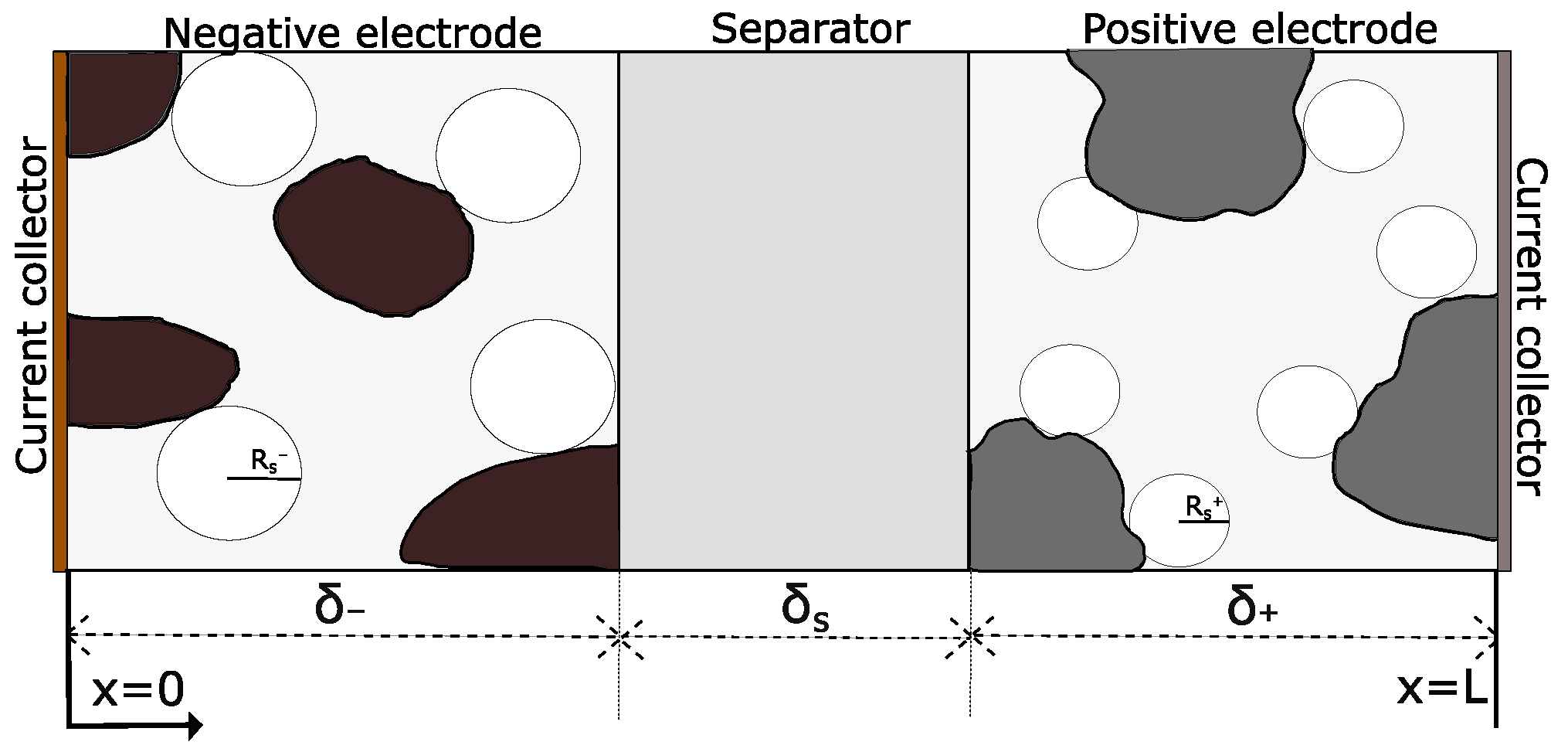
2.1. The Single Particle Model Revisited

The porous electrode theory for DUAL configuration, based on the work of Doyle and Newman, was chosen because it is general enough to be adapted to other batteries. To simplify the electron transport, the single particle model is used to provide an average interaction between the surface of the active material spheres and the electrolyte. Additionally, the simplified model still provides a deep understanding of the electrochemical interactions that occur on each electrode, in the electrolyte and the solid electrolyte interphase (SEI). The theory divides the Li-ion battery into: Solid phase (concerning the electrodes), electrolyte phase, and reaction rate (concerning the interaction of the input current, the current of the phases, temperature and the potential at the surface of the electrodes according to the Buttler-Vollmer kinetics [55]). Figure 1 shows a scheme of the DUAL configuration of the model.
The model equation for the different components are briefly summarized in the following (cp. [54]).
  • Solid phase
The lithium concentration in the electrode is governed by
C s ( r , x , t ) t = 1 r 2 r D s r 2 C s ( r , x , t ) r , t > 0 , r ( 0 , R s ) , x ( 0 , L )
with initial condition C s ( · , · , 0 ) = C s 0 and boundary conditions
C s ( r , x , t ) r = 0 , t > 0 , r = 0 , x ( 0 , L )
D s C s ( r , x , t ) r = j n ( x , t ) , t > 0 , r = R s , x ( 0 , L ) ,
where C s ( r , x , t ) is the lithium concentration in either of the electrodes, r is the radius in spherical coordinates of the electrode-sphere particle with maximum value R s , D s is the diffusion coefficient, and j n ( x , t ) is the pore-wall flux. Note that (1a) corresponds to a spherical diffusion equation under the assumption of angular homogeneity regarding the azimuthal and longitudinal directions.
The potential of the electrode is governed by
Φ s ( x , t ) x = I ( t ) i e ( x , t ) σ , t > 0 , x ( 0 , L )
with boundary conditions
Φ s ( x , t ) x = 0 , t > 0 , x { δ , δ + δ s }
Φ s ( x , t ) x = I ( t ) σ , t > 0 , x { 0 , L } ,
where Φ s ( x , t ) is the electrode’s potential, I ( t ) is the input current density, i e ( x , t ) is the electrolyte current and σ is the conductivity of the electrode.
  • Electrolyte phase
The lithium concentration in the electrolyte satisfies
C e ( x , t ) t = x D e C e ( x , t ) x + t e 0 ( x ) F i e ( x , t ) x + i e ( x , t ) F t e 0 ( x ) x , t > 0 , x ( 0 , L )
with initial condition C e ( · , 0 ) = C e 0 and boundary conditions
C e ( x , t ) x = 0 , t > 0 , x = 0 , L ,
where i e ( x , t ) is the electrolyte current, F is Faraday’s constant, ε is the volume fraction for each electrode, C e ( x , t ) , D e and t e 0 are the lithium concentration, diffusion coefficient and the transference number of the electrolyte, respectively.
The electrolyte current in turn is governed by
i e ( x , t ) x = F a s j n ( x , t ) x [ 0 , δ ] 0 x [ δ , δ + δ s ] F a s + j n ( x , t ) x [ δ + δ s , L ] , t 0
with the specific interfacial area of the single sphere-particle
a s ± = 3 ( 1 ε ) R s ± .
The potential of the electrolyte satisfies
Φ e ( x , t ) x = i e ( x , t ) κ + R T F 1 t e 0 ( x ) l n C e ( x , t ) x , t 0 , x ( 0 , L )
with the boundary condition
Φ e ( x , t ) = 0 x = 0 ,
where R is the universal gas constant, T the cell temperature, and κ the ionic conductivity of the electrolyte.
  • Reaction rate
The reaction rate equations basically are described by the Buttler-Vollmer kinetics [55] which can be written in the form
F j n ( x , t ) = 2 i o ( x , t ) sinh α F R T η ( x , t )
with
η ( x , t ) = Φ s ( x , t ) Φ e ( x , t ) U O C P ( C s ) F R f j n ( x , t )
i o ( x , t ) = r e f f F C s m a x C s s u r f α ( C s s u r f C e ) α ,
where i o ( x , t ) is the exchange current density (by insertion of electrodes), α is the transport coefficient from the negative and positive electrodes, η is known as the overpotential and depends of the Open Circuit Potential U O C P , electrode and electrolyte potential and the ohmic drop produced by the union of the electrode and the current collector where R f is the film resistance, r e f f is the rate constant of the anodic and cathodic directions of the reaction, C s m a x represents the maximum concentration of lithium at either electrode, and C s s u r f is the concentration at the surface of the electrode-sphere particle.
Note that the pore-wall flux can be averaged as:
< j n > = I ( t ) F a s + δ + for the positive electrode I ( t ) F a s δ for the negative electrode
and the output voltage can be found solving (5a) for each potential of the electrode surface and the relationship
V ( t ) = Φ s , s u r f + ( t ) Φ s , s u r f ( t ) .
  • Energy balance
The power transferred through the battery produces internal heat that is interchanged with the environment. As the thickness of the electrodes is small, temperature gradients that are perpendicular to them can be omitted. This results in the following simplified model for the thermal dynamics
ρ a v g C p d T ( t ) d t = I ( t ) V ( t ) + h 0 T a m b T ( t ) , t > 0 , T ( 0 ) = T 0 ,
where ρ a v g is the average mass per unit area, C p is the heat capacity, h 0 is the heat transfer coefficient and T a m b is the external or environmental temperature.

2.2. Numerical Model

The model consists of a combination of partial differential equations, ordinary differential equations (in the spatial coordinates) and the central nonlinear Buttler-Vollmer kinetics as a coupling relation. For the solution of this system of equations in the following the method of finite-differences is employed, going along standards in the related literature (see, e.g., [25,26,56]).
For this purpose the spatial variables are discretized by introducing x i = i Δ x , r j = j Δ r with i = 1 , , n , j = 1 , , m , with n , m N and the discretization steps Δ x , Δ r > 0 .
  • Electrolyte current
First of all, notice that equation (3c) can be solved analytically. Before and after the separator the current is the same, no additional boundaries conditions are needed:
i e ( x , t ) = I ( t ) δ x 0 x δ I ( t ) δ s < x < δ + I ( t ) I ( t ) δ + ( x δ δ s ) δ + x L .
  • Electrolyte concentration
Introducing the short-hand notation C e , i ( t ) = C e ( x i , t ) , and the vector
C e ( t ) = C e , 1 ( t ) C e , n ( t ) T ,
 Equation (3a) can be approximated as:
C e ˙ ( t ) = A C e C e ( t ) + b C e I ( t )
where the matrix A C e and the vector b C e are defined in Appendix A.
  • Electrolyte potential
In the same fashion, introducing Φ e , i ( t ) = Φ e ( x i , t ) and 
Φ e ( t ) = Φ e , 1 ( t ) Φ e , n ( t ) T ,
Equation (4a) can be approximated by using central differences as:
A Φ e Φ e ( t ) = b Φ e I ( t ) + C Φ e ln C e ( t )
where the matrices A Φ e , C Φ e and the vector b Φ e defined in Appendix A.
  • Electrode concentration
For the case of the solid phase, the concentration is approximated by considering a spatial homogeneity with respect to the x-direction. With the creation of the vector C s ( x , t ) = C s ( r 1 , x , t ) C s ( r m , x , t ) , Equation (1a) can be expressed as:
C ˙ s ( x , t ) = A C s C s ( x , t ) + b C s I ( t )
where the matrix A C s and the vector b C s are given in Appendix A.
  • Output voltage
The open circuit potential of each material is assumed to be known. Mathematical approximations for different materials can be found, e.g., in [6]. Considering (6) and the boundary condition (4b), the only unknown in (5a) is the surface potential which can be solved to obtain:
Φ s , s u r f ( t ) = R T α F asinh F j n ( t ) 2 i o ( t ) + U O C P ( C s ( t ) ) + F R f j n ( t ) + Φ e + ( t )
so that the terminal output in (7) can be computed.
  • Electrode potentials
Finally, (2a) can be analytically integrated to obtain the potentials across the electrodes by making use of the boundary conditions (2b) and (2c):
Φ s ( x , t ) = Φ s , s u r f I ( t ) σ x ± I ( t ) 2 σ δ x 2 , 0 x δ .
Here, the electrodes are considered as separated items, i.e., the equation starts at x = 0 , or x + = δ + δ s artificially set to zero, respectively.
  • State of charge
By considering the saturation point in the concentration of Li-ions in each electrode and the concentration’s profile over time, it is possible to estimate the SOC of each electrode independently.
Regarding the SOC, two types can be determined from the model:
  • Surface SOC, regarding only the surface of the particle:
    S O C s u r f ( t ) = C s , s u r f C s , m a x
  • Bulk SOC, which contemplates the spatial profiles of the whole spheres:
    S O C b u l k ( t ) = 3 δ ( R s ) 3 0 δ 0 R s r 2 C s ( x , r , t ) C s , m a x d r d x

2.3. Dynamic Mode Decomposition with Control

By providing the specific parameters to the numerical model, a simulation can be conducted. All the data are collected then into the so-called snapshots [32,33,34]. DMDc uses these snapshots together with the external signals (current and temperature) to approximate the input–output dynamics. For this purpose, consider the vector x k , conformed by stacking of all the electrochemical states defined in the mathematical equation of Section 2.1:
x k = C e Φ e C s Φ s C s + Φ s + T .
DMDc characterizes the relationship between the actual state x k , the future state x k + 1 and the external input u k  considering a linear discrete time dynamical system of the form
x k + 1 = A x k + B u k ,
where x k R n , u k R q , A R n x n , B R n x q and k [ 1 , M ] . The goal is to find an approximation to A and B via regression over the snapshots. For this purpose two sets of matrices are build:
X = | | | x 1 x 2 x M 1 | | | , X = | | | x 2 x 3 x M | | | , R n × ( M 1 )
and from the external signal the matrix
Y = | | | U 1 U 2 U M 1 | | | , R q × ( M 1 )
is obtained. Equation (18) implies
X A X + B Y = A B X Y = : [ A , B ] Ω ,
with the solution given by
[ A , B ] = X Ω
where Ω R ( M 1 ) × ( n + q ) denotes the pseudo-inverse. The eigenvectors of A are the so-called DMD modes.
  • Reduced order modelling
Following [34], the singular value decomposition (svd) of Ω and X are used to approximate G with a reduced order r ˜
Ω U ˜ Σ ˜ V ˜ * .
The svd presents a suitable way to find the solution that minimizes the Frobenius norm of the approximation error matrix  X [ A , B ] U ˜ Σ ˜ V ˜ * . The matrix [ A , B ]  can then be approximated as
A ˜ B ˜ = X V ˜ Σ ˜ 1 U ˜ 1 * X V ˜ Σ ˜ 1 U ˜ 2 *
where G R n x ( n + q ) , U ˜ 1 R n x r ˜ and U ˜ 2 R q x r ˜ .
The left singular vectors of the output matrix  X in turn, which are summarized in the matrix U ^ , are used to find the reduced-order subspace of order r ^ using the svd of X
X U ^ Σ ^ V ^ * , x = U ^ x ¯
where x ¯ denotes the reduced-order state of dimension r ^ . In the following, the ROM matrices are accordingly denoted with a bar:
A ¯ = U ^ * A ˜ U ^ = U ^ * X V ˜ Σ ˜ 1 U ˜ 1 * U ^ R r ^ x r ^
B ¯ = U ^ * B ˜ = U ^ * X V ˜ Σ ˜ 1 U ˜ 2 * R r ^ x q
and the resulting reduced-order model is given by
x ¯ k + 1 = A ¯ x ¯ k + B ¯ u k .
Furthermore, the dominant dynamic modes of A can be found by solving the eigenvalues of the ROM’s matrix A ¯ as:
A ¯ W = W Λ
If all eigenvalues are within the unit circle an input–output stable system dynamics is obtained.

2.4. Application to the Pseudo Single Particle Model

According to the model presented in Section 2.1 and Section 2.2 each electrochemical state of X can be analyzed independently from the others, and thus the resulting reduced matrices A ¯ and B ¯ can be expressed as decoupled block matrices. This means that for the complete regression of the original data, the reduced order model (28) is composed by:
x ¯ k = C ¯ e Φ ¯ e C ¯ s Φ ¯ s C ¯ s + Φ ¯ s + T , u k = I k T k T
A ¯ = A ¯ C e A ¯ Φ e 0 A ¯ C s A ¯ Φ s 0 A ¯ C s + A ¯ Φ s + , B ¯ = B ¯ C e B ¯ Φ e B ¯ C s B ¯ Φ s B ¯ C s + B ¯ Φ s + ,
where I k and T k are now the discrete vectors of input current and cell temperature respectively. To retrieve the original states, the back-transformation x k = U ^ x ¯ k is used where the transformation matrix U ^ is given by
U ^ = U ^ C e U ^ Φ e 0 U ^ C s U ^ Φ s 0 U ^ C s + U ^ Φ s + .

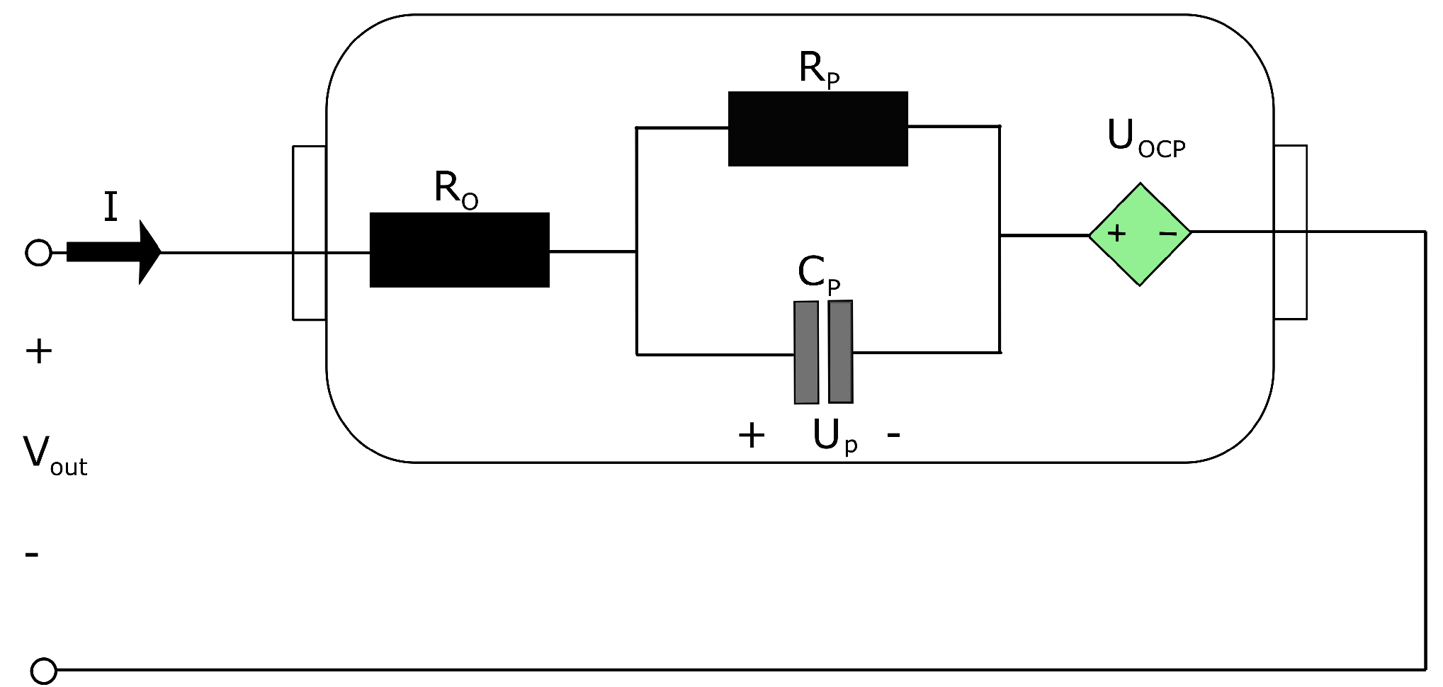
2.5. Improved Equivalent Circuit Model

From the numerical model, optimized parameters can be computed to create an ECM. Figure 2 shows the considered circuit. On the other hand, from the ROM, a continuous parameter estimation (CPE) or adaptation can be performed in order to improve the accuracy of the ECM.
In the simplest way, ECM uses Coulomb Counting CC 
d SOC d t ( t ) = I ( t ) Q max , t > 0 , SOC ( 0 ) = SOC 0 ,
with Q max denoting the maximum charge possible, and SOC 0 being an estimate of the initial SOC, to keep track of the SOC of the battery, or as in our model, of each electrode. Leaving aside the separated nature of two electrodes of different material and all related electrochemical processes and taking into account the inability of directly measuring the concentration distribution on the electrode surface, on the long run this approach requires a correction term as typically obtained from some state estimation technique.
Using the concentration of Li-ions obtained from the ROM, the ECM can be improved. As not all the data of x ¯ k is needed and just some part of it, the variable z k is defined in the following for the reduced model extraction. In addition, the voltage U p of the capacitor C p is converted to a discrete form.
z [ k ] = z 1 , [ k ] z 2 , [ k ] = C ¯ s C ¯ s + .
The variable ξ represents the states of the improved ECM model, i.e.,
ξ [ k ] = ξ 1 , [ k ] ξ 2 , [ k ] ξ 3 , [ k ] = U p z [ k ] ,
where in discrete time, e.g., using a simple Euler discretization with step Δ t the voltage U p is approximated by:
U p [ k ] = R p C p Δ t R p C p · U p [ k 1 ] + Δ t C p · I [ k 1 ] .
The tracking of the internal potential will use the improved ECM approach creating the following discrete-time system:
ξ [ k ] = A d ξ [ k 1 ] + B d u [ k 1 ]
V = h ( ξ , U ) = ξ 1 + U O C P + ( S O C + ) U O C P ( S O C ) + R o u 1
with
A d = R p C p Δ t R p C p 0 0 0 A ¯ C s 0 0 0 A ¯ C s + , B d = Δ t C p 0 B ¯ C s B ¯ C s +
S O C [ k ] + = U ^ C s + ( n , : ) · A ¯ C s + · ξ 3 , [ k ] · ( C s , m a x + ) 1
S O C [ k ] = U ^ C s ( n , : ) · A ¯ C s · ξ 2 , [ k ] · ( C s , m a x ) 1 .
In the system conformed by (36b) until (36e), ξ 1 , [ k ] is the RC sub-network voltage in discrete time, ξ 2 , [ k ] is the reduced state of the negative electrode concentration with the dimension r ^ 1 , and ξ 3 , [ k ] is the reduced state of the concentration of Lithium in the positive electrode with dimension r ^ 2 . The input u [ k ] is composed by the current and temperature. In (36d)–(36e) the original surface concentration of each electrode is recovered by using the state transformation U i ^ from (31). Note that the concentration profile over the complete electrode can be recovered, but as for the output voltage only the surface concentration is required, only the n t h columns of the state transformation matrices are used.

2.6. State Estimation

For the estimation process, a discrete version of the EKF with non-linear output function is considered [43,57]. This basically consists of the following steps:
(1) Prediction:
ξ ^ [ k ] = A d ξ ^ [ k 1 ] + B d u [ k 1 ] , ξ ^ [ 0 ] = ξ ^ 0
y ^ [ k ] = ξ ^ 1 , [ k ] + U O C P + ( S O C [ k ] + ) U O C P ( S O C [ k ] ) + R o · u 1 , [ k ]
P ^ [ k ] = A d P [ k 1 ] A d T + Q P [ 0 ] = P 0
(2) Kalman gain determination:
L [ k ] = P ^ [ k ] H [ k ] T R 1 , H [ k ] = h ( ξ , u ) ξ | ξ ^ [ k ] , u [ k ]
(3) Correction (innovation):
ξ ^ [ k ] = ξ ^ [ k ] + L [ k ] ( y [ k ] y ^ [ k ] )
As the functions U O C P ( S O C [ k ] ) are known, the partial derivatives of h ( ξ , u ) are easily calculated and can be used for the computation of the dynamic gain L [ k ] . R and Q are the covariance matrices of the measurement and process noise, respectively. For the initial values of the reduced stated of the concentration, the state transformation U i ^ from (31) is used
ξ ^ 2 , [ 0 ] = ( U ^ C s ) · S O C 0 · 1 ( C s , m a x )
ξ ^ 3 , [ 0 ] = ( U ^ C s + ) · S O C 0 + · 1 ( C s , m a x + )
where 1 represents a vector of ones of dimension n.

3. Evaluation Study

In this section the proposed method is evaluated using a comparison against a validated high-fidelity numerical model to identify (i) accuracy of the ROM and the ECM with continuous parameter estimation/adaptation (CPE) regarding the microscopic electrochemical states as well as the macroscopic electrical ones, and (ii) effectiveness with respect to computation times and memory requirements.

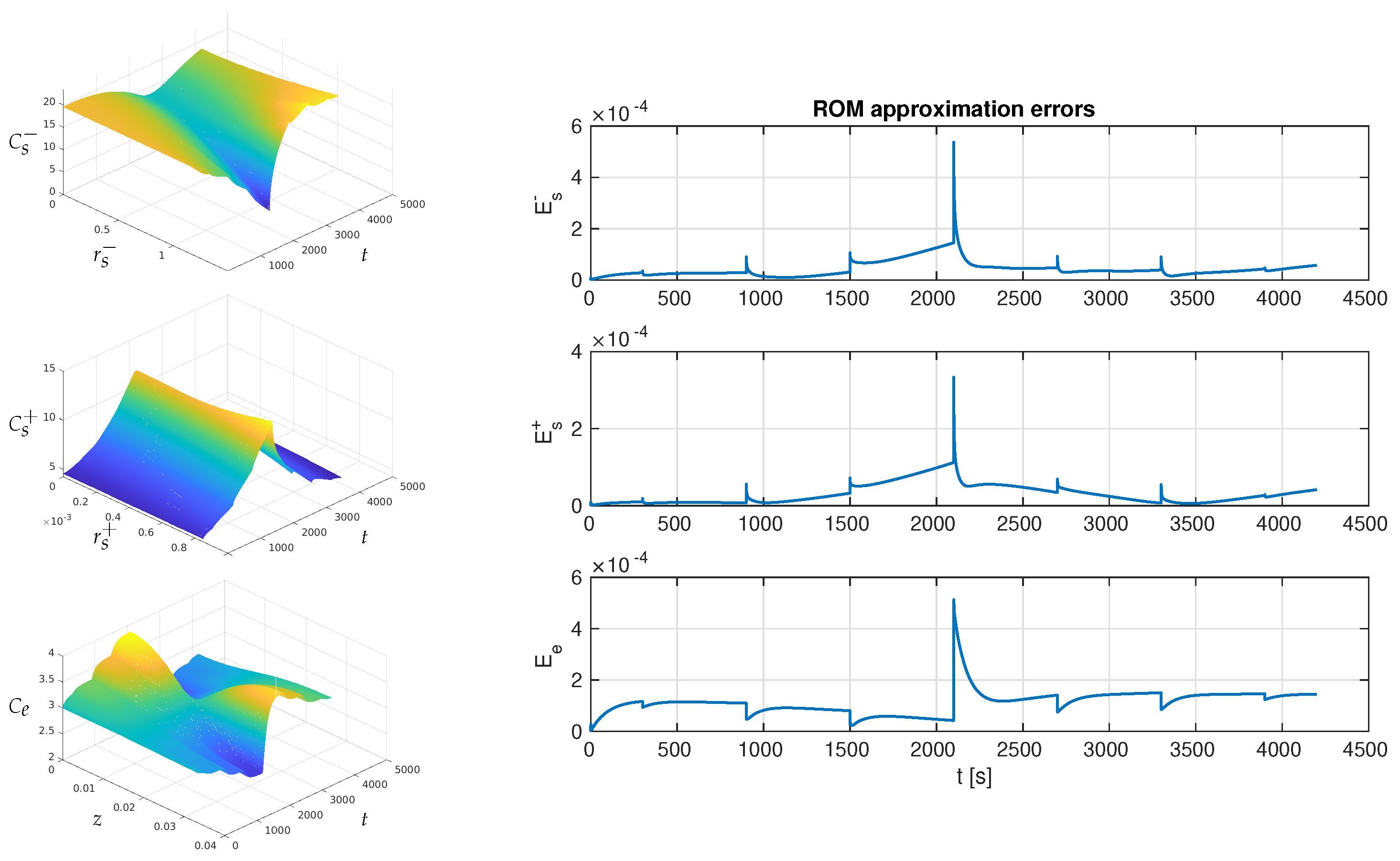
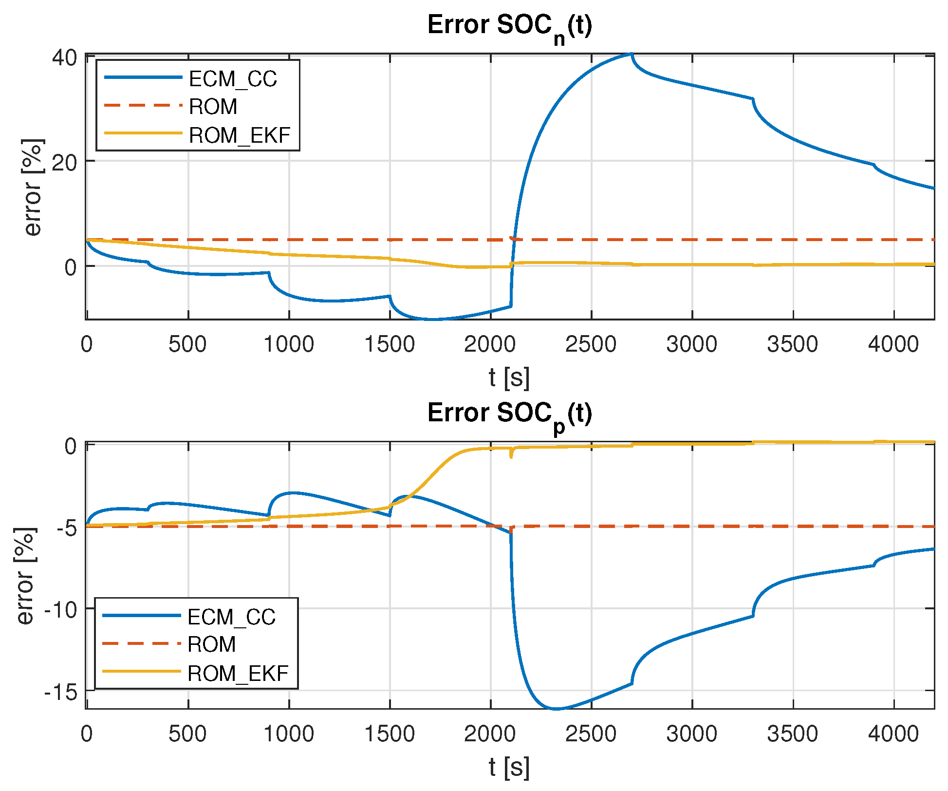
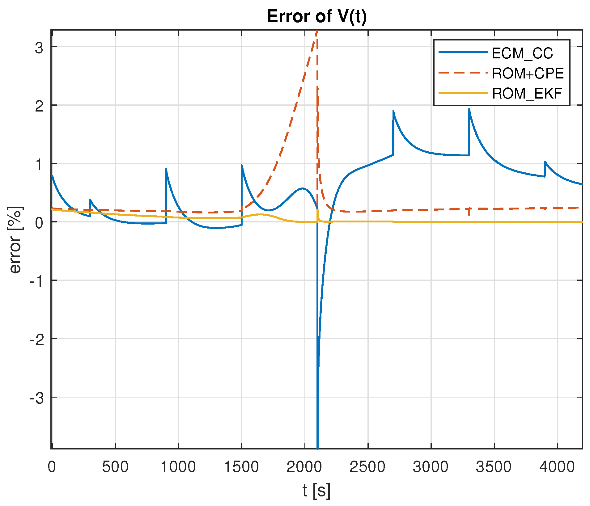
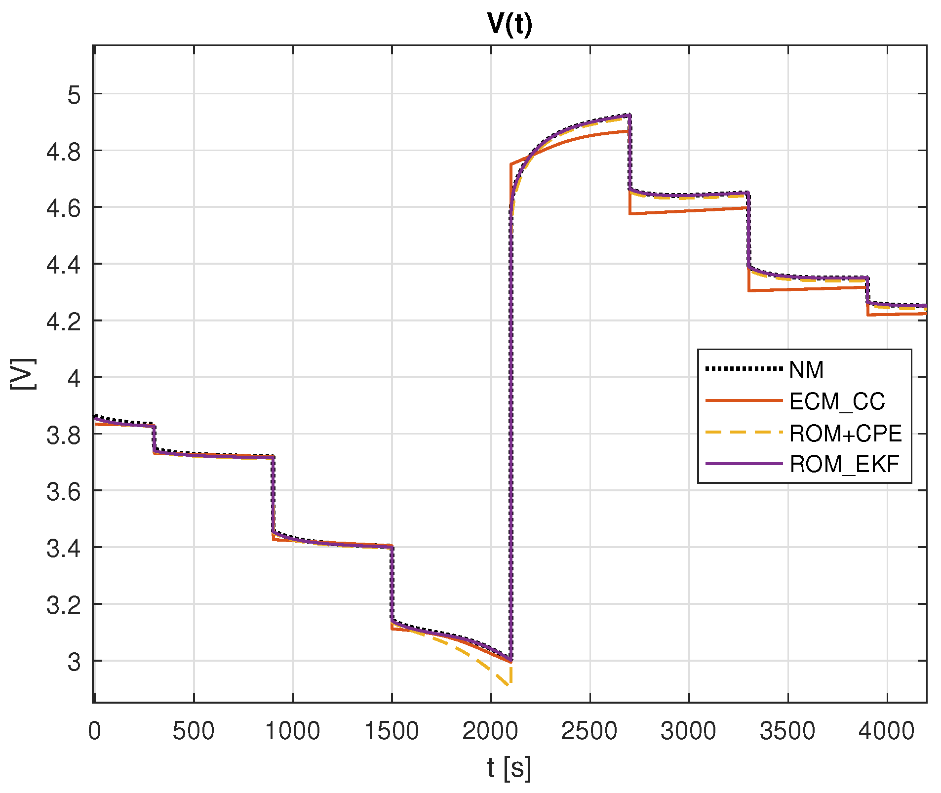
3.1. Numerical Evaluation

As commented in Section 2.3 the DMDc approach is repeated six times, one for each of the main variables of the electrochemical model using a time discretization step of Δ t = 0.5 s. More detail on the choice of training data can be found in [39]. Note that for the training scenarios with different charging and discharging scenarios and different temperatures were combined. The dimensions of the original system and the identified ROM are summarized in Table 1. The obtained dynamics matrix A ¯ has all eigenvalues within the unit circle, so that the identified system dynamics is input–output stable.
To test the accuracy and efficiency of the ROM with the improved ECMwith continuous parameter adaptation (CPE), and the combination with the EKF, as well as comparing these approaches against a simple constant parameter ECM with CC, a simulation was carried out for a 70 min discharge and charge process with the following C current rates: 1 3 C, 1 2 C, 1C, 1.5C, −1.5C, −1C, − 1 2 C, − 1 3 C with the external temperature being set to 30 °C. An initial error of 5% was considered for the values of the SOC of both electrodes at t = 0 . The values of the parameters for the numerical model simulation are provided in Appendix B.
The effectiveness of the ROM based on the considered DMDc identification procedure outlined above is evaluated first. Figure 3 shows the approximated profiles according to (28) for the concentrations of the electrodes (left column, top and center) and the electrolyte (left column, bottom), with the associated approximation errors (right column) in comparison to the high-fidelity numerical model. It can be clearly seen that the approximations are quite convincing inspite of the considerable order reduction according to Table 1. This illustrates clearly the strong approximation potential of the DMDc approach and its usefullness for the prediction of cell internal electrochemical states.
Figure 4 shows the error between the ROM, Coulomb counting (CC) and EKF and the numerical model for the surface SOC for both electrodes, which is derived from the Li-ion concentration. It can be seen that in comparison to an ECM with constant optimized parameters and simple CC, the ROM achieves a better prediction, which is further improved by the EKF, achieving a convergence over the simulation time, compensating the initial error.
Subsequently, Figure 5 shows the error of the output voltage V for the simulated discharge/charge process for the ECM with CC, ECM with continous parameter adaptation (CPE) based on the ROM and the ROM with the EKF, showing that the inclusion of the ECM by using the SOC predicted by the ROM according to (36) already achieves an improvement in comparison to the constant parameter ECM with CC, and that this is further improved significantly by coupling the ROM with the EKF. Figure 6 shows the associated output voltage. In both figures the superiority of the ROM-based approaches can be clearly seen in comparison to the ECM with CC using constant parameters and no correction terms, while a considerable additional further improvement is achieved with the ROM coupled to the EKF.
To have a one shot view of the performance of the ROM and its combination with the EKF, Table 2 and Table 3 show the root mean square error (RMSE) obtained in the simulations.

3.2. Discussion

As can be seen from the numerical evaluation study, the proposed approach is able to reconstruct microscopic electrochemical states (concentration and potential profiles) together with macroscopic electrical states (SOC, output voltage) in an efficient way, i.e., with low computational requirements and enabling potential real-time applications.
It should be noted that the data used for the identification of the ROM considered the cell temperature as an external signal, so the resulted model is capable to tackle changes on temperature making a good agreement for testing scenarios besides the standard 25°C. The ECM and CC with optimized parameters could not consider this effect, leading to a faster increasing discrepance to the actual states if the external temperature was shows deviations from the standard temperature.
The average root square error of the ROM is promising supporting the helpful use of the DMDc for complex systems that present a low-dimensional behaviour between sampling times. The RMSE for the concentration is less than 3 × 10 3 (lets recall that the SOC depends of the concentration on the solid phase) and for the terminal voltage is less than 100 μ V. In contrast, the standard equivalent circuit model (ECM) has a RMSE of around 40 mV for the terminal voltage. Additionally, the dimension of the ROM is only about 7% of the numerical model.
The processing time of the numerical model for the discharge/charge simulation study was of 75.9 s while the ROM only needed 1.6 s, i.e., around only 2% of the original time, enabling its potential future implementation in real-time applications.
It should be highlighted once more, that the ROM proceeds from equation free data, implying the resulted ROM depends only from the data produced during the numerical simulation of training data scenarios. Accordingly, different simulations would come up with slightly to considerably different truncation factors, dimensions and values for the ROM. Thus, it is important to define a priori what phenomena would be required to be reflected in the ROM and create an appropriate test scenario in terms of current and temperature.

4. Conclusions

An approach for effective estimation of the cell internal electrochemical states of a Li-ion battery based on DMDc was proposed. A systematic way of deriving the ROM was outlined starting with the single particle battery model, its numerical approximation using finite differences and the application of DMDc on each electrochemical state separately, given that this possibility is enabled by the system structure. In comparison to previous applications of DMDc for batteries the present study enables the consideration of electrochemical states and thermal dynamics. Based on the ROM an improved ECM was proposed for which the SOC is determined using the ROM instead of classical Coulomb counting (CC). The proposed ECM model was coupled with an EKF to enhance the model predictions by adequately combining them with output data from the battery. The approach was evaluated in numerical simulations for a validated high-fidelity model showing a high precision in the estimation of the microscopic electrochemical states as well as the macroscopic electrical states (SOC, output voltage), while keeping the numerical effort very low and thus enabling its potential implementation in real-time applications for monitoring and control purposes.

5. Future Work

The proposed DMDc modelling approach looks promising to achieve high prediction accuracy for the estimation of internal electrochemical states and thus in particular the associated SOC, overcoming the burden of computational complexity inherent to the numerical solution of detailed electrochemical models. As this paves the way for advanced feedback and optimal control design, different state-feedback control approaches should be studied and evaluated in particular for the governer design problem, optimal charging and cell balancing.
Further investigation is required to determine the inherent stability properties associated to the nonlinear interconnection introduced by the thermal dynamics and the approximation possiblities using DMDc and extended DMDc. Furthermore, the associated implications for state estimator and control design should be further analyzed.

Author Contributions

Conceptualization, H.M. and A.S., methodology, H.M. and A.S.; software, H.M.; validation, H.M.; formal analysis, H.M. and A.S.; investigation, H.M.; data curation, H.M.; writing—original draft preparation, H.M.; writing—review and editing, A.S.; visualization, H.M.; supervision, A.S. All authors have read and agreed to the published version of the manuscript.

Funding

This research received no external funding.

Informed Consent Statement

Not applicable.

Data Availability Statement

Not applicable.

Acknowledgments

H.M. gratefully acknowledges the scholarship from Erasmus Mundus in the framework of the Master Program E-PiCo, that has led to the oportunity of this study.

Conflicts of Interest

The authors declare no conflict of interest.

Abbreviations

The following abbreviations are used in this manuscript:
CPEContinuous parameter estimation/adaptation
DMDcDynamic Mode Decomposition with control
DMDDynamic Mode Decomposition
ECMEquivalent Circuit Model
EKFExtended Kalman Filter
I/OInput/Output
Li-ionLithium ions
ROMReduced Order Model
SOCState Of Charge
SVDSingular Value Decomposition

Appendix A. Matrices for the Finite-Difference Approximation

Using central differences and incorporating the boundary conditions one obtains the following matrices and vectors used in Section 2.2.
A C e = D e ( Δ x ) 2 1 1 0 0 0 0 1 2 1 0 0 0 0 0 0 1 2 1 0 0 0 0 1 1 , b C e = t e 0 F 1 δ 0 1 δ +
A Φ e = 1 0 0 0 0 0 0 0 0 1 0 0 0 0 0 0 1 0 1 0 0 0 0 0 0 0 0 0 1 0 1 0 0 0 0 0 0 1 0 1 b Φ e = 2 Δ x κ 0 0 0 0 0 0 0 1 δ 0 0 0 0 0 0 0 0 0 1 δ + 0 x T 2 Δ x κ 0 1 L δ + C Φ e = R T ( 1 t e 0 ) F 0 0 0 0 0 0 0 0 1 1 0 0 0 0 0 0 1 0 1 0 0 0 0 0 0 0 0 0 1 0 1 0 0 0 0 0 0 1 0 1
A C s = D s ( Δ r ) 2 1 1 0 0 0 0 0 1 2 1 0 0 0 0 0 0 0 0 1 2 1 0 0 0 0 0 1 1 + D s R s Δ r 1 1 0 0 0 0 0 0 1 0 1 0 0 0 0 0 0 1 0 1 0 0 0 0 0 0 0 0 0 1 0 1 0 0 0 0 0 0 1 1 b C s = Δ r + R s Δ r R s a s F δ 0 1

Appendix B. Modell Parameters

The parameters used in the simulation studies are listed in Table A1.
Table A1. Model parameters used in the simulation study.
ParameterValueDescription
D s [cm 2 /s] 3.9 × 10 9 Diffusion coefficient negative electrode
D s + [cm 2 /s] 1.0 × 10 9 Diffusion coefficient positive electrode
D e [cm 2 /s] 9.0 × 10 7 Diffusion coefficient electrolyte
C s , m a x [mol/dm 3 ]24.49Maximum concentration of negative electrode
C s , m a x + [mol/dm 3 ]22.86Maximum concentration of positive electrode
C e , m a x [mol/dm 3 ]20Maximum concentration of electrolyte
R s [ μ m]12.15Radius of negative electrode particle
R s + [ μ m]8.50Radius of positive electrode particle
ε 0.185Volume fraction
δ [S/cm]1Conductivity negative electrode
δ + [S/cm]0.038Conductivity positive electrode
κ [S/cm]2.8 × 10 4 Ionic conductivity of electrolyte
α 0.5Reaction rate
t e 0 0.2Transfer number of electrolyte
σ [ μ m]100Length of negative electrode
σ + [ μ m]174Length of positive electrode
σ s [ μ m]52Length of electrolyte
R f [ Ω ] 1000Film resistance negative electrode
R f + [ Ω ] 1200Film resistance positive electrode
r e f f 0.0122Rate constant anodic direct.
r e f f + 0.0058Rate constant cathodic direct.
T [K]298.15Temperature
F [A· /mol]96,485.3Faraday’s constant
R [J/mol · K]8.314Gas constant
1 C [mA· h/cm 2 ] 5.76C rate current
ρ a v g [Mg/m 2 ] 1.459Average mass per unit area
C p [J/Kg · K]2000Heat capacity
h 0 [W/m 2 · K]60Heat transfer coefficient

References

  1. Jossen, A. Fundamentals of battery dynamics. J. Power Sources 2006, 154, 530–538. [Google Scholar] [CrossRef]
  2. Valis, D.; Hasilova, K.; Leuchter, J. Modelling of influence of various operational conditions on Li-ion battery capability. In Proceedings of the 2016 IEEE International Conference on Industrial Engineering and Engineering Management (IEEM), Bali, Indonesia, 4–7 December 2016; pp. 536–540. [Google Scholar] [CrossRef]
  3. Ecker, M.; Shafiei Sabet, P.; Sauer, D.U. Influence of operational condition on lithium plating for commercial lithium-ion batteries—Electrochemical experiments and post-mortem-analysis. Appl. Energy 2017, 206, 934–946. [Google Scholar] [CrossRef]
  4. Zou, C.; Manzie, C.; Nešić, D. A Framework for Simplification of PDE-Based Lithium-Ion Battery Models. IEEE Trans. Control Syst. Technol. 2016, 24, 1594–1609. [Google Scholar] [CrossRef]
  5. Newman, J.; Tiedemann, W. Porous-electrode theory with battery applications. AIChE J. 1975, 21, 25–41. [Google Scholar] [CrossRef] [Green Version]
  6. Doyle, C. Design and Simulation of Lithium Rechargeable Batteries. Ph.D. Thesis, University of California, Lawrence Berkeley National Laboratory, Berkeley, CA, USA, 1995. [Google Scholar]
  7. Doyle, M.; Newman, J. The use of mathematical modeling in the design of lithium/polymer battery systems. Electrochim. Acta 1995, 40, 2191–2196. [Google Scholar] [CrossRef]
  8. Changfu, Z.; Manzie, C.; Nesic, D. PDE battery model simplification for charging strategy evaluation. In Proceedings of the 2015 10th Asian Control Conference (ASCC), Kinabalu, Malaysia, 31 May–3 June 2015; IEEE: Piscataway, NJ, USA, 2015; pp. 1–6. [Google Scholar]
  9. Doyle, M.; Fuller, T.F.; Newman, J. Modelling the Galvanostatic Charge and Discharge of the Lithium/Polymer/Insertion Cell. J. Electrochem. Soc. 1992, 140, 1526. [Google Scholar] [CrossRef]
  10. Kroener, C. A Mathematical Exploration of a PDE System for Lithium-Ion Batteries. Ph.D. Thesis, UC Berkeley, Berkeley, CA, USA, 2016. [Google Scholar]
  11. Perez, H.E. Model Based Optimal Control, Estimation, and Validation of Lithium-Ion Batteries. Ph.D. Thesis, UC Berkeley, Berkeley, CA, USA, 2016. [Google Scholar]
  12. Doyle, M.; Newman, J.; Gozdz, A.S.; Schmutz, C.N.; Tarascon, J.M. Comparison of Modeling Predictions with Experimental Data from Plastic Lithium Ion Cells. J. Electrochem. Soc. 1996, 143, 1890. [Google Scholar] [CrossRef]
  13. Thomas, K.E.; Newman, J.; Darling, R.M. Mathematical Modeling of Lithium Batteries. In Advances in Lithium-Ion Batteries; van Schalkwijk, W.A., Scrosati, B., Eds.; Springer: Boston, MA, USA, 2002; pp. 345–392. [Google Scholar]
  14. Klein, R.; Chaturvedi, N.A.; Christensen, J.; Ahmed, J.; Findeisen, R.; Kojic, A. State estimation of a reduced electrochemical model of a lithium-ion battery. In Proceedings of the 2010 American Control Conference, Baltimore, MD, USA, 30 June–2 July 2010; pp. 6618–6623. [Google Scholar]
  15. Klein, R.; Chaturvedi, N.A.; Christensen, J.; Ahmed, J.; Findeisen, R.; Kojic, A. Electrochemical model based observer design for a lithium-ion battery. IEEE Trans. Control Syst. Technol. 2012, 21, 289–301. [Google Scholar] [CrossRef]
  16. Tang, S.; Wang, Y.; Sahinoglu, Z.; Wada, T.; Hara, S.; Krstic, M. State-of-charge estimation for lithium-ion batteries via a coupled thermal-electrochemical model. In Proceedings of the 2015 American Control Conference (ACC), Chicago, IL, USA, 1–3 July 2015; pp. 5871–5877. [Google Scholar]
  17. Perez, H.; Shahmohammadhamedani, N.; Moura, S. Enhanced performance of li-ion batteries via modified reference governors and electrochemical models. IEEE/ASME Trans. Mechatronics 2015, 20, 1511–1520. [Google Scholar] [CrossRef]
  18. Perez, H.E.; Hu, X.; Moura, S.J. Optimal charging of batteries via a single particle model with electrolyte and thermal dynamics. In Proceedings of the 2016 American Control Conference (ACC), IEEE, Boston, MA, USA, 6–8 July 2016; pp. 4000–4005. [Google Scholar]
  19. Romagnoli, R.; Couto, L.D.; Kinnaert, M.; Garone, E. Control of the state-of-charge of a li-ion battery cell via reference governor. IFAC-PapersOnLine 2017, 50, 13747–13753. [Google Scholar] [CrossRef]
  20. Santhanagopalan, S.; Guo, Q.; Ramadass, P.; White, R.E. Review of models for predicting the cycling performance of lithium ion batteries. J. Power Sources 2006, 156, 620–628. [Google Scholar] [CrossRef]
  21. Zheng, F.; Xing, Y.; Jiang, J.; Sun, B.; Kim, J.; Pecht, M. Influence of different open circuit voltage tests on state of charge online estimation for lithium-ion batteries. Appl. Energy 2016, 183, 513–525. [Google Scholar] [CrossRef]
  22. Rausch, M.; Streif, S.; Pankiewitz, C.; Findeisen, R. Nonlinear observability and identifiability of single cells in battery packs. In Proceedings of the 2013 IEEE International Conference on Control Applications (CCA), Hyderabad, India, 28–30 August 2013; pp. 401–406. [Google Scholar]
  23. Chen, J.; Ouyang, Q.; Xu, C.; Su, H. Neural Network-Based State of Charge Observer Design for Lithium-Ion Batteries. IEEE Trans. Control Syst. Technol. 2018, 26, 313–320. [Google Scholar] [CrossRef]
  24. How, D.N.T.; Hannan, M.A.; Hossain Lipu, M.S.; Ker, P.J. State of Charge Estimation for Lithium-Ion Batteries Using Model-Based and Data-Driven Methods: A Review. IEEE Access 2019, 7, 136116–136136. [Google Scholar] [CrossRef]
  25. Di Domenico, D.; Fiengo, G.; Stefanopoulou, A. Lithium-ion battery state of charge estimation with a Kalman Filter based on a electrochemical model. In Proceedings of the 2008 IEEE International Conference on Control Applications, Antonio, TX, USA, 3–5 September 2008; pp. 702–707. [Google Scholar] [CrossRef] [Green Version]
  26. Di Domenico, D.; Stefanopoulou, A.; Fiengo, G. Lithium-Ion Battery State of Charge and Critical Surface Charge Estimation Using an Electrochemical Model-Based Extended Kalman Filter. J. Dyn. Syst. Meas. Control 2010, 132. [Google Scholar] [CrossRef]
  27. Smith, K.A.; Rahn, C.D.; Wang, C.Y. Control oriented 1D electrochemical model of lithium ion battery. Energy Convers. Manag. 2007, 48, 2565–2578. [Google Scholar] [CrossRef]
  28. Fan, G.; Canova, M. Model Order Reduction of Electrochemical Batteries Using Galerkin Method. In Proceedings of the Dynamic Systems and Control Conference, American Society of Mechanical Engineers (ASME), Columbus, OH, USA, 28–30 October 2015. [Google Scholar] [CrossRef]
  29. Fan, G.; Li, X.; Canova, M. A Reduced-Order Electrochemical Model of Li-Ion Batteries for Control and Estimation Applications. IEEE Trans. Veh. Technol. 2018, 67, 76–91. [Google Scholar] [CrossRef]
  30. Li, C.; Cui, N.; Wang, C.; Zhang, C. Reduced-order electrochemical model for lithium-ion battery with domain decomposition and polynomial approximation methods. Energy 2021, 221, 119662. [Google Scholar] [CrossRef]
  31. Li, Y.; Karunathilake, D.; Vilathgamuwa, D.M.; Mishra, Y.; Farrell, T.W.; Choi, S.S.; Zou, C. Model Order Reduction Techniques for Physics-Based Lithium-Ion Battery Management: A Survey. IEEE Ind. Electron. Mag. 2022, 16, 36–51. [Google Scholar] [CrossRef]
  32. Kutz, J.N.; Brunton, S.L.; Brunton, B.W.; Proctor, J.L. Dynamic Mode Decomposition: Data-Driven Modeling of Complex Systems; Society for Industrial and Applied Mathematics: Philadelphia, PA, USA, 2016. [Google Scholar]
  33. Tu, J.H.; Rowley, C.W.; Luchtenburg, D.M.; Brunton, S.L.; Kutz, J.N. On Dynamic Mode Decomposition: Theory and Applications. J. Comput. Dyn. 2014, 1, 391–421. [Google Scholar] [CrossRef] [Green Version]
  34. Proctor, J.L.; Brunton, S.L.; Kutz, J.N. Dynamic mode decomposition with control. arXiv 2014, arXiv:1409.6358. [Google Scholar] [CrossRef] [Green Version]
  35. Brunton, S.L.; Kutz, J.N. Data-Driven Science and Engineering: Machine Learning, Dynamical Systems, and Control; Cambridge University Press: Cambridge, UK, 2019. [Google Scholar]
  36. Lusch, B.; Kutz, J.N.; Brunton, S.L. Deep learning for universal linear embeddings of nonlinear dynamics. Nat. Commun. 2018, 9, 4950. [Google Scholar] [CrossRef] [PubMed] [Green Version]
  37. Baumann, H.; Schaum, A.; Meurer, T. Data-driven control-oriented reduced order modeling for open channel flows. IFAC-PapersOnLine 2022, 55, 193–199. [Google Scholar] [CrossRef]
  38. Abu-Seif, M.A.; Abdel-Khalik, A.S.; Hamad, M.S.; Hamdan, E.; Elmalhy, N.A. Data-Driven modeling for Li-ion battery using dynamic mode decomposition. Alex. Eng. J. 2022, 61, 11277–11290. [Google Scholar] [CrossRef]
  39. Moreno, H.; Schaum, A. Reduced-order electrochemical modelling of Lithium-ion batteries. In Proceedings of the 1st IFAC Workshop on Control of Complex Systems (COSY), Bologna, Italy, 24–25 November 2022; 2022. [Google Scholar]
  40. Luenberger, D. An introduction to observers. IEEE Trans. Autom. Control 1971, 16, 596–602. [Google Scholar] [CrossRef]
  41. Luenberger, D.G. Observing the State of a Linear System. IEEE Trans. Mil. Electron. 1964, 8, 74–80. [Google Scholar] [CrossRef]
  42. Zeitz, M. The extended Luenberger observer for nonlinear systems. Syst. Control Lett. 1987, 9, 149–156. [Google Scholar] [CrossRef]
  43. Jazwinski, A.H. Stochastic Processes and Filtering Theory; Academic Press: New York, NY, USA, 1970. [Google Scholar]
  44. Daum, F.E. Extended Kalman Filters. In Encyclopedia of Systems and Control; Baillieul, J., Samad, T., Eds.; Springer: London, UK, 2015; pp. 411–413. [Google Scholar]
  45. Lai, X.; Huang, Y.; Han, X.; Gu, H.; Zheng, Y. A novel method for state of energy estimation of lithium-ion batteries using particle filter and extended Kalman filter. J. Energy Storage 2021, 43, 103269. [Google Scholar] [CrossRef]
  46. Xiong, R.; Gong, X.; Mi, C.C.; Sun, F. A robust state-of-charge estimator for multiple types of lithium-ion batteries using adaptive extended Kalman filter. J. Power Sources 2013, 243, 805–816. [Google Scholar] [CrossRef]
  47. Rezoug, M.R.; Taibi, D.; Benaouadj, M. State-of-charge Estimation of Lithium-ion Batteries Using Extended Kalman Filter. In Proceedings of the 2021 10th International Conference on Power Science and Engineering (ICPSE), Istanbul, Turkey, 21–23 October 2021; pp. 98–103. [Google Scholar]
  48. Surana, A. Koopman Operator Based Observer Synthesis for Control-Affine Nonlinear Systems. In Proceedings of the IEEE 55th Conference on Decision and Control (CDC), Las Vegas, NV, USA, 12–14 December 2016; pp. 6492–6499. [Google Scholar]
  49. Surana, A.; Banaszuk, A. Linear observer synthesis for nonlinear systems using Koopman Operator framework. IFAC-PapersOnLine 2016, 49, 716–723. [Google Scholar] [CrossRef]
  50. Gomez, D.F.; Lagor, F.D.; Kirk, P.B.; Lind, A.H.; Jones, A.R.; Paley, D.A. Data-driven estimation of the unsteady flowfield near an actuated airfoil with embedded pressure sensors. J Guid. Control. Dyn. 2019, 42, 2279. [Google Scholar] [CrossRef]
  51. Vijayshankar, S.; Nabi, S.; Chakrabarty, A.; Grover, P.; Benosman, M. Dynamic Mode Decomposition and Robust Estimation: Case Study of a 2D Turbulent Boussinesq Flow. In Proceedings of the 2020 American Control Conference, Denver, CO, USA, 1–3 July 2020; pp. 2351–2356. [Google Scholar]
  52. Otto, S.E.; Rowley, C.W. Koopman Operators for Estimation and Control of Dynamical Systems. Annu. Rev. Control. Robot. Auton. Syst. 2021, 4, 59–87. [Google Scholar] [CrossRef]
  53. Schaum, A. Autoencoder-Based Reduced Order Observer Design for a Class of Diffusion-Convection-Reaction Systems. Algorithms 2021, 14, 330. [Google Scholar] [CrossRef]
  54. Fuller, T.F.; Doyle, M.; Newman, J. Simulation and Optimization of the Dual Lithium Ion Insertion Cell. J. Electrochem. Soc. 1994, 141, 1–10. [Google Scholar] [CrossRef]
  55. Aikens, D. Electrochemical Methods, Fundamentals and Applications; ACS Publications: Washington, DC, USA, 1983. [Google Scholar]
  56. Farlow, S. Partial Differential Equations for Scientists and Engineers; Dover books on advanced mathematics; Dover Publications: Mineola, NY, USA, 1993. [Google Scholar]
  57. Gelb, A. Applied Optimal Estimation; M.I.T. Press: Cambridge, MA, USA, 1978. [Google Scholar]
Figure 1. DUAL cell sandwich battery, cross-sectional view. The current collectors are located at the extremes of the cell, inspired by [54].
Algorithms 16 00073 g001
Figure 2. First Order RC Equivalent Circuit Model.
Algorithms 16 00073 g002
Figure 3. ROM approximation of concentration profiles (left column) for negative electrode (top), positive electrode (center) and electroylte (bottom), with the associated approximation error evolutions over time (right column).
Algorithms 16 00073 g003
Figure 4. Error for the Surface SOC of electrodes. S O C N M ( t 0 ) = [ 0.8 , 0.2 ] , S O C R ( t 0 ) = [ 0.75 , 0.25 ] , T = 30 °C and simulation time = 70 min.
Algorithms 16 00073 g004
Figure 5. Error of Output Potential V(t). S O C N M ( t 0 ) = [ 0.8 , 0.2 ] , S O C R ( t 0 ) = [ 0.75 , 0.25 ] , T = 30 °C and simulation time = 70 min.
Algorithms 16 00073 g005
Figure 6. Output Potential V(t). S O C N M ( t 0 ) = [ 0.8 , 0.2 ] , S O C R ( t 0 ) = [ 0.75 , 0.25 ] , T = 30 °C and simulation time = 70 min.
Algorithms 16 00073 g006
Table 1. DMDc approximation orders used for the model with parameters given in Appendix B.
Numerical ModelROM
C s 609
C s + 606
Φ s 602
Φ s + 602
C e 1304
Φ e 1309
total50032
Table 2. RMSE of the internal electrochemical states obtained by the DMDc based ROM with the EKF.
C s C s + Φ s Φ s + C e Φ e
RMSE2.8 × 10 3 2.7 × 10 3 1.8 × 10 8 2.3 × 10 6 5.8 × 10 4 5.4 × 10 2
Table 3. RMSE for the macroscopic output states for the ROM without and with the EKF.
SOC S SOC S + V(t)
ROM5.0 × 10 2 5.0 × 10 2 2.3 × 10 2
ROM+EKF1.9 × 10 2 2.8 × 10 2 2.9 × 10 3
Disclaimer/Publisher’s Note: The statements, opinions and data contained in all publications are solely those of the individual author(s) and contributor(s) and not of MDPI and/or the editor(s). MDPI and/or the editor(s) disclaim responsibility for any injury to people or property resulting from any ideas, methods, instructions or products referred to in the content.

