Improved Gradient Descent Iterations for Solving Systems of Nonlinear Equations

Abstract

This research proposes and investigates some improvements in gradient descent iterations that can be applied for solving system of nonlinear equations (SNE). In the available literature, such methods are termed improved gradient descent methods. We use verified advantages of various accelerated double direction and double step size gradient methods in solving single scalar equations. Our strategy is to control the speed of the convergence of gradient methods through the step size value defined using more parameters. As a result, efficient minimization schemes for solving SNE are introduced. Linear global convergence of the proposed iterative method is confirmed by theoretical analysis under standard assumptions. Numerical experiments confirm the significant computational efficiency of proposed methods compared to traditional gradient descent methods for solving SNE.

1. Introduction, Preliminaries, and Motivation

Our intention is to solve a system of nonlinear equations (SNE) of the general form

$$F\left(\mathbf{x}\right)=0,\mathbf{x}\in {\mathbb{R}}^n,$$

(1)

where $\mathbb{R}$ is the set of real numbers, ${\mathbb{R}}^n$ denotes the set of n-dimensional vectors from $\mathbb{R}$, and $F:{\mathbb{R}}^n\mapsto {\mathbb{R}}^n$, $F\left(\mathbf{x}\right)={(F_1\left(\mathbf{x}\right),\dots ,F_n\left(\mathbf{x}\right))}^{\mathrm{T}}$, and $F_i:{\mathbb{R}}^n\mapsto \mathbb{R}$ is the ith component of F. It is assumed that F is a continuously differentiable mapping. The nonlinear optimization problem (1) is equivalent to the subsequent minimization of the following goal function f:

$$\underset{\mathbf{x}\in {\mathbb{R}}^n}{min}f\left(\mathbf{x}\right),f\left(\mathbf{x}\right)=\frac{1}{2}{\parallel F\left(\mathbf{x}\right)\parallel }^2=\frac{1}{2}\sum _{i=1}^n{\left(F_i\left(\mathbf{x}\right)\right)}^2.$$

(2)

The equivalence of (1) and (2) is widely used in science and practical applications. In such problems, the solution to SNE (1) comes down to solving a related least-squares problem (2). In addition to that, the application of the adequate nonlinear optimization method in solving (1) is a common and efficient technique. Some well-known schemes for solving (1) are based on successive linearization, where the search direction ${\mathbf{d}}_k$ is obtained by solving the equation

$$F\left({\mathbf{x}}_k\right)+F^{\prime }\left({\mathbf{x}}_k\right){\mathbf{d}}_k=0,$$

(3)

where $F^{\prime }\left({\mathbf{x}}_k\right)\equiv J_F\left({\mathbf{x}}_k\right)$, and $J_F\left(\mathbf{x}\right)=\left[\frac{\partial F_1\left(\mathbf{x}\right)}{\partial {\mathbf{x}}_j}\right]$ is the Jacobian matrix of $F\left(\mathbf{x}\right)$. Therefore, the Newton iterative scheme for solving (1) is defined as

$${\mathbf{x}}_{k+1}={\mathbf{x}}_k+t_k{\mathbf{d}}_k={\mathbf{x}}_k-t_k{\left(F^{\prime }\left({\mathbf{x}}_k\right)\right)}^{-1}F\left({\mathbf{x}}_k\right),$$

(4)

where $t_k$ is a positive parameter that stands for the steplength value.

1.1. Overview of Methods for Solving SNE

Most popular iterations for solving (1) use appropriate approximations $B_k$ of the Jacobian matrix $F^{\prime }\left({\mathbf{x}}_k\right)$. These iterations are of the form ${\mathbf{x}}_{k+1}={\mathbf{x}}_k+t_k{\mathbf{d}}_k$, where $t_k$ is the steplength, and ${\mathbf{d}}_k$ is the search direction obtained as a solution to the SNE

$$B_k{\mathbf{d}}_k+F\left({\mathbf{x}}_k\right)=0.$$

(5)

For simplicity, we will use notations

$$F_k:=F\left({\mathbf{x}}_k\right),{\mathbf{y}}_k:=F_{k+1}-F_k,{\mathbf{s}}_k:={\mathbf{x}}_{k+1}-{\mathbf{x}}_k.$$

(6)

The BFGS approximations are defined on the basis of the secant equation $B_{k+1}{\mathbf{s}}_k={\mathbf{y}}_k$. The BFGS updates

$$B_{k+1}=B_k-\frac{B_k{\mathbf{s}}_k{\mathbf{s}}_k^{\mathrm{T}}{B}_k}{{\mathbf{s}}_k^{\mathrm{T}}{B}_k{\mathbf{s}}_k}+\frac{{\mathbf{y}}_k{\mathbf{y}}_k^{\mathrm{T}}}{{\mathbf{y}}_k^{\mathrm{T}}{\mathbf{s}}_k}$$

with an initial approximation $B_0\in {\mathbb{R}}^{n\times n}$ were considered in [1].

Further on, we list and briefly describe relevant minimization methods that exploit the equivalence between (1) and (2). The efficiency and applicability of these algorithms highly motivated the research presented in this paper. The number of methods that we mention below confirms the applicability of this direction in solving SNE. In addition, there is an evident need to develop and constantly upgrade the performances of optimization methods for solving (1).

There are numerous methods which can be used to solve the problem (1). Many of them are developed in [2,3,4,5,6,7]. Derivative-free methods for solving SNE were considered in [8,9,10]. These methods are proposed as appropriate adaptations of double direction and steplength methods in nonlinear optimization and the approximation of the Jacobian with a diagonal matrix whose entries are defined utilizing of an appropriate parameter. One approach based on various modifications of the Broyden method was proposed in [11,12]. A derivative-free conjugate gradient (CG) iterations for solving SNE were proposed in [13].

A descent Dai–Liao CG method for solving large-scale SNE was proposed in [14]. Novel hybrid and modified CG methods for finding a solution to SNE were originated in [15,16], respectively. An extension of a modified three-term CG method that can be applied for solving equations with convex constraints was presented in [17]. A diagonal quasi-Newton approach for solving large-scale nonlinear systems was considered in [18,19]. A quasi-Newton method, defined based on an improved diagonal Jacobian approximation, for solving nonlinear systems was proposed in [20]. Abdullah et al. in [21] proposed a double direction method for solving nonlinear equations. The first direction is the steepest descent direction, while the second direction is the proposed CG direction. Two derivative-free modifications of the CG-based method for solving large-scale systems $F\left(\mathbf{x}\right)=0$ were presented in [22]. These methods are applicable in the case when the Jacobian of $F\left(\mathbf{x}\right)$ is not accessible. An efficient approximation to the Jacobian matrix with a computational effort similar to that of matrix-free settings was proposed in [23]. Such efficiency was achieved when a diagonal matrix generates a Jacobian approximation. This method possesses low memory space requirements because the method is defined without computing exact gradient and Jacobian. Waziri et al. in [24] followed the approach based on the approximation of the Jacobian inverse by a nonsingular diagonal matrix. A fast and computationally efficient method concerning memory requirements was proposed in [25], and it uses an approximation of the Jacobian by an adequate diagonal matrix. A two-step generalized scheme of the Jacobian approximation was given in [26]. Further on, an iterative scheme which is based on a modification of the Dai–Liao CG method, classical Newton iterates, and the standard secant equation was suggested in [27]. A three-step method based on a proper diagonal updating was presented in [28]. A hybridization of FR and PRP conjugate gradient methods was given in [29]. The method in [29] can be considered as a convex combination of the PRP method and the FR method while using the hyperplane projection technique. A diagonal Jacobian method was derived from data from two preceding steps, and a weak secant equation was investigated in [30]. An iterative modified Newton scheme based on diagonal updating was proposed in [31]. Solving nonlinear monotone operator equations via a modified symmetric rank-one update is given in [32]. In [33], the authors used a new approach in solving nonlinear systems by simply considering them in the form of multi-objective optimization problems.

It is essential to mention that the analogous idea of avoiding the second derivative in the classical Newton’s method for solving nonlinear equations is exploited in deriving several iterative methods of various orders for solving nonlinear equations [34,35,36,37]. Moreover, some derivative-free iterative methods were developed for solving nonlinear equations [38,39]. Furthermore, some alternative approaches were conducted for solving complex symmetric linear systems [40] or a Sylvester matrix equation [41].

Trust region methods have become very popular algorithms for solving nonlinear equations and general nonlinear problems [37,42,43,44].

The systems of nonlinear equations (1) have various applications [15,29,45,46,47,48], for example in solving the ${\ell }_1$-norm problem arising from compressing sensing [49,50,51,52], in variational inequalities problems [53,54], and optimal power flow equations [55] among others.

Viewed statistically, the Newton method and different forms of quasi-Newton methods have been frequently used in solving SNE. Unfortunately, methods of the Newton family are not efficient in solving large-scale SNE problems since they are based on the Jacobian matrix. A similar drawback applies to all methods based on various matrix approximations of the Jacobian matrix in each iteration. Numerous adaptations and improvements of the CG iterative class exist as one solution applicable to large-scale problems. We intend to use the simplest Jacobian approximation using an appropriate diagonal matrix. Our goal is to define computationally effective methods for solving large-scale SNEs using the simplest of Jacobian approximations. The realistic basis for our expectations is the known efficient methods used to optimize individual nonlinear functions.

The remaining sections have the following general structure. The introduction, preliminaries, and motivation are included in Section 1. An overview of methods for solving SNE is presented in Section 1.1 to complete the presentation and explain the motivation. The motivation for the current study is described in Section 1.2. Section 2 proposes several multiple-step-size methods for solving nonlinear equations. Convergence analysis of the proposed methods is investigated in Section 3. Section 4 contains several numerical examples obtained on main standard test problems of various dimensions.

1.2. Motivation

The following standard designations will be used. We adopt the standard notations for the gradient $\mathbf{g}\left(\mathbf{x}\right):=\nabla f\left(\mathbf{x}\right)$ and the Hessian $G\left(\mathbf{x}\right):={\nabla }^{2}f\left(\mathbf{x}\right)$ of the objective function $f\left(\mathbf{x}\right)$. Further, ${\mathbf{g}}_k=\mathbf{g}\left({\mathbf{x}}_k\right)$ denotes the gradient vector for f in the point ${\mathbf{x}}_k$. An appropriate identity matrix will be denoted by I.

Our research is motivated by two trends in solving minimization problems. These streams are described as two subsequent parts of the current subsection. A nonlinear multivariate unconstrained minimization problem is defined as

$$minf\left(\mathbf{x}\right),\mathbf{x}\in {\mathbb{R}}^n,$$

(7)

where $f\left(\mathbf{x}\right):{\mathbb{R}}^n\mapsto \mathbb{R}$ is a uniformly convex or strictly convex continuously differentiable function bounded from below.

1.2.1. Improved Gradient Descent Methods as Motivation

The most general iteration for solving (7) is expressed as

$${\mathbf{x}}_{k+1}={\mathbf{x}}_k+t_k{\mathbf{d}}_k.$$

(8)

In (8), ${\mathbf{x}}_{k+1}$ presents a new approximation point based on the previous ${\mathbf{x}}_k$. Positive parameter $t_k$ stays for the steplength value, while ${\mathbf{d}}_k$ presents the search direction vector, which is generated based on the descent condition

$${\mathbf{g}}_k^{\mathrm{T}}{\mathbf{d}}_k<0.$$

The direction vector ${\mathbf{d}}_k$ may be defined in various ways. This vital element is often determined using the features of the function gradient. In one of the earliest optimization schemes, the gradient descent method (GD), this variable is defined as negative of the gradient direction, i.e., ${\mathbf{d}}_k=-{\mathbf{g}}_k$. In the line search variant of the Newton method, the search direction presents the solution to the system of nonlinear equations $G_k\mathbf{d}=-{\mathbf{g}}_k$ with respect to $\mathbf{d}$, where $G_k:=G({\mathbf{x}}_k)={▽}^{2}f\left({\mathbf{x}}_k\right)$ denotes the Hessian matrix.

Unlike traditional GD algorithms for nonlinear unconstrained minimization, which are defined based on a single step size $t_k$, a class of improved gradient descent ($IGD$) algorithms define the final step size using two or more steps size scaling parameters. Such algorithms were classified and investigated in [56]. Obtained numerical results confirm that the usage of appropriate additional scaling parameters decreases the number of iterations. Typically, one of the parameters is defined using the inexact line search, while the second one is defined using the first terms of the Taylor expansion of the goal function.

A frequently investigated class of minimization methods that can be applied for solving the problem (7) use the following iterative rule

$${\mathbf{x}}_{k+1}={\mathbf{x}}_k-{\theta }_k{t}_k{\mathbf{g}}_k.$$

(9)

In (9), the parameter $t_k$ represents the step size in the kth iteration. The originality of the iteration (9) is expressed though the acceleration variable ${\theta }_k$. This type of optimization scheme with acceleration parameter was originated in [57]. Later, in [58], the authors justifiably named such models as accelerated gradient descent methods (AGD methods shortly). Further research on this topic confirmed that the acceleration parameter generally improves the performance of the gradient method.

The Newton method with included line search technique is defined by the following iterative rule

$${\mathbf{x}}_{k+1}={\mathbf{x}}_k-t_k{G}_k^{-1}{\mathbf{g}}_k,$$

(10)

wherein $G_k^{-1}$ stands for the inverse of the Hessian matrix $G_k$. Let $B_k$ be a symmetric positive definite matrix such that $\parallel B_k-G_k\parallel <ϵ$, for arbitrary matrix norm $\parallel .\parallel$ and for a given tolerance $ϵ$. Further, let $H_k$ be a positive definite approximation of the Hessian’s inverse $G_k^{-1}$. This approach leads to the relation (11) which is the quasi-Newton method with line search:

$${\mathbf{x}}_{k+1}={\mathbf{x}}_k-t_k{H}_k{\mathbf{g}}_k.$$

(11)

Updates of $H_k$ can be defined as solutions to the quasi-Newton equation

$$H_{k+1}{\mathbf{y}}_k={\mathbf{s}}_k,$$

(12)

where ${\mathbf{s}}_k={\mathbf{x}}_{k+1}-{\mathbf{x}}_k$, ${\mathbf{y}}_k={\mathbf{g}}_{k+1}-{\mathbf{g}}_k$. There is a class of iterations (11) in which there is no ultimate requirement for the $H_k$ to satisfy the quasi-Newton equation. Such a class of iterates is known as modified Newton methods [59].

The idea in [58] is usage of a proper diagonal approximation of the Hessian

$$B_k={\gamma }_{k}I,{\gamma }_k>0,{\gamma }_k\in \mathbb{R}.$$

(13)

Applying the approximation (13) of $B_k$, the matrix $H_k$ can be approximated by the simple scalar matrix

$$H_k={\gamma }_k^{-1}I.$$

(14)

In this way, the quasi-Newton line search scheme (11) is transformed into a kind of $AGD$ iteration, called the $SM$ method and presented in [58] as

$${\mathbf{x}}_{k+1}={\mathbf{x}}_k-{\gamma }_k^{-1}{t}_k{\mathbf{g}}_k.$$

(15)

The positive quantity ${\gamma }_k$ is the convergence acceleration parameter which improves the behavior of the generated iterative loop. In [56], methods of the form (15) are termed as improved gradient descent methods (IGD). Commonly, the primary step size $t_k$ is calculated through the features of some inexact line search algorithms. An additional acceleration parameter ${\gamma }_k$ is usually determined by the Taylor expansion of the goal function. This way of generating acceleration parameter is confirmed as a good choice in [56,58,60,61,62].

The choice ${\gamma }_k:=1$ in the $IGD$ iterations (15) reveal the $GD$ iterations

$${\mathbf{x}}_{k+1}={\mathbf{x}}_k-t_k{\mathbf{g}}_k.$$

(16)

On the other hand, if the acceleration ${\gamma }_k$ is well-defined, then the step size $t_k:=1$ in the $IGD$ iterations (15) is acceptable in most cases [63], which leads to a kind of the $GD$ iterative principle:

$${\mathbf{x}}_{k+1}={\mathbf{x}}_k-{\gamma }_k^{-1}{\mathbf{g}}_k.$$

(17)

Barzilai and Borwein in [64] proposed two efficient $IGD$ variants, known as $BB$ method variants, where the steplength ${\gamma }_k^{BB}$ was defined as an approximation $H_k={\gamma }_k^{BB}I$. Therefore, the replacement ${\gamma }_k^{-1}:={\gamma }_k^{BB}$ in (17) leads to the $BB$ iterative rule

$${\mathbf{x}}_{k+1}={\mathbf{x}}_k-{\gamma }_k^{BB}{\mathbf{g}}_k.$$

The scaling parameter ${\gamma }_k^{BB}$ in the basic version is defined upon the minimization of the vector norm $\underset{\gamma }{min}{\parallel {\mathbf{s}}_{k-1}-\gamma {\mathbf{y}}_{k-1}\parallel }^2$, which gives

$${\gamma }_k^{BB}=\frac{{\mathbf{s}}_{k-1}^{\mathrm{T}}{\mathbf{y}}_{k-1}}{{\mathbf{y}}_{k-1}^{\mathrm{T}}{\mathbf{y}}_{k-1}}.$$

(18)

The steplength ${\gamma }_k^{BB}$ in the dual method is produced by the minimization $\underset{\gamma }{min}{\parallel \gamma {\mathbf{s}}_{k-1}-{\mathbf{y}}_{k-1}\parallel }^2$, which yields

$${\gamma }_k^{BB}=\frac{{\mathbf{s}}_{k-1}^{\mathrm{T}}{\mathbf{s}}_{k-1}}{{\mathbf{s}}_{k-1}^{\mathrm{T}}{\mathbf{y}}_{k-1}}.$$

(19)

The $BB$ iterations were modified and investigated in a number of publications [65,66,67,68,69,70,71,72,73,74,75,76,77,78,79]. The so-called Scalar Correction ($SC$) method from [80] proposed the trial steplength in (17) defined by

$${\gamma }_{k+1}^{SC}=\left\{\begin{array}{cc}\frac{{\mathbf{s}}_k^{\mathrm{T}}{\mathbf{r}}_k}{{\mathbf{y}}_k^{\mathrm{T}}{\mathbf{r}}_k},\hfill & {\mathbf{y}}_k^{\mathrm{T}}{\mathbf{r}}_k>0\hfill \\ \frac{\parallel {\mathbf{s}}_k\parallel }{\parallel {\mathbf{y}}_k\parallel },\hfill & {\mathbf{y}}_k^{\mathrm{T}}{\mathbf{r}}_k\le 0\hfill \end{array}\right.,{\mathbf{r}}_k={\mathbf{s}}_k-{\gamma }_k{\mathbf{y}}_k.$$

(20)

The $SC$ iterations are defined as

$${\mathbf{x}}_{k+1}={\mathbf{x}}_k-{\gamma }_k^{SC}{\mathbf{g}}_k.$$

A kind of steepest descent and $BB$ iterations relaxed by a parameter ${\theta }_k\in (0,2)$ were proposed in [81]. The so-called Relaxed Gradient Descent Quasi Newton methods, (shortly $RGDQN$ and $RGDQN1$), expressed by

$${\mathbf{x}}_{k+1}={\mathbf{x}}_k-{\theta }_k{t}_k{\gamma }_k^{-1}{\mathbf{g}}_k,$$

(21)

are introduced in [82]. Here, ${\theta }_k$ presents the relaxation parameter. This value is chosen randomly within the $(0,1)$ interval in the $RGDQN$ schemes and by the relation

$${\theta }_k=\frac{{\gamma }_k}{t_k{\gamma }_{k+1}}$$

in the $RGDQN1$ algorithm.

1.2.2. Discretization of Gradient Neural Networks (GNN) as Motivation

Our second motivation arises from discretizing gradient neural network (GNN) design. A GNN evolution can be defined in three steps. Further details can be found in [83,84].

The bulleted lists look like this:

Step1GNN. 

Define underlying error matrix $E\left(t\right)$ by the interchange of the unknown matrix in the actual problem by the unknown time-varying matrix $V\left(t\right)$, which will be approximated over time $t\ge 0$. The scalar objective of a GNN is just the Frobenius norm of $E\left(t\right)$:

$$\epsilon \left(t\right)=\frac{{\parallel E\left(t\right)\parallel }_F^2}{2},{\parallel E\parallel }_F=\sqrt{\mathrm{Tr}\left(E^{\mathrm{T}}E\right)}.$$

Step2GNN. 

Compute the gradient $\frac{\partial \epsilon \left(t\right)}{\partial V}=\nabla \epsilon \left(t\right)$ of the objective $\epsilon \left(t\right)$.

Step3GNN. 

Apply the dynamic GNN evolution, which relates the time derivative $\dot{V}\left(t\right)$ and direction opposite to the gradient of $\epsilon \left(t\right)$:

$$\dot{V}\left(t\right)=\frac{\mathrm{d}V\left(t\right)}{\mathrm{d}t}=-\gamma \frac{\partial \epsilon \left(t\right)}{\partial V},V\left(0\right)=V_0.$$

(22)

Here, $V\left(t\right)$ is the activation state variables matrix, $t\in [0,+\infty )$ is the time, $\gamma >0$ is the gain parameter, and $\dot{V}\left(t\right)$ is the time derivative of $V\left(t\right)$.

The discretization of $\dot{V}\left(t\right)$ by the Euler forward-difference rule is given by

$$\dot{V}\left(t\right)\approx (V_{k+1}-V_k)/\tau ,$$

(23)

where $\tau$ is the sampling time and $V_k=V(t=k\tau )$, $k=1,2,\dots$ [84]. The approximation (23) transforms the continuous-time GNN evolution (23) into discrete-time iterations

$$\frac{V_{k+1}-V_k}{\tau }=-\gamma \frac{\partial \epsilon \left(t\right)}{\partial V}=-\gamma \nabla \epsilon \left(t\right).$$

Derived discretization of the GNN design is just a GD method for nonlinear optimization:

$$V_{k+1}=V_k-{\beta }_k\nabla \epsilon \left(t\right),{\beta }_k=\tau \gamma >0,$$

(24)

where ${\beta }_k=\tau \gamma >0$ is the step size. So, the step size ${\beta }_k$ is defined as a product of two parameters, in which the parameter $\gamma$ should be “as large as possible”, while $\tau$ should be “as small as possible”. Such considerations may add additional points of view to multiple parameters gradient optimization methods.

Our idea is to generalize the IGD iterations considered in [56] to the problem of solving SNE. One observable analogy is that the gain parameter $\gamma$ from (22) corresponds to the parameter ${\gamma }_k$ from (15). In addition, the sampling time $\tau$ can be considered as an analogy to the primary step size $t_k\in (0,1)$, which is defined by an inexact line search. Iterations defined as IGD iterations adopted to solve SNE will be called IGDN class.

2. Multiple Step-Size Methods for Solving SNE

The term “multiple step-size methods” is related to the class of gradient-based iterative methods for solving SNE employing a step size defined using two or more appropriately defined parameters. The final goal is to improve the efficiency of classical gradient methods. Two strategies are used in finding approximate parameters: inexact line search and the Taylor expansion.

2.1. IGDN Methods for Solving SNE

Our aim is to simplify the update of the Jacobian $F^{\prime }\left({\mathbf{x}}_k\right):=J_k$. Following (13), it is appropriate to approximate the Jacobian with a diagonal matrix

$$F^{\prime }\left({\mathbf{x}}_k\right)\approx {\gamma }_{k}I.$$

(25)

Then, $B_k={\gamma }_{k}I$ in (5) produces the search direction ${\mathbf{d}}_k=-{\gamma }_k^{-1}{F}_k$, and the iterations (8) are transformed into

$${\mathbf{x}}_{k+1}={\mathbf{x}}_k-t_k{\gamma }_k^{-1}{F}_k.$$

(26)

The final step size in iterations (26) is defined using two step size parameters: $t_k$ and ${\gamma }_k$. Iterations that fulfill pattern (26) are an analogy of $IGD$ methods for nonlinear unconstrained optimization and will be termed as $IGDN$ class of methods.

Using the experience of nonlinear optimization, the steplength parameter ${\gamma }_k$ can be defined appropriately using the Taylor expansion of $F\left(\mathbf{x}\right)$:

$$F_{k+1}=F_k+F^{\prime }\left({\xi }_k\right)\left({\mathbf{x}}_{k+1}-{\mathbf{x}}_k\right),{\xi }_k\in [{\mathbf{x}}_k,{\mathbf{x}}_{k+1}]$$

On the basis of (25), it is appropriate to use $F^{\prime }\left({\xi }_k\right)\approx {\gamma }_{k}I$, which implies

$$F_{k+1}-F_k={\gamma }_k\left({\mathbf{x}}_{k+1}-{\mathbf{x}}_k\right).$$

(27)

Using (27) and applying notation (6), one obtains the following updates of ${\gamma }_k$:

$${\gamma }_k=\frac{{\mathbf{y}}_k^{\mathrm{T}}{\mathbf{y}}_k}{{\mathbf{y}}_k^{\mathrm{T}}{\mathbf{s}}_k}=\frac{{\mathbf{s}}_k^{\mathrm{T}}{\mathbf{y}}_k}{{\mathbf{s}}_k^{\mathrm{T}}{\mathbf{s}}_k}.$$

It can be noticed that the iterative rule (26) matches with $BB$ iteration [64]. So, we introduced the $BB$ method for solving SNE. Our further contribution is the introduction of appropriate restrictions on the scaling parameter. To that end, Theorem 1 reveals values of ${\gamma }_k$ which decrease the objective functions included in $F_k$. The inequality $F_{k+1}\le F_k$ means ${\left(F_{k+1}\right)}_i\le {\left(F_k\right)}_i$, $i=1,\dots ,n$.

Theorem 1.

If the condition ${\gamma }_{k+1}\le \frac{{\gamma }_k}{t_k}$ is satisfied, then the $IGDN$ iterations (26) satisfy $F_{k+1}\le F_k.$

Proof. 

As a consequence of (26) and (27), one can verify

$$F_{k+1}=F_k-t_k{\gamma }_{k+1}{\gamma }_k^{-1}{F}_k=\left(1-t_k{\gamma }_{k+1}{\gamma }_k^{-1}\right)F_k.$$

(28)

In view of $t_k,{\gamma }_{k+1},{\gamma }_k\ge 0$, it follows that $1-t_k{\gamma }_{k+1}{\gamma }_k^{-1}\le 1$. On the other hand, the inequality $1-t_k{\gamma }_{k+1}{\gamma }_k^{-1}\ge 0$ is satisfied in the case ${\gamma }_{k+1}\le \frac{{\gamma }_k}{t_k}$. Now, (28) implies ${\left(F_{k+1}\right)}_i\le {\left(F_k\right)}_i$, $i=1,\dots ,n$, which needs to be proven.    □

So, appropriate update ${\gamma }_{k+1}$ can be defined as follows:

$${\gamma }_{k+1}=\left\{\begin{array}{cc}\frac{{\mathbf{y}}_k^{\mathrm{T}}{\mathbf{y}}_k}{{\mathbf{y}}_k^{\mathrm{T}}{\mathbf{s}}_k}=\frac{{\mathbf{s}}_k^{\mathrm{T}}{\mathbf{y}}_k}{{\mathbf{s}}_k^{\mathrm{T}}{\mathbf{s}}_k},\hfill & {\mathbf{y}}_k^{\mathrm{T}}{\mathbf{s}}_k\ge 0,\hfill \\ \frac{{\gamma }_k}{t_k},\hfill & {\mathbf{y}}_k^{\mathrm{T}}{\mathbf{s}}_k<0.\hfill \end{array}\right.$$

(29)

Now, we are able to generate the value of the next approximation in the form

$${\mathbf{x}}_{k+2}={\mathbf{x}}_{k+1}-t_{k+1}{\gamma }_{k+1}^{-1}{F}_{k+1}.$$

(30)

The step size $t_{k+1}$ in (30) can be determined using the nonmonotone line search. More precisely, $t_k$ is defined by $t_k=max\left\{1,s^k\right\}$, where $s\in (0,1)$, and the integer k is defined from the line search

$$f({\mathbf{x}}_k+t_k{\mathbf{d}}_k)-f\left({\mathbf{x}}_k\right)\le -{\omega }_1\left|\right|t_{k}F\left({\mathbf{x}}_k\right){\left|\right|}^2-{\omega }_2\left|\right|t_k{\mathbf{d}}_k{\left|\right|}^2+{\eta }_{k}f\left({\mathbf{x}}_k\right),$$

(31)

wherein ${\omega }_1>0$, ${\omega }_2>0$, are constants, and $\left\{{\eta }_k\right\}$ is a positive sequence such that

$$\sum _{k=0}^{\infty }{\eta }_k<\infty .$$

(32)

The equality (28) can be rewritten in the equivalent form

$${\mathbf{y}}_k=-t_k{\gamma }_{k+1}{\gamma }_k^{-1}{F}_k,$$

(33)

which gives

$${\gamma }_{k+1}=-\frac{{\gamma }_k{F}_k^{\mathrm{T}}{\mathbf{y}}_k}{t_k{F}_k^{\mathrm{T}}{F}_k}.$$

Further, an application of Theorem 1 gives the following additional update for the acceleration parameter ${\gamma }_k$:

$${\gamma }_{k+1}=\left\{\begin{array}{cc}-\frac{{\gamma }_k{F}_k^{\mathrm{T}}{\mathbf{y}}_k}{t_k{F}_k^{\mathrm{T}}{F}_k},\hfill & \frac{F_k^{\mathrm{T}}{\mathbf{y}}_k}{F_k^{\mathrm{T}}{F}_k}\notin (-1,0),\hfill \\ \frac{{\gamma }_k}{t_k},\hfill & \frac{F_k^{\mathrm{T}}{\mathbf{y}}_k}{F_k^{\mathrm{T}}{F}_k}\in (-1,0).\hfill \end{array}\right.$$

(34)

Corollary 1.

$IGDN$ iterations (26) determined by (34) satisfy $F_{k+1}\le F_k.$

Proof. 

Clearly, (34) initiates ${\gamma }_{k+1}\le \frac{{\gamma }_k}{t_k}$, and the proof follows from Theorem 1.    □

Further on, the implementation framework of the $IGDN$ method is presented in Algorithm 1.

Algorithm 1 The IGDN iterations based on  (29),  (30) or (34), (30).

Require:  Vector function $F\left(\mathbf{x}\right)$, $ϵ>0$ and initialization ${\mathbf{x}}_0\in {\mathbb{R}}^n$. 1: For $k=0$ chose ${\gamma }_0=1$ and $F\left({\mathbf{x}}_0\right)$. 2: Check the output criterion; if $∥F\left({\mathbf{x}}_k\right)∥\le ϵ$ is fulfilled then stop the algorithm; else, continue performing the next step. 3: (Line search) Compute $t_k\in (0,1]$ using (31). 4: Compute ${\mathbf{x}}_{k+1}$ using (30). 5: Determine ${\gamma }_{k+1}$ using (29) or (34). 6: $k:=k+1$. 7: Return to Step 2. 8: Outputs: ${\mathbf{x}}_{k+1}$, $F\left({\mathbf{x}}_{k+1}\right)$.

Remark 1.

The IGDN algorithm defined by (29) (resp. by (34)) will be denoted by $IGDN$ (29) (resp. by $IGDN$(34)). Mathematically, $IGDN$(29) and $IGDN$ (34) are equivalent. The numerical comparison of these algorithms will be performed later.

2.2. A Class of Accelerated Double Direction (ADDN) Methods

In [61], an optimization method was defined by the iterative rule

$${\mathbf{x}}_{k+1}={\mathbf{x}}_k+t_k{\mathbf{d}}_k+t_k^2{\mathbf{c}}_k,$$

(35)

where $t_k$ denotes the value of the steplength parameter, and ${\mathbf{d}}_k$, ${\mathbf{c}}_k$ are the search directions vectors. The vector ${\mathbf{d}}_k$ is defined as in the SM-method from [58], which gives ${\mathbf{d}}_k={{\gamma }_k}^{-1}{\mathbf{g}}_k$, and further

$${\mathbf{x}}_{k+1}={\mathbf{x}}_k-t_k{{\gamma }_k}^{-1}{\mathbf{g}}_k+t_k^2{\mathbf{c}}_k.$$

(36)

We want to apply this strategy in solving (1). First of all, the vector ${\mathbf{c}}_k$ can be defined according to [85]. An appropriate definition of ${\mathbf{c}}_k$ is still open.

Assuming again $B_k={\gamma }_{k}I$, the vector ${\mathbf{d}}_k$ from (5) becomes ${\mathbf{d}}_k=-{\gamma }_k^{-1}{F}_k$, which transforms (35) into

$${\mathbf{x}}_{k+1}={\mathbf{x}}_k-t_k{\gamma }_k^{-1}{F}_k+t_k^2{\mathbf{c}}_k.$$

(37)

We propose the steplength ${\gamma }_{k+1}$ arising from the Taylor expansion (27) and defined as in (29). In addition, it is possible to use an alternative approach. More precisely, in this case, (27) yields to

$$F_{k+1}=F_k-{\gamma }_{k+1}\left(-t_k{\gamma }_k^{-1}{F}_k+t_k^2{\mathbf{c}}_k\right).$$

As a consequence, ${\gamma }_{k+1}$ can be defined utilizing

$${\gamma }_{k+1}=-\frac{{\gamma }_k{\mathbf{y}}_k^{\mathrm{T}}{\mathbf{y}}_{\mathbf{k}}}{{\mathbf{y}}_k^{\mathrm{T}}\left(-t_k{F}_k+{\gamma }_k{t}_k^2{\mathbf{c}}_k\right)}.$$

(38)

The problem ${\gamma }_{k+1}<0$ in (38) is solved using ${\gamma }_{k+1}=1$.

We can easily conclude that the next iteration is then generated by

$${\mathbf{x}}_{k+2}={\mathbf{x}}_{k+1}-t_{k+1}{F}_{k+1}+t_k^2{\mathbf{c}}_{k+1}.$$

The $ADDN$ iterations are defined in Algorithm 2.

Algorithm 2 The $ADDN$ iterations based on (37), (38).

Require:  Functions $F\left(\mathbf{x}\right)$, $ϵ>0$ and a given initial vector ${\mathbf{x}}_0\in {\mathbb{R}}^n$. 1: For $k=0$ chose ${\gamma }_0=1$ and $F\left({\mathbf{x}}_0\right)$. 2: Check the stop criterion; if $∥F\left({\mathbf{x}}_k\right)∥\le ϵ$ is satisfied then stop the algorithm; else, continue with Step 3:. 3: (Line search) Find $t_k\in (0,1]$ using inexact line search procedure. 4: Compute ${\mathbf{x}}_{k+1}$ using (37). 5: Determine ${\gamma }_{k+1}$ using (38). 6: In case ${\gamma }_{k+1}<0$, apply ${\gamma }_{k+1}=1$. 7: $k:=k+1$. 8: Back to Step 2. 9: Outputs: ${\mathbf{x}}_{k+1}$, $F\left({\mathbf{x}}_{k+1}\right)$.

2.3. A Class of Accelerated Double Step Size (ADSSN) Methods

If the steplength $t_k^2$ is replaced by another steplength $l_k$ in (35), it can be obtained

$${\mathbf{x}}_{k+1}={\mathbf{x}}_k+t_k{\mathbf{d}}_k+l_k{\mathbf{c}}_k.$$

(39)

Here, the parameters $t_k,l_k\ge 0$ are two independent step size values, and the vectors ${\mathbf{d}}_k$, ${\mathbf{c}}_k$ define the search directions of the proposed iterative scheme (39).

Motivation for this type of iterations arises from [60]. The author of this paper suggested a model of the form (39) with two-step size parameters. This method is actually defined by substituting the parameter ${t_k}^2$ from (35) with another step size parameter $l_k$. Both step size values are computed by independent inexact line search algorithms.

Since we aim to unify search directions, it is possible to use

$${\mathbf{d}}_k:=-{\gamma }_k^{-1}{F}_k,{\mathbf{c}}_k:=-F_k.$$

(40)

The substitution of chosen parameters (40) into (39) produces

$${\mathbf{x}}_{k+1}={\mathbf{x}}_k-\left(t_k{\gamma }_k^{-1}+l_k\right)F_k.$$

(41)

The final step size, $\left(t_k{\gamma }_k^{-1}+l_k\right)$, in the iterations (41) are defined combining three step size parameters: $t_k$, $l_k$, and ${\gamma }_k$. Again, the parameter ${\gamma }_{k+1}$ is defined using the Taylor series of the form

$$F\left({\mathbf{x}}_{k+1}\right)=F\left({\mathbf{x}}_k\right)-{\gamma }_{k+1}\left(t_k{\gamma }_k^{-1}+l_k\right)F\left({\mathbf{x}}_k\right).$$

As a consequence, ${\gamma }_{k+1}$ can be computed by

$${\gamma }_{k+1}=-\frac{{\gamma }_k{F}_k^{\mathrm{T}}{\mathbf{y}}_{\mathbf{k}}}{(t_k+{\gamma }_k{l}_k)F_k^{\mathrm{T}}{F}_k}.$$

Theorem 2.

If the condition ${\gamma }_{k+1}\le \frac{{\gamma }_k}{t_k+{\gamma }_k{l}_k}$ holds, then the iterations (41) satisfy $F_{k+1}\le F_k.$

Proof. 

Taking (27) in conjunction with (41), one can verify

$$F_{k+1}=F_k-{\gamma }_{k+1}\left(t_k{\gamma }_k^{-1}+l_k\right)F_k=F_k\left(1-{\gamma }_{k+1}\left(t_k{\gamma }_k^{-1}+l_k\right)\right).$$

Clearly, ${\gamma }_{k+1}\le \frac{{\gamma }_k}{t_k+{\gamma }_k{l}_k}$ implies $1-{\gamma }_{k+1}\left(t_k{\gamma }_k^{-1}+l_k\right)\ge 0$. The proof follows from $t_k\ge 0,{\gamma }_{k+1},{\gamma }_k\ge 0$, which ensures $1-{\gamma }_{k+1}\left(t_k{\gamma }_k^{-1}+l_k\right)\le 1$.    □

In view of Theorem 2, it is reasonable to define the following update for ${\gamma }_{k+1}$ in the $ADSSN$ method:

$${\gamma }_{k+1}=\left\{\begin{array}{cc}-\frac{{\gamma }_k{F}_k^{\mathrm{T}}{\mathbf{y}}_{\mathbf{k}}}{(t_k+{\gamma }_k{l}_k)F_k^{\mathrm{T}}{F}_k},\hfill & \frac{F_k^{\mathrm{T}}{\mathbf{y}}_k}{F_k^{\mathrm{T}}{F}_k}\notin (-1,0),\hfill \\ \frac{{\gamma }_k}{t_k+{\gamma }_k{l}_k},\hfill & \frac{F_k^{\mathrm{T}}{\mathbf{y}}_k}{F_k^{\mathrm{T}}{F}_k}\in (-1,0).\hfill \end{array}\right.$$

(42)

Once the accelerated parameter ${\gamma }_{k+1}>0$ is determined, the values of step size parameters $t_{k+1}$ and $l_{k+1}$ are defined. Then, it is possible to generate the next point:

$$F_{k+2}=F_{k+1}-{\gamma }_{k+2}\left(t_{k+1}{\gamma }_{k+1}^{-1}+l_{k+1}\right)F_{k+1}.$$

In order to derive appropriate values of the parameters $t_{k+1}$ and $l_{k+1}$, we investigate the function

$${\Phi }_{k+1}(t,l)=F_{k+1}-{\gamma }_{k+2}\left({\gamma }_{k+1}^{-1}t+l\right)F_{k+1}.$$

The gradient of ${\Phi }_{k+1}(t,l)$ is equal to

$$\mathbf{g}\left({\Phi }_{k+1}(t,l)\right)=\left\{{\Phi }_{k+1}{(t,l)}_t^{\prime },{\Phi }_{k+1}{(t,l)}_l^{\prime }\right\}=\left\{-{\gamma }_{k+2}{\gamma }_{k+1}^{-1}{F}_{k+1},-{\gamma }_{k+2}{F}_{k+1}\right\}.$$

(43)

Therefore,

$${\Phi }_{k+1}(0,0)=F_{k+1}.$$

In addition,

$$\mathbf{g}\left({\Phi }_{k+1}(t,l)\right)=\{0,0\}⟺F_{k+1}=0.$$

(44)

Therefore, the function ${\Phi }_{k+1}(t,l)$ is well-defined.

Step scaling parameters $t_k$ and $l_k$ can be determined using two successive line search procedures (31).

Corollary 2.

The $ADSSN$ iterations determined by (41) satisfy $F_{k+1}\le F_k.$

Proof. 

Clearly, the definition of ${\gamma }_{k+1}$ in (42) implies ${\gamma }_{k+1}\le \frac{{\gamma }_k}{t_k}$, and the proof follows from Theorem 2.    □

The $ADSSN$ iterations are defined in Algorithm 3.

Algorithm 3 The $ADSSN$ iteration based on (41) and (42).

Require:  Chosen $F\left(\mathbf{x}\right)$, $ϵ>0$ and an initialization ${\mathbf{x}}_0\in {\mathbb{R}}^n$. 1: For $k=0$ chose ${\gamma }_0=1$ and $F\left({\mathbf{x}}_0\right)$. 2: Check the test criterion; if $∥F\left({\mathbf{x}}_k\right)∥\le ϵ$ holds, then stop; else, continue with Step 3:. 3: Find $t_k$ using inexact line search. 4: Find $l_k$ using inexact line search. 5: Compute ${\mathbf{x}}_{k+1}$ using (41). 6: Determine the scalar ${\gamma }_{k+1}$ using (42). 7: $k:=k+1$. 8: Return to Step 2:. 9: Outputs: ${\mathbf{x}}_{k+1}$ and $F\left({\mathbf{x}}_{k+1}\right)$.

Remark 2.

Step 6 of Algorithm 3 is defined according to Theorem 2.

2.4. Simplified ADSSN

Applying the relation

$$t_k+l_k=1$$

(45)

between the step size parameters $t_k$ and $l_k$ in the $ADSSN$ iterative rule (41), the $ADSSN$ iteration is transformed to

$${\mathbf{x}}_{k+1}={\mathbf{x}}_k-\left[t_k({\gamma }_k^{-1}-1)+1\right]F\left({\mathbf{x}}_k\right).$$

(46)

The convex combination (45) of step size parameters $t_k$ and $l_k$ that appear in the $ADSSN$ scheme (41) was originally proposed in [62] and applied in an iterative method for solving the unconstrained optimization problem (7). The assumption (45) represents a trade-off between the steplength parameters $t_k$ and $l_k$. In [62], it was shown that the induced single step size method shows better performance characteristics in general. The constraint (45) initiates the reduction of the two-parameter $ADSSN$ rule into a single step size transformed $ADSSN$ (shortly $TADSSN$) iterative method (46).

We can spot that the $TADSSN$ method is a modified version of $IGDN$ iterations, based on the replacement of the product $t_k{\gamma }_k^{-1}$, from the classical IGDN iteration, by the multiplying factor $t_k({\gamma }_k^{-1}-1)+1$.

The substitution ${\varphi }_k:=t_k({\gamma }_k^{-1}-1)+1$ will be used to simplify the presentation. Here, the accelerated parameter value ${\gamma }_{k+1}$ is calculated by (29).

Corollary 3.

Iterations (46) satisfy

$$F_{k+1}=F_k-{\gamma }_{k+1}{\varphi }_k{F}_k.$$

(47)

Proof. 

It follows from (27) and (46).    □

In view of (47), it is possible to conclude

$${\gamma }_{k+1}=-\frac{F_k^{\mathrm{T}}{\mathbf{y}}_{\mathbf{k}}}{{\varphi }_k{F}_k^{\mathrm{T}}{F}_k}.$$

Corollary 4 gives some useful restrictions on this rule.

Corollary 4.

If the condition ${\gamma }_{k+1}\le \frac{{\gamma }_k}{t_k+{\gamma }_k(1-t_k)}$ holds, then the iterations (41) satisfy $F_{k+1}\le F_k.$

Proof. 

It follows from Theorem 1 and $l_k=1-t_k$.    □

In view of Corollary 4, it is reasonable to define the following update for ${\gamma }_{k+1}$ in the $TADSSN$ method:

$${\gamma }_{k+1}=\left\{\begin{array}{cc}-\frac{F_k^{\mathrm{T}}{\mathbf{y}}_{\mathbf{k}}}{{\varphi }_k{F}_k^{\mathrm{T}}{F}_k},\hfill & \frac{F_k^{\mathrm{T}}{\mathbf{y}}_{\mathbf{k}}}{{\varphi }_k{F}_k^{\mathrm{T}}{F}_k}\le 0\hfill \\ \frac{{\gamma }_k}{t_k+{\gamma }_k(1-t_k)},\hfill & \frac{F_k^{\mathrm{T}}{\mathbf{y}}_{\mathbf{k}}}{{\varphi }_k{F}_k^{\mathrm{T}}{F}_k}>0.\hfill \end{array}\right.$$

(48)

Then, ${\mathbf{x}}_{k+2}$ is equal to

$${\mathbf{x}}_{k+2}={\mathbf{x}}_{k+1}-{\varphi }_{k+1}{F}_{k+1}.$$

Algorithm 4 The ADSSN iteration based on (46) and (48).

Require:  Chosen $F\left(\mathbf{x}\right)$, $ϵ>0$ and ${\mathbf{x}}_0\in {\mathbb{R}}^n$. 1: For $k=0$ chose ${\gamma }_0=1$ and $F\left({\mathbf{x}}_0\right)$. 2: Check the termination criterion; if $∥F\left({\mathbf{x}}_k\right)∥\le ϵ$ holds then stop; else, go to Step 3:. 3: (Line search) Apply (31) and generate the step size value $t_k$. 4: Compute $l_k=1-t_k$. 5: Compute ${\mathbf{x}}_{k+1}$ using (46). 6: Determine the scaling factor ${\gamma }_{k+1}$ using (48). 7: $k:=k+1$. 8: Return to Step 2. 9: Output: ${\mathbf{x}}_{k+1}$, $F\left({\mathbf{x}}_{k+1}\right)$.

3. Convergence Analysis

The level set is defined as

$$\Omega =\left\{\mathbf{x}\in {\mathbb{R}}^n|∥F\left(\mathbf{x}\right)∥\le ∥F\left({\mathbf{x}}_0\right)∥\right\},$$

(49)

where ${\mathbf{x}}_0\in {\mathbb{R}}^n$ is an initial approximation.

Therewith, the next assumptions are needed:

$\left(A_1\right)$

The level set $\Omega$ defined in (49) is bounded below.

$\left(A_2\right)$

Lipschitz continuity holds for the vector function F, i.e., $∥F\left(\mathbf{x}\right)-F\left(\mathbf{y}\right)∥\le r∥\mathbf{x}-\mathbf{y}∥$ for all $\mathbf{x},\mathbf{y}\in {\mathbb{R}}^n$ and $r>0$.

$\left(A_3\right)$

The Jacobian $F^{\prime }\left(\mathbf{x}\right)$ is bounded.

Lemma 1.

Suppose the assumption $\left(A_2\right)$ holds. If the sequence $\left\{{\mathbf{x}}_k\right\}$ is obtained by the $IGDN$ (29) iterations, then

$${\mathbf{y}}_k^{\mathrm{T}}{\mathbf{s}}_k\le r{∥{\mathbf{s}}_k∥}^2,r>0.$$

(50)

Proof. 

Obviously,

$${\mathbf{y}}_k^{\mathrm{T}}{\mathbf{s}}_k={\mathbf{s}}_k^{\mathrm{T}}{\mathbf{y}}_k={\mathbf{s}}_k^{\mathrm{T}}\left(F_{k+1}-F_k\right).$$

(51)

Therefore, assuming $\left(A_2\right)$, it is possible to derive

$${\mathbf{y}}_k^{\mathrm{T}}{\mathbf{s}}_k\le ∥{\mathbf{s}}_k∥∥F_{k+1}-F_k∥\le r{∥{\mathbf{s}}_k∥}^2.$$

(52)

Previous estimation confirms that (50) is satisfied with r defined by the Lipschitz condition in $\left(A_2\right)$. □

For the convergence results of the remaining algorithms, we need to prove the finiteness of ${\gamma }_k$, ${\mathbf{d}}_k$, and the remaining results follow trivially.

Lemma 2.

The ${\gamma }_k$ generated by $IGDN$ (29) is bounded by the Lipschitz constant r.

Proof. 

Clearly, the complemental step size ${\gamma }_k$ defined by (29) satisfies

$${\gamma }_{k+1}=\frac{{\mathbf{y}}_k^{\mathrm{T}}{\mathbf{s}}_k}{{∥{\mathbf{s}}_k∥}^2}\le \frac{r{∥{\mathbf{s}}_k∥}^2}{{∥{\mathbf{s}}_k∥}^2}=r,$$

(53)

which leads to the conclusion ${\gamma }_k\le r$. □

Lemma 3.

The additional step size ${\gamma }_k$ generated by $IGDN$ (34) is bounded as follows:

$${\gamma }_k\le \frac{1}{{\displaystyle \prod _{i=0}^{k-1}}{t}_i}$$

(54)

Proof. 

The updating rule (34) satisfies ${\gamma }_{k+1}\le \frac{{\gamma }_k}{t_k}$. Continuing in the same way, one concludes

$${\gamma }_{k+1}\le \frac{{\gamma }_0}{{\displaystyle \prod _{i=0}^k}{t}_i}.$$

The proof can be finished using ${\gamma }_0=1$. □

Lemma 4.

The additional scaling parameter ${\gamma }_k$ generated by (42) is bounded as follows:

$${\gamma }_k\le \frac{1}{{\displaystyle \prod _{i=0}^{k-1}}(t_i+{\gamma }_i{l}_i)}.$$

(55)

Lemma 5.

The directions ${\mathbf{d}}_k$ used in $IGDN$ (29) and $IGDN$ (34) algorithms are descent directions.

Proof. 

Since

$${\mathbf{d}}_k=-{\gamma }_k^{-1}{F}_k,$$

(56)

an application of the scalar product of both sides in (56) with $F_k^{\mathrm{T}}$ in conjunction with Lemma 2 leads to the following conclusion for $IGDN$ (29) iterations:

$$F_k^{\mathrm{T}}{\mathbf{d}}_k=-{\gamma }_k^{-1}{F}_k^{\mathrm{T}}{F}_k\le -\frac{1}{r}{∥F_k∥}^2<0.$$

(57)

With Lemma 3, it can be concluded that $IGDN$ (34) iterations imply the following:

$$F_k^{\mathrm{T}}{\mathbf{d}}_k=-{\gamma }_k^{-1}{F}_k^{\mathrm{T}}{F}_k\le -\left({\displaystyle \prod _{i=0}^{k-1}}{t}_i\right){∥F_k∥}^2<0.$$

(58)

The proof is complete. □

Lemma 6.

The direction ${\mathbf{d}}_k$ used in $ADSSN$ algorithms is a descent direction.

Proof. 

Since

$${\mathbf{d}}_k=-\left(t_k{\gamma }_k^{-1}+l_k\right)F_k,$$

(59)

after using the scalar product of both sides in (59) with $F_k^{\mathrm{T}}$ and taking into account Lemma 4, we obtain

$$\begin{array}{cc}{F}_k^{\mathrm{T}}{\mathbf{d}}_k\hfill & =-\left(t_k{\gamma }_k^{-1}+l_k\right)F_k^{\mathrm{T}}{F}_k\hfill \\ & =-\frac{1}{{\gamma }_k}\left(t_k+l_k{\gamma }_k\right)F_k^{\mathrm{T}}{F}_k\hfill \\ & \le -\frac{1}{\frac{1}{{\displaystyle \prod _{i=0}^{k-1}}(t_i+{\gamma }_i{l}_i)}}\left(t_k+l_k{\gamma }_k\right)F_k^{\mathrm{T}}{F}_k\hfill \\ & =-\left({\displaystyle \prod _{i=0}^k}(t_i+{\gamma }_i{l}_i)\right){∥F_k∥}^2<0.\hfill \end{array}$$

(60)

The proof is complete. □

Theorem 3.

The vector $F_{k+1}$ generated by $IGDN$ (34) is a descent direction.

Proof. 

According to (34), it follows

$${\gamma }_{k+1}=-\frac{{\gamma }_k{F}_k^{\mathrm{T}}{\mathbf{y}}_k}{t_k{F}_k^{\mathrm{T}}{F}_k}=-\frac{{\gamma }_k{F}_k^{\mathrm{T}}\left(F_{k+1}-F_k\right)}{t_k{F}_k^{\mathrm{T}}{F}_k}=-\frac{{\gamma }_k{F}_k^{\mathrm{T}}{F}_{k+1}}{t_k{\parallel F_k\parallel }^2}+\frac{{\gamma }_k}{t_k}.$$

As a consequence, ${\gamma }_{k+1}\le \frac{{\gamma }_k}{t_k}$ implies $F_k^{\mathrm{T}}{F}_{k+1}\ge 0$, which means that $F_{k+1}$ is a descent direction. □

Theorem 4.

The vector $F_{k+1}$ generated by $ADSSN$ iterations (41) is a descent direction.

Lemma 7.

If the assumptions $\left(A_1\right)$ and $\left(A_2\right)$ are valid, then the norm of the direction vector ${\mathbf{d}}_k$ generated by $IGDN$ (29) is bounded.

Proof. 

The norm $∥{\mathbf{d}}_k∥$ can be estimated as

$$\begin{array}{cc}∥{\mathbf{d}}_k∥\hfill & =∥-{\gamma }_k^{-1}{F}_k∥\hfill \\ & \le \left|-{\gamma }_k^{-1}\right|∥F_k∥.\hfill \end{array}$$

(61)

As an implication of $\left(A_1\right)$, one can conclude $∥F_k∥\le M$, which in conjunction with Lemma 2 further approximates $∥{\mathbf{d}}_k∥$ in (61) by $∥{\mathbf{d}}_k∥\le w$, $w=\frac{1}{r}M>0.$ □

Lemma 8.

If the assumptions $\left(A_1\right)$ and $\left(A_2\right)$ hold, then the norm of the direction vector ${\mathbf{d}}_k$ generated by $IGDN$ (34) is bounded.

Proof. 

As an implication of $\left(A_1\right)$, one can conclude $∥F_k∥\le M$, which in conjunction with (54) and (61) further approximates $∥{\mathbf{d}}_k∥$ in (61) by $∥{\mathbf{d}}_k∥\le w$, $w=\left({\displaystyle \prod _{i=0}^{k-1}}{t}_i\right)M>0.$ □

Lemma 9.

If the assumptions $\left(A_1\right)$ and $\left(A_2\right)$ are active, then the norm of the direction vector ${\mathbf{d}}_k$ generated by $ADSSN$ is bounded.

Proof. 

Following the proof used in Lemma 8, it can be verified that

$∥{\mathbf{d}}_k∥\le \left({\displaystyle \prod _{i=0}^{k-1}}\left(t_i{\gamma }_i^{-1}+l_i\right)\right)M>0.$□

Now, we are going to establish the global convergence of $IGDN$ (29) and $IGDN$ (34) and $ADSSN$ iterations.

Theorem 5.

If the assumptions $\left(A_2\right)$ and $\left(A_3\right)$ are satisfied and ${\mathbf{x}}_k$ are iterations generated by $IGDN$ (29), then

$$\underset{k\to \infty }{lim}∥F\left({\mathbf{x}}_k\right)∥=0.$$

(62)

Proof. 

The search direction is defined by ${\mathbf{d}}_k=-{\gamma }_k^{-1}{F}_k.$ Starting from the apparent relation

$$F_k^{\mathrm{T}}{\mathbf{d}}_k=-{\gamma }_k^{-1}{∥F_k∥}^2,$$

we can conclude

$${∥F_k∥}^2=-F_k^{\mathrm{T}}{\mathbf{d}}_k{\gamma }_k.$$

(63)

Finally, (57) implies $F_k^{\mathrm{T}}{\mathbf{d}}_k<0$, which further implies $-F_k^{\mathrm{T}}{\mathbf{d}}_k>0$. From Lemma 2, using (63) and $-F_k^{\mathrm{T}}{\mathbf{d}}_k>0$, it follows that

$$\begin{array}{cc}{∥F_k∥}^2\hfill & ={\gamma }_k|-F_k^{\mathrm{T}}{\mathbf{d}}_k|\hfill \\ & \le r\left|F_k^{\mathrm{T}}{\mathbf{d}}_k\right|\hfill \\ & \le r\parallel F_k\parallel \parallel {\mathbf{d}}_k\parallel .\hfill \end{array}$$

(64)

Based on Lemma 7, it can be concluded

$${∥F_k∥}^2\le r\parallel F_k\parallel \parallel {\mathbf{d}}_k\parallel \le rw\parallel F_k\parallel .$$

(65)

By Lemma 5, we can deduce that the norm of the function $F\left({\mathbf{x}}_k\right)$ is decreasing along the direction ${\mathbf{d}}_k$, which means $∥F\left({\mathbf{x}}_{k+1}\right)∥\le ∥F\left({\mathbf{x}}_k\right)∥$ is true for every k. Based on this fact, it follows

$$0\le {∥F_k∥}^2\le rw\parallel F_k\parallel ⟶0,$$

(66)

which directly implies

$$\underset{k\to \infty }{lim}∥F\left({\mathbf{x}}_k\right)∥=0$$

(67)

and completes the proof. □

Theorem 6.

If the assumptions $\left(A_2\right)$ and $\left(A_3\right)$ are satisfied and ${\mathbf{x}}_k$ are iterations generated by $IGDN$ (34), then (62) is valid.

Proof. 

The search direction of $IGDN$ (34) satisfies (63). Finally, since ${\gamma }_k$ is bounded as in (54), and ${\mathbf{d}}_k$ is a descent direction (Lemma 8). iIt can be concluded

$$\begin{array}{cc}0\le {∥F_k∥}^2\hfill & \le \left(\frac{1}{{\displaystyle \prod _{i=0}^{k-1}}{t}_i}\right)\left|F_k^{\mathrm{T}}{\mathbf{d}}_k\right|\hfill \\ & \le \left(\frac{1}{{\displaystyle \prod _{i=0}^{k-1}}{t}_i}\right)∥F_k∥∥{\mathbf{d}}_k∥\hfill \\ & \le \left(\frac{1}{{\displaystyle \prod _{i=0}^{k-1}}{t}_i}\right)w∥F_k∥⟶0,\hfill \end{array}$$

(68)

which implies the desired result. □

Theorem 7.

If the assumptions $\left(A_2\right)$ and $\left(A_3\right)$ are satisfied and ${\mathbf{x}}_k$ are iterations generated by $ADSSN$ iterations (41), then (62) is valid.

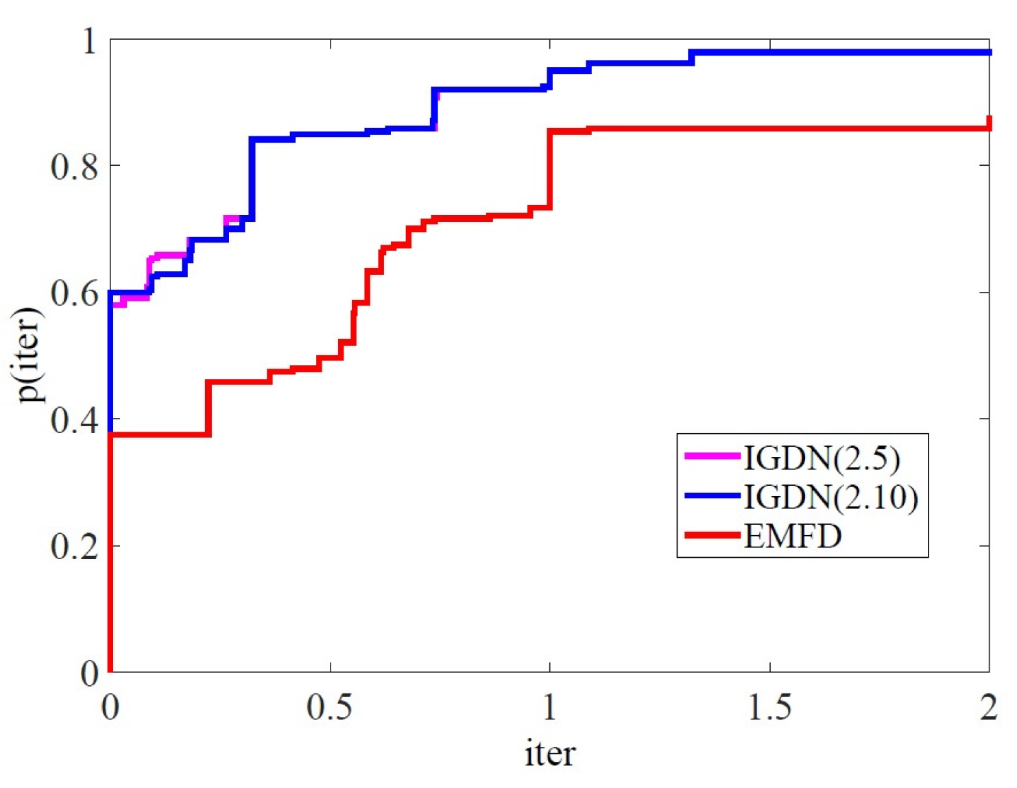
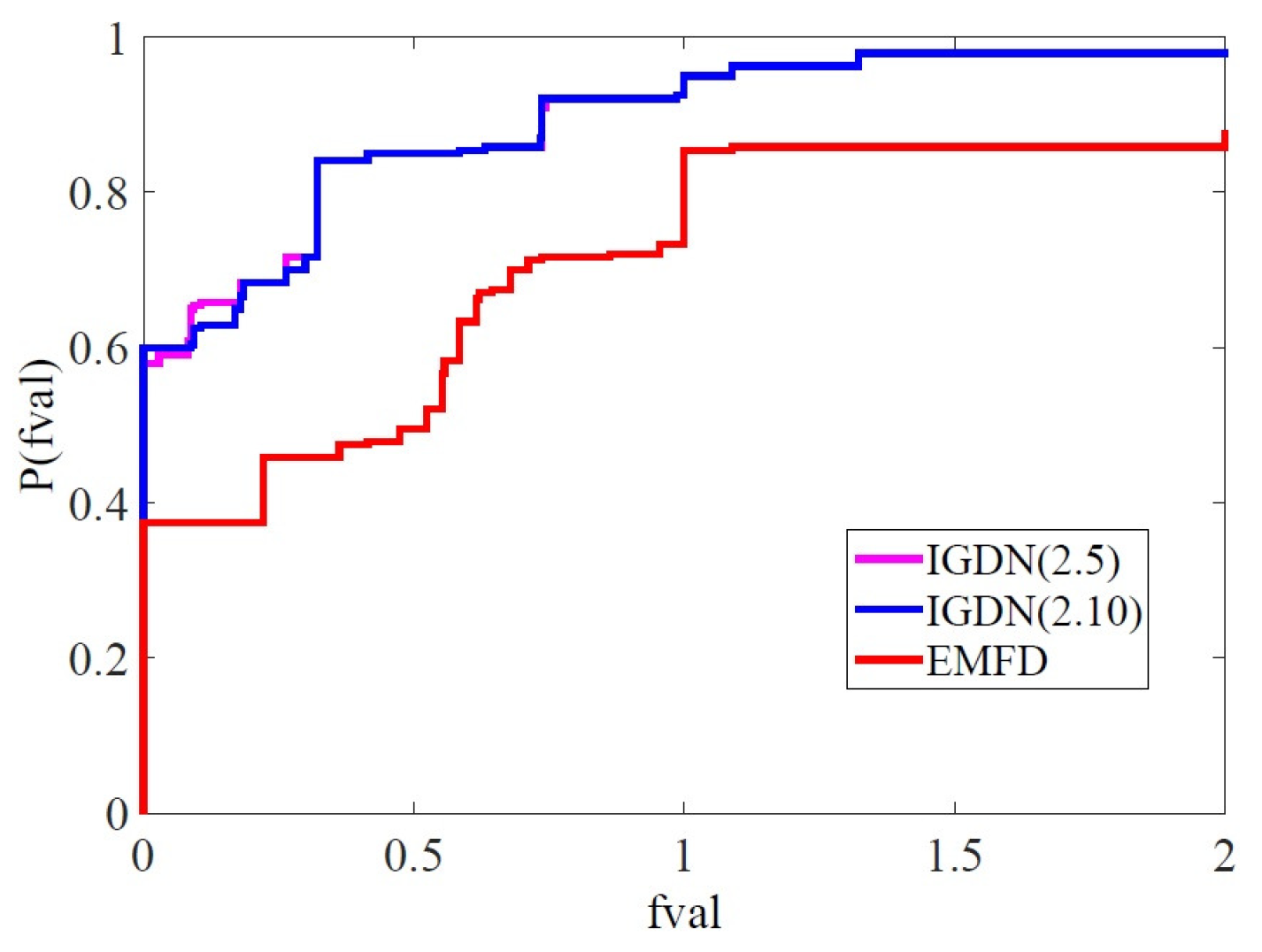
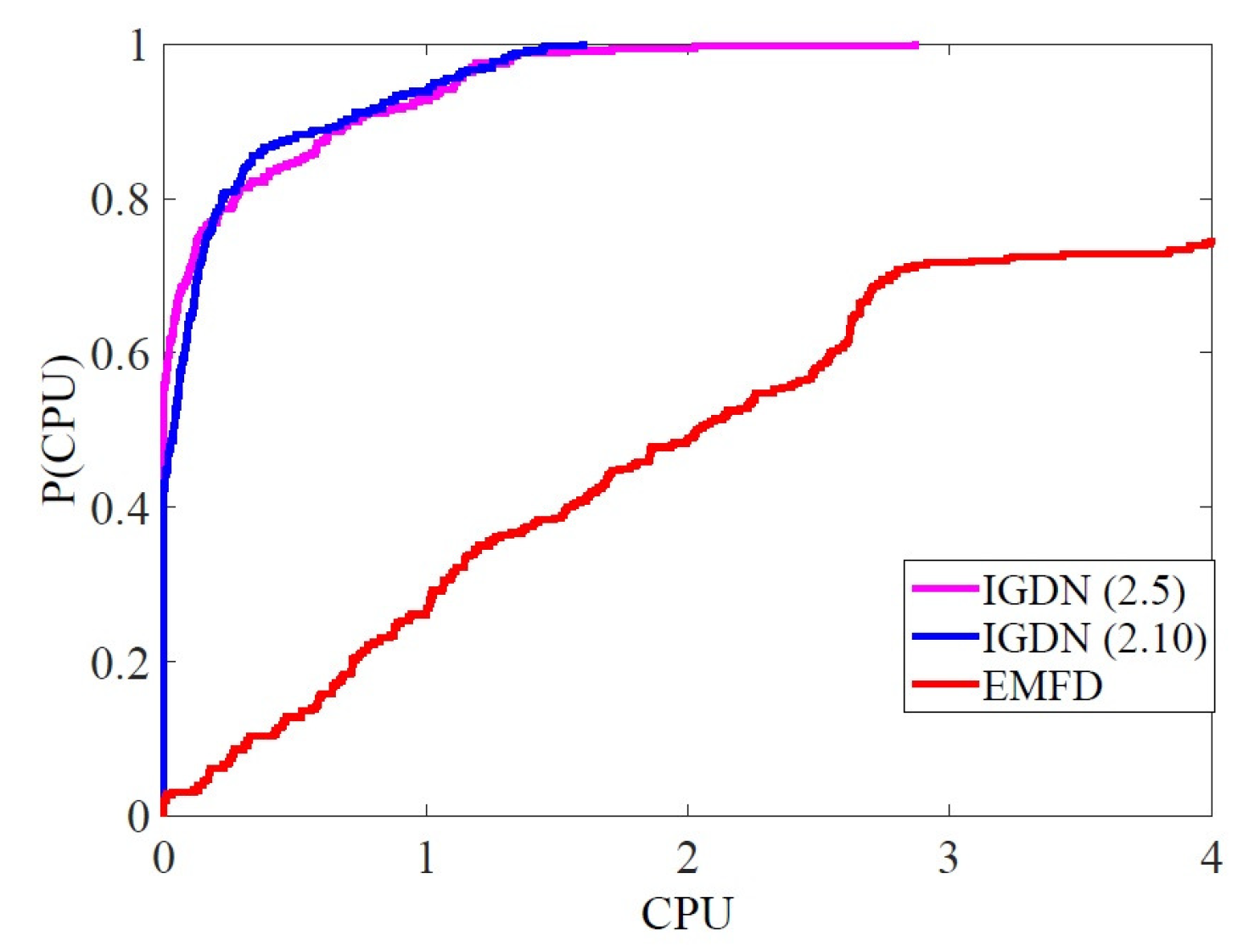
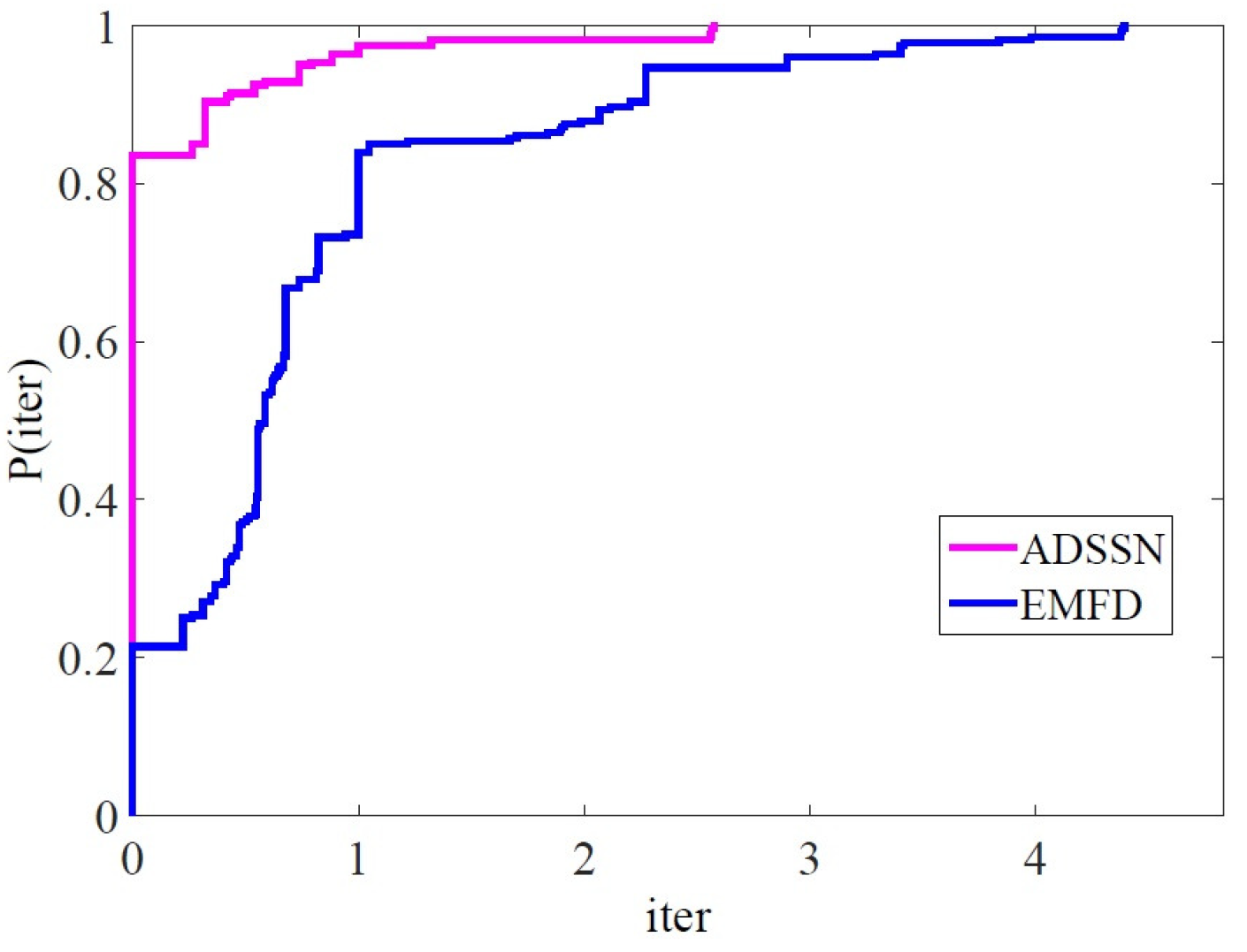
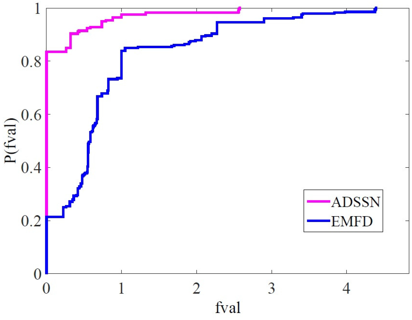
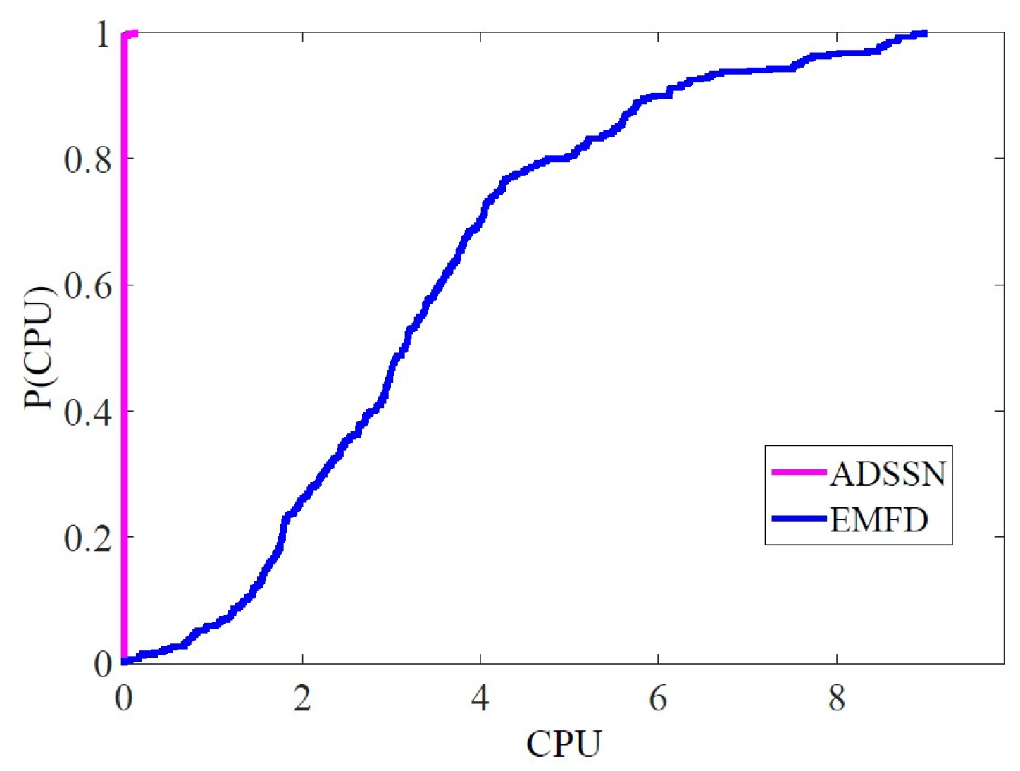
4. Numerical Experience

In order to confirm the efficiency of the presented $IGDN$ and $ADSSN$ processes, we compare them with the $EMFD$ iterations from [8]. We explore performances of both $IGDN$ variants defined by Algorithm 1, depending on chosen acceleration parameter ${\gamma }_k$. These variants are denoted as $IGDN$ (29) and $IGDN$ (34).

The following values of needed parameters are used:

• $IGDN$ algorithms are defined using ${\omega }_1={\omega }_2={10}^{-4}$, ${\alpha }_0=0.01$, $s=0.2$, $ϵ={10}^{-4}$, and ${\eta }_k=\frac{1}{{(k+1)}^2}.$
• $EMFD$ method is defined using ${\omega }_1={\omega }_2={10}^{-4}$, ${\alpha }_0=0.01$, $s=0.2$, $ϵ={10}^{-4}$, and ${\eta }_k=\frac{1}{{(k+1)}^2}$.

We use the following initial points (IP shortly) for the iterations:

${\mathbf{x}}_1=ones(1,\dots ,1)$, ${\mathbf{x}}_2=\left(1,\frac{1}{2},\frac{1}{3},\dots ,\frac{1}{n}\right)$, ${\mathbf{x}}_3=(0.1,0.1,\dots ,0.1)$, ${\mathbf{x}}_4=(\frac{1}{n},\frac{2}{n},\dots ,1)$,

${\mathbf{x}}_5=\left(1-\frac{1}{n},1-\frac{2}{n},\dots ,0\right)$, ${\mathbf{x}}_6=(-1,\dots ,-1)$, ${\mathbf{x}}_7=\left(n-\frac{1}{n},n-\frac{2}{n},\dots ,n-1\right)$, ${\mathbf{x}}_8=(\frac{1}{2},1,\frac{2}{3},\dots ,\frac{2}{n})$.

The considered nine test problems are listed below.

Problem 1 (P1) [86] Nonsmooth Function

$F\left({\mathbf{x}}_i\right)=2{\mathbf{x}}_i-sin\left|{\mathbf{x}}_i\right|$, for $i=1,2,\dots ,n$.

Problem 2 (P2) [87]

$F\left({\mathbf{x}}_i\right)=min\left\{min({\mathbf{x}}_i,{\mathbf{x}}_i^2),max(\left|{\mathbf{x}}_i\right|,{\mathbf{x}}_i^3)\right\}$, $i=2,3,\cdots ,n$.

Problem 3 (P3) [87] Strictly Convex Function I

$F\left({\mathbf{x}}_i\right)=exp\left({\mathbf{x}}_i\right)-1$, for $i=1,2,\dots ,n$.

Problem 4 (P4) [87]

$F_1\left(\mathbf{x}\right)=h{\mathbf{x}}_1+{\mathbf{x}}_2-1,$

$F_i\left(\mathbf{x}\right)={\mathbf{x}}_{i-1}+h{\mathbf{x}}_i+{\mathbf{x}}_{i-1}-1,$$i=2,3,\dots ,n-1$, $h=2.5$

$F_n\left(\mathbf{x}\right)={\mathbf{x}}_{n-1}+h{\mathbf{x}}_n-1$.

Problem 5 (P5) [87]

$F_1\left(\mathbf{x}\right)={\mathbf{x}}_1+exp(cos(h{\mathbf{x}}_1+{\mathbf{x}}_2)),$

$F_i\left(\mathbf{x}\right)={\mathbf{x}}_i+exp(cos(h{\mathbf{x}}_{i-1}+{\mathbf{x}}_i+{\mathbf{x}}_{i+1})),$ for $i=2,3,\dots ,n-1$, $h=\frac{1}{n+1}$

$F_n\left(\mathbf{x}\right)={\mathbf{x}}_n+exp(cos(h{\mathbf{x}}_{n-1}+{\mathbf{x}}_n))$

Problem 6 (P6) [87]

$F_1\left(\mathbf{x}\right)=2{\mathbf{x}}_1+sin\left(\mathbf{x}\right)-1,$

$F_i\left(\mathbf{x}\right)=-2{\mathbf{x}}_{i-1}+2{\mathbf{x}}_i+2sin\left({\mathbf{x}}_i\right)-1,$ for $i=2,3,\dots ,n-1$, $h=2.5$

$F_n\left(\mathbf{x}\right)=-2{\mathbf{x}}_n+sin\left({\mathbf{x}}_n\right)-1$.

Problem 7 (P7) [87]

$F_1\left(\mathbf{x}\right)=3{\mathbf{x}}_1^3+{\mathbf{x}}_2-5+sin({\mathbf{x}}_1-{\mathbf{x}}_2)sin({\mathbf{x}}_1+{\mathbf{x}}_2),$

$F_i\left(\mathbf{x}\right)=3{\mathbf{x}}_i^3+2{\mathbf{x}}_{i+1}-5sin({\mathbf{x}}_i-{\mathbf{x}}_{i+1})+4{\mathbf{x}}_i-{\mathbf{x}}_{i-1}exp({\mathbf{x}}_{i-1}-{\mathbf{x}}_i)-3,$ for $i=2,3,\dots ,n-1$,

$F_n\left(\mathbf{x}\right)=-{\mathbf{x}}_{n-1}exp({\mathbf{x}}_{n-1}-{\mathbf{x}}_n)+4{\mathbf{x}}_n-3$.

Problem 8 (P8) [86]

$F\left({\mathbf{x}}_i\right)={\mathbf{x}}_i-sin\left|{\mathbf{x}}_i-1\right|$, for $i=1,2,\dots ,n$.

Problem 9 (P9) [86]

$F\left({\mathbf{x}}_i\right)=2{\mathbf{x}}_i-sin\left|{\mathbf{x}}_i\right|$, for $i=1,2,\dots ,n$.

All tested methods are analyzed concerning three main computational aspects: number of iterations (iter), number of function evaluations (fval), and the CPU time (CPU). Performances of analyzed models are investigated on nine listed problems, applied on eight marked initial points, for five variables: 1000, 5000, 10,000, 50,000, 100,000.

According to obtained results, $IGDN$ (29) and $IGDN$ (34) have better performances in comparison to the $EMFD$ method from [8]. Both variants of $IGDN$ algorithms outperform the $EMFD$ method in all considered performances. In the next

Table 1. IGDN-EMFD comparisons.

Methods	(29)	(34)	(29) = (34)	(29) = (34) = $\mathit{EMFD}$	$\mathit{EMFD}$	$\mathit{IGDN}$ Total
iter	52	32	181	23	72	265
fval	52	33	180	24	71	265
CPU (sec)	214	141	0	0	5	355

(IGDN-EMFD comparisons), we display the best comparative analysis achievements of all methods regarding three tested profiles: iter, fval, and CPU.

The $IGDN$ (29) variant gives the best results in 52 out of 360 cases, considering the minimal number of iterations. Further, $IGDN$ (34) has the lowest outcomes in 33 out of 230 cases. These variants have the same minimal number of iterations in total, 181 out of 360 cases. All tree models require equal minimal number of iterations in 23 out of 360 cases, while the $EMFD$ methods give the minimal number of iterations in 71 out of 360 cases. Considering the needed number of iterations, $IGDN$ variants reach the minimal values in 265 out of 360 cases, as stated in the column $IGDN$ total.

Regarding the fval metric, the results are as follows: 52 out of 360 cases are in favor to $IGDN$ (29), 33 out of 360 with respect to $IGDN$ (34), 180 out of 360 when both $IGDN$ variants have the same minimal fval, while in 24 out of 360 cases all three methods give equal fval minimal values, and 71 out of 360 are in favor to the $EMFD$ method. The total minimal fval values achieved under the application of some $IGDN$ variants are the same as the total minimal iter numbers, i.e., 265 out of 360.

Concerning the CPU time, numerical outcomes are absolutely in favor of $IGDN$ variants, i.e., in 355 out of 360 cases, while the $EMFD$ is faster only in 5 out of 360 outcomes.

Obtained numerical results justify better performance characteristics of the $ADSSN$ method, which is defined by Algorithm 3, compared to the $EMFD$ method. Actually, the $ADSSN$ scheme outperforms the $EMFD$ iteration regarding all analyzed metrics: iter, fval, CPU time, and additionally with respect to the norm of the objective function. The summary review of obtained numerical values is presented in

Table 2. IADSSN-EMFD comparisons.

Methods	ADSSN	EMFD	ADSSN = EMFD
iter	282	55	23
fval	281	56	23
CPU (sec)	359	1	0

(ADSSN-EMFD comparisons).

Results arranged in Table 2 confirm huge dominance of the $ADSSN$ scheme in comparison with the $EMFD$ method. Considering the number of iterations, the $ADSSN$ method obtains 282 minimal values, while the $EMFD$ wins in only 55 instances. Similar outcomes are recorded regarding the fval profile. The most convincing results are achieved considering the CPU time metric, by which the $ADSSN$ model outperforms the $EMFD$ in 359 out of 360 cases.

This section finishes with a graphical analysis of the performance features of the considered methods. In the subsequent Figure 1, Figure 2, Figure 3, Figure 4, Figure 5 and Figure 6, we display Dolan and Moré [88] performance profiles of compared models in relation to tested metrics: iter, fval, and CPU.

Figure 1, Figure 2 and Figure 3 exhibit the clear superiority of $IGDN$ (29) and $IGDN$ (34) iterations compared to corresponding $EMFD$ iterations regarding the analyzed characteristics iter (resp. fval, CPU time). Further, the theoretical equivalence between $IGDN$ (29) and $IGDN$ (34) implies their identical responses on testing criteria iter and fval, represented in Figure 1 and Figure 2. However, Figure 3 demonstrates slightly better performances of $IGDN$ (34) with respect to $IGDN$ (29), which implies that the updating rule (34) is slightly better compared to (29) concerning the execution time. So, $IGDN$ (34) is computationally the most effective algorithm.

In the rest of this section, we compare $ADSSN$ and $EMFD$.

Figure 4, Figure 5 and Figure 6 exhibit clear superiority of $ADSSN$ iterations compared to corresponding $EMFD$ iterations regarding all three analyzed performance profiles, iter, fval, and CPU.

5. Conclusions

The traditional gradient descent optimization schemes for solving SNE form a class of methods termed the $GDN$ class. A single step size parameter characterizes methods belonging to that class. We aim to upgrade the traditional $GDN$ iterates by introducing the improved gradient descent iterations ($IGDN$), which include complex steplength values defined by several parameters. In this way, we justified the assumption that applying two or more quantities in defining the composed step size parameters generally improves the performance of an underlying iterative process.

Numerical results confirm the evident superiority of $IGDN$ methods in comparison with $EMFD$ iterations from [8], which indicates the superiority of $IGDN$ methods over traditional $GDN$ methods considering all three analyzed features: iter, fval, and CPU. Confirmation of excellent performance of the presented models is also given through graphically displayed Dolan and Moré’s performance profiles.

The problem of solving SNE by applying some efficient accelerated gradient optimization models is of great interest to the optimization community. In that regard, the question of further upgrading $IGDN$, $ADDN$, and $ADSSN$ type of methods is still open.

One possibility for further research is proper exploitation of the results presented in Theorems 1–2 in defining proper updates of the scaling parameter ${\gamma }_k$. In addition, it will be interesting to examine and exploit similar results in solving classical nonlinear optimization problems.

References

1. Yuan, G.; Lu, X. A new backtracking inexact BFGS method for symmetric nonlinear equations. Comput. Math. Appl. 2008, 55, 116–129. [Google Scholar] [CrossRef] [Green Version]
2. Abubakar, A.B.; Kumam, P. An improved three–term derivative–free method for solving nonlinear equations. Comput. Appl. Math. 2018, 37, 6760–6773. [Google Scholar] [CrossRef]
3. Cheng, W. A PRP type method for systems of monotone equations. Math. Comput. Model. 2009, 50, 15–20. [Google Scholar] [CrossRef]
4. Hu, Y.; Wei, Z. Wei–Yao–Liu conjugate gradient projection algorithm for nonlinear monotone equations with convex constraints. Int. J. Comput. Math. 2015, 92, 2261–2272. [Google Scholar] [CrossRef]
5. La Cruz, W. A projected derivative–free algorithm for nonlinear equations with convex constraints. Optim. Methods Softw. 2014, 29, 24–41. [Google Scholar] [CrossRef]
6. La Cruz, W. A spectral algorithm for large–scale systems of nonlinear monotone equations. Numer. Algorithms 2017, 76, 1109–1130. [Google Scholar] [CrossRef]
7. Papp, Z.; Rapajić, S. FR type methods for systems of large–scale nonlinear monotone equations. Appl. Math. Comput. 2015, 269, 816–823. [Google Scholar] [CrossRef]
8. Halilu, A.S.; Waziri, M.Y. En enhanced matrix-free method via double steplength approach for solving systems of nonlinear equations. Int. J. Appl. Math. Res. 2017, 6, 147–156. [Google Scholar] [CrossRef] [Green Version]
9. Halilu, A.S.; Waziri, M.Y. A transformed double steplength method for solving large-scale systems of nonlinear equations. J. Numer. Math. Stochastics 2017, 9, 20–32. [Google Scholar]
10. Waziri, M.Y.; Muhammad, H.U.; Halilu, A.S.; Ahmed, K. Modified matrix-free methods for solving system of nonlinear equations. Optimization 2021, 70, 2321–2340. [Google Scholar] [CrossRef]
11. Osinuga, I.A.; Dauda, M.K. Quadrature based Broyden-like method for systems of nonlinear equations. Stat. Optim. Inf. Comput. 2018, 6, 130–138. [Google Scholar] [CrossRef]
12. Muhammad, K.; Mamat, M.; Waziri, M.Y. A Broyden’s-like method for solving systems of nonlinear equations. World Appl. Sci. J. 2013, 21, 168–173. [Google Scholar]
13. Ullah, N.; Sabi’u, J.; Shah, A. A derivative–free scaling memoryless Broyden–Fletcher–Goldfarb–Shanno method for solving a system of monotone nonlinear equations. Numer. Linear Algebra Appl. 2021, 28, e2374. [Google Scholar] [CrossRef]
14. Abubakar, A.B.; Kumam, P. A descent Dai–Liao conjugate gradient method for nonlinear equations. Numer. Algorithms 2019, 81, 197–210. [Google Scholar] [CrossRef]
15. Aji, S.; Kumam, P.; Awwal, A.M.; Yahaya, M.M.; Kumam, W. Two Hybrid Spectral Methods With Inertial Effect for Solving System of Nonlinear Monotone Equations With Application in Robotics. IEEE Access 2021, 9, 30918–30928. [Google Scholar] [CrossRef]
16. Dauda, M.K.; Usman, S.; Ubale, H.; Mamat, M. An alternative modified conjugate gradient coefficient for solving nonlinear system of equations. Open J. Sci. Technol. 2019, 2, 5–8. [Google Scholar] [CrossRef]
17. Zheng, L.; Yang, L.; Liang, Y. A conjugate gradient projection method for solving equations with convex constraints. J. Comput. Appl. Math. 2020, 375, 112781. [Google Scholar] [CrossRef]
18. Waziri, M.Y.; Aisha, H.A. A diagonal quasi-Newton method for system of nonlinear equations. Appl. Math. Comput. Sci. 2014, 6, 21–30. [Google Scholar]
19. Waziri, M.Y.; Leong, W.J.; Hassan, M.A.; Monsi, M. Jacobian computation-free Newton’s method for systems of nonlinear equations. J. Numer. Math. Stochastics 2010, 2, 54–63. [Google Scholar]
20. Waziri, M.Y.; Majid, Z.A. An improved diagonal Jacobian approximation via a new quasi-Cauchy condition for solving large-scale systems of nonlinear equations. J. Appl. Math. 2013, 2013, 875935. [Google Scholar] [CrossRef] [Green Version]
21. Abdullah, H.; Waziri, M.Y.; Yusuf, S.O. A double direction conjugate gradient method for solving large-scale system of nonlinear equations. J. Math. Comput. Sci. 2017, 7, 606–624. [Google Scholar]
22. Yan, Q.-R.; Peng, X.-Z.; Li, D.-H. A globally convergent derivative-free method for solving large-scale nonlinear monotone equations. J. Comput. Appl. Math. 2010, 234, 649–657. [Google Scholar] [CrossRef] [Green Version]
23. Leong, W.J.; Hassan, M.A.; Yusuf, M.W. A matrix-free quasi-Newton method for solving large-scale nonlinear systems. Comput. Math. Appl. 2011, 62, 2354–2363. [Google Scholar] [CrossRef] [Green Version]
24. Waziri, M.Y.; Leong, W.J.; Mamat, M. A two-step matrix-free secant method for solving large-scale systems of nonlinear equations. J. Appl. Math. 2012, 2012, 348654. [Google Scholar] [CrossRef] [Green Version]
25. Waziri, M.Y.; Leong, W.J.; Hassan, M.A.; Monsi, M. A new Newton’s Method with diagonal Jacobian approximation for systems of nonlinear equations. J. Math. Stat. 2010, 6, 246–252. [Google Scholar] [CrossRef]
26. Waziri, M.Y.; Leong, W.J.; Mamat, M.; Moyi, A.U. Two-step derivative-free diagonally Newton’s method for large-scale nonlinear equations. World Appl. Sci. J. 2013, 21, 86–94. [Google Scholar]
27. Yakubu, U.A.; Mamat, M.; Mohamad, M.A.; Rivaie, M.; Sabi’u, J. A recent modification on Dai–Liao conjugate gradient method for solving symmetric nonlinear equations. Far East J. Math. Sci. 2018, 103, 1961–1974. [Google Scholar] [CrossRef]
28. Uba, L.Y.; Waziri, M.Y. Three-step derivative-free diagonal updating method for solving large-scale systems of nonlinear equations. J. Numer. Math. Stochastics 2014, 6, 73–83. [Google Scholar]
29. Zhou, Y.; Wu, Y.; Li, X. A New Hybrid PRPFR Conjugate Gradient Method for Solving Nonlinear Monotone Equations and Image Restoration Problems. Math. Probl. Eng. 2020, 2020, 6391321. [Google Scholar] [CrossRef]
30. Waziri, M.Y.; Leong, W.J.; Mamat, M. An efficient solver for systems of nonlinear equations with singular Jacobian via diagonal updating. Appl. Math. Sci. 2010, 4, 3403–3412. [Google Scholar]
31. Waziri, M.Y.; Leong, W.J.; Hassan, M.A. Diagonal Broyden-like method for large-scale systems of nonlinear equations. Malays. J. Math. Sci. 2012, 6, 59–73. [Google Scholar]
32. Abubakar, A.B.; Sabi’u, J.; Kumam, P.; Shah, A. Solving nonlinear monotone operator equations via modified SR1 update. J. Appl. Math. Comput. 2021, 67, 343–373. [Google Scholar] [CrossRef]
33. Grosan, C.; Abraham, A. A new approach for solving nonlinear equations systems. IEEE Trans. Syst. Man Cybern. 2008, 38, 698–714. [Google Scholar] [CrossRef]
34. Dehghan, M.; Hajarian, M. New iterative method for solving nonlinear equations with fourth-order convergence. Int. J. Comput. Math. 2010, 87, 834–839. [Google Scholar] [CrossRef]
35. Dehghan, M.; Hajarian, M. Fourth-order variants of Newton’s method without second derivatives for solving nonlinear equations. Eng. Comput. 2012, 29, 356–365. [Google Scholar] [CrossRef]
36. Kaltenbacher, B.; Neubauer, A.; Scherzer, O. Iterative Regularization Methods for Nonlinear III—Posed Problems; De Gruyter: Berlin, Germany; New York, NY, USA, 2008. [Google Scholar]
37. Wang, Y.; Yuan, Y. Convergence and regularity of trust region methods for nonlinear ill-posed problems. Inverse Probl. 2005, 21, 821–838. [Google Scholar] [CrossRef] [Green Version]
38. Dehghan, M.; Hajarian, M. Some derivative free quadratic and cubic convergence iterative formulas for solving nonlinear equations. Comput. Appl. Math. 2010, 29, 19–30. [Google Scholar] [CrossRef]
39. Dehghan, M.; Hajarian, M. On some cubic convergence iterative formulae without derivatives for solving nonlinear equations. Int. J. Numer. Methods Biomed. Eng. 2011, 27, 722–731. [Google Scholar] [CrossRef]
40. Dehghan, M.; Shirilord, A. Accelerated double-step scale splitting iteration method for solving a class of complex symmetric linear systems. Numer. Algorithms 2020, 83, 281–304. [Google Scholar] [CrossRef]
41. Dehghan, M.; Shirilord, A. A generalized modified Hermitian and skew-Hermitian splitting (GMHSS) method for solving complex Sylvester matrix equation. Appl. Math. Comput. 2019, 348, 632–651. [Google Scholar] [CrossRef]
42. Bellavia, S.; Gurioli, G.; Morini, B.; Toint, P.L. Trust-region algorithms: Probabilistic complexity and intrinsic noise with applications to subsampling techniques. EURO J. Comput. Optim. 2022, 10, 100043. [Google Scholar] [CrossRef]
43. Bellavia, S.; Krejić, N.; Morini, B.; Rebegoldi, S. A stochastic first-order trust-region method with inexact restoration for finite-sum minimization. Comput. Optim. Appl. 2023, 84, 53–84. [Google Scholar] [CrossRef]
44. Bellavia, S.; Krejić, N.; Morini, B. Inexact restoration with subsampled trust-region methods for finite-sum minimization. Comput. Optim. Appl. 2020, 76, 701–736. [Google Scholar] [CrossRef]
45. Eshaghnezhad, M.; Effati, S.; Mansoori, A. A Neurodynamic Model to Solve Nonlinear Pseudo-Monotone Projection Equation and Its Applications. IEEE Trans. Cybern. 2017, 47, 3050–3062. [Google Scholar] [CrossRef]
46. Meintjes, K.; Morgan, A.P. A methodology for solving chemical equilibrium systems. Appl. Math. Comput. 1987, 22, 333–361. [Google Scholar] [CrossRef]
47. Crisci, S.; Piana, M.; Ruggiero, V.; Scussolini, M. A regularized affine–acaling trust–region method for parametric imaging of dynamic PET data. SIAM J. Imaging Sci. 2021, 14, 418–439. [Google Scholar] [CrossRef]
48. Bonettini, S.; Zanella, R.; Zanni, L. A scaled gradient projection method for constrained image deblurring. Inverse Probl. 2009, 25, 015002. [Google Scholar] [CrossRef] [Green Version]
49. Liu, J.K.; Du, X.L. A gradient projection method for the sparse signal reconstruction in compressive sensing. Appl. Anal. 2018, 97, 2122–2131. [Google Scholar] [CrossRef]
50. Liu, J.K.; Li, S.J. A projection method for convex constrained monotone nonlinear equations with applications. Comput. Math. Appl. 2015, 70, 2442–2453. [Google Scholar] [CrossRef]
51. Xiao, Y.; Zhu, H. A conjugate gradient method to solve convex constrained monotone equations with applications in compressive sensing. J. Math. Anal. Appl. 2013, 405, 310–319. [Google Scholar] [CrossRef]
52. Awwal, A.M.; Wang, L.; Kumam, P.; Mohammad, H.; Watthayu, W. A Projection Hestenes–Stiefel Method with Spectral Parameter for Nonlinear Monotone Equations and Signal Processing. Math. Comput. Appl. 2020, 25, 27. [Google Scholar] [CrossRef]
53. Fukushima, M. Equivalent differentiable optimization problems and descent methods for asymmetric variational inequality problems. Math. Program. 1992, 53, 99–110. [Google Scholar] [CrossRef]
54. Qian, G.; Han, D.; Xu, L.; Yang, H. Solving nonadditive traffic assignment problems: A self-adaptive projection–auxiliary problem method for variational inequalities. J. Ind. Manag. Optim. 2013, 9, 255–274. [Google Scholar] [CrossRef]
55. Ghaddar, B.; Marecek, J.; Mevissen, M. Optimal power flow as a polynomial optimization problem. IEEE Trans. Power Syst. 2016, 31, 539–546. [Google Scholar] [CrossRef] [Green Version]
56. Ivanov, B.; Stanimirović, P.S.; Milovanović, G.V.; Djordjević, S.; Brajević, I. Accelerated multiple step-size methods for solving unconstrained optimization problems. Optim. Methods Softw. 2021, 36, 998–1029. [Google Scholar] [CrossRef]
57. Andrei, N. An acceleration of gradient descent algorithm with backtracking for unconstrained optimization. Numer. Algorithms 2006, 42, 63–73. [Google Scholar] [CrossRef]
58. Stanimirović, P.S.; Miladinović, M.B. Accelerated gradient descent methods with line search. Numer. Algorithms 2010, 54, 503–520. [Google Scholar] [CrossRef]
59. Sun, W.; Yuan, Y.-X. Optimization Theory and Methods: Nonlinear Programming; Springer: New York, NY, USA, 2006. [Google Scholar]
60. Petrović, M.J. An Accelerated Double Step Size model in unconstrained optimization. Appl. Math. Comput. 2015, 250, 309–319. [Google Scholar] [CrossRef]
61. Petrović, M.J.; Stanimirović, P.S. Accelerated Double Direction method for solving unconstrained optimization problems. Math. Probl. Eng. 2014, 2014, 965104. [Google Scholar] [CrossRef]
62. Stanimirović, P.S.; Milovanović, G.V.; Petrović, M.J.; Kontrec, N. A Transformation of accelerated double step size method for unconstrained optimization. Math. Probl. Eng. 2015, 2015, 283679. [Google Scholar] [CrossRef] [Green Version]
63. Nocedal, J.; Wright, S.J. Numerical Optimization; Springer: New York, NY, USA, 1999. [Google Scholar]
64. Barzilai, J.; Borwein, J.M. Two-point step size gradient method. IMA J. Numer. Anal. 1988, 8, 141–148. [Google Scholar] [CrossRef]
65. Dai, Y.H. Alternate step gradient method. Optimization 2003, 52, 395–415. [Google Scholar] [CrossRef]
66. Dai, Y.H.; Fletcher, R. On the asymptotic behaviour of some new gradient methods. Math. Program. 2005, 103, 541–559. [Google Scholar] [CrossRef]
67. Dai, Y.H.; Liao, L.Z. R-linear convergence of the Barzilai and Borwein gradient method. IMA J. Numer. Anal. 2002, 22, 1–10. [Google Scholar] [CrossRef]
68. Dai, Y.H.; Yuan, J.Y.; Yuan, Y. Modified two-point step-size gradient methods for unconstrained optimization. Comput. Optim. Appl. 2002, 22, 103–109. [Google Scholar] [CrossRef]
69. Dai, Y.H.; Yuan, Y. Alternate minimization gradient method. IMA J. Numer. Anal. 2003, 23, 377–393. [Google Scholar] [CrossRef]
70. Dai, Y.H.; Yuan, Y. Analysis of monotone gradient methods. J. Ind. Manag. Optim. 2005, 1, 181–192. [Google Scholar] [CrossRef]
71. Dai, Y.H.; Zhang, H. Adaptive two-point step size gradient algorithm. Numer. Algorithms 2001, 27, 377–385. [Google Scholar] [CrossRef]
72. Raydan, M. On the Barzilai and Borwein choice of steplength for the gradient method. IMA J. Numer. Anal. 1993, 13, 321–326. [Google Scholar] [CrossRef]
73. Raydan, M. The Barzilai and Borwein gradient method for the large scale unconstrained minimization problem. SIAM J. Optim. 1997, 7, 26–33. [Google Scholar] [CrossRef]
74. Vrahatis, M.N.; Androulakis, G.S.; Lambrinos, J.N.; Magoulas, G.D. A class of gradient unconstrained minimization algorithms with adaptive step-size. J. Comput. Appl. Math. 2000, 114, 367–386. [Google Scholar] [CrossRef] [Green Version]
75. Yuan, Y. A new step size for the steepest descent method. J. Comput. Math. 2006, 24, 149–156. [Google Scholar]
76. Frassoldati, G.; Zanni, L.; Zanghirati, G. New adaptive step size selections in gradient methods. J. Ind. Manag. Optim. 2008, 4, 299–312. [Google Scholar] [CrossRef]
77. Serafino, D.; Ruggiero, V.; Toraldo, G.; Zanni, L. On the steplength selection in gradient methods for unconstrained optimization. Appl. Math. Comput. 2018, 318, 176–195. [Google Scholar] [CrossRef] [Green Version]
78. Crisci, S.; Porta, F.; Ruggiero, V.; Zanni, L. Spectral properties of Barzilai–Borwein rules in solving singly linearly constrained optimization problems subject to lower and upper bounds. SIAM J. Optim. 2020, 30, 1300–1326. [Google Scholar] [CrossRef]
79. Crisci, S.; Porta, F.; Ruggiero, V.; Zanni, L. Hybrid limited memory gradient projection methods for box–constrained optimization problems. Comput. Optim. Appl. 2023, 84, 151–189. [Google Scholar] [CrossRef]
80. Miladinović, M.; Stanimirović, P.S.; Miljković, S. Scalar Correction method for solving large scale unconstrained minimization problems. J. Optim. Theory Appl. 2011, 151, 304–320. [Google Scholar] [CrossRef]
81. Raydan, M.; Svaiter, B.F. Relaxed steepest descent and Cauchy-Barzilai-Borwein method. Comput. Optim. Appl. 2002, 21, 155–167. [Google Scholar] [CrossRef]
82. Djordjević, S.S. Two modifications of the method of the multiplicative parameters in descent gradient methods. Appl. Math. Comput. 2012, 218, 8672–8683. [Google Scholar]
83. Zhang, Y.; Yi, C. Zhang Neural Networks and Neural-Dynamic Method; Nova Science Publishers, Inc.: New York, NY, USA, 2011. [Google Scholar]
84. Zhang, Y.; Ma, W.; Cai, B. From Zhang neural network to Newton iteration for matrix inversion. IEEE Trans. Circuits Syst. I Regul. Pap. 2009, 56, 1405–1415. [Google Scholar] [CrossRef]
85. Djuranovic-Miličić, N.I.; Gardašević-Filipović, M. A multi-step curve search algorithm in nonlinear optimization - nondifferentiable case. Facta Univ. Ser. Math. Inform. 2010, 25, 11–24. [Google Scholar]
86. Zhou, W.J.; Li, D.H. A globally convergent BFGS method for nonlinear monotone equations without any merit functions. Math. Comput. 2008, 77, 2231–2240. [Google Scholar] [CrossRef]
87. La Cruz, W.; Martínez, J.; Raydan, M. Spectral residual method without gradient information for solving large-scale nonlinear systems of equations. Math. Comput. 2006, 75, 1429–1448. [Google Scholar] [CrossRef] [Green Version]
88. Dolan, E.; Moré, J. Benchmarking optimization software with performance profiles. Math. Program. 2002, 91, 201–213. [Google Scholar] [CrossRef]
Figure 1. Performance profile of I G D N versus E M F D [8] with respect to iter.
Algorithms 16 00064 g001
Figure 2. Performance profile of I G D N versus E M F D [8] with respect to fval.
Algorithms 16 00064 g002
Figure 3. Performance profile of I G D N versus E M F D [8] with respect to CPU.
Algorithms 16 00064 g003
Figure 4. Performance profile of A D S S N versus E M F D [8] with respect to iter.
Algorithms 16 00064 g004
Figure 5. Performance profile of A D S S N versus E M F D [8] with respect to fval.
Algorithms 16 00064 g005
Figure 6. Performance profile of A D S S N versus E M F D [8] with respect to CPU.
Algorithms 16 00064 g006