Article

Quadratic Multilinear Discriminant Analysis for Tensorial Data Classification

1
Department of Computational Medicine and Bioinformatics, University of Michigan, Ann Arbor, MI 48109, USA
2
Computer Science Department, Queen’s College, CUNY, New York, NY 11367, USA
3
Michigan Institute for Data Science (MIDAS), University of Michigan, Ann Arbor, MI 48109, USA
4
Michigan Center for Integrative Research in Critical Care (MCIRCC), University of Michigan, Ann Arbor, MI 48109, USA
5
Emergency Medicine, University of Michigan, Ann Arbor, MI 48109, USA
6
Mathematics Department, Northeastern University, Boston, MA 02115, USA
*
Author to whom correspondence should be addressed.
Algorithms 2023, 16(2), 104; https://doi.org/10.3390/a16020104
Submission received: 10 January 2023 / Revised: 7 February 2023 / Accepted: 10 February 2023 / Published: 11 February 2023
(This article belongs to the Section Algorithms for Multidisciplinary Applications)

Abstract

:
Over the past decades, there has been an increase of attention to adapting machine learning methods to fully exploit the higher order structure of tensorial data. One problem of great interest is tensor classification, and in particular the extension of linear discriminant analysis to the multilinear setting. We propose a novel method for multilinear discriminant analysis that is radically different from the ones considered so far, and it is the first extension to tensors of quadratic discriminant analysis. Our proposed approach uses invariant theory to extend the nearest Mahalanobis distance classifier to the higher-order setting, and to formulate a well-behaved optimization problem. We extensively test our method on a variety of synthetic data, outperforming previously proposed MDA techniques. We also show how to leverage multi-lead ECG data by constructing tensors via taut string, and use our method to classify healthy signals versus unhealthy ones; our method outperforms state-of-the-art MDA methods, especially after adding significant levels of noise to the signals. Our approach reached an AUC of 0.95 ( 0.03 ) on clean signals—where the second best method reached 0.91 ( 0.03 ) —and an AUC of 0.89 ( 0.03 ) after adding noise to the signals (with a signal-to-noise-ratio of 30 )—where the second best method reached 0.85 ( 0.05 ) . Our approach is fundamentally different than previous work in this direction, and proves to be faster, more stable, and more accurate on the tests we performed.

1. Introduction

Data often has a higher-order structure, and leveraging this structure can significantly improve the results of the problem at hand. However, many machine learning methods do not naturally extend to tensors in a way that account for this tensorial structure. In the case of classification problems, for example, there has been tremendous interest in extending linear discriminant analysis (LDA) to the tensorial setting. LDA is a classical and versatile method for classification, but is typically not well suited for data in matrix or in tensor forms (higher-order matrices). These types of data, with a higher order structure, are very common nowadays and there has been a lot of interest in developing machine learning methods that can leverage this structure. Natural examples of data in matrix form are black-and-white images and multi-lead electrocardiogram (ECG) readings. Similarly, color images, videos, and data in matrix forms that vary with time are examples of third order tensors. Classifying matrix data with LDA (or other vector-based classical machine learning algorithms) requires the data to be vectorized first; this often leads to large vectors, but—perhaps more importantly—also causes the loss of important information such as spatial locality. Furthermore, vectorization ignores the multilinear structure of the data. For example, a matrix of rank one depends on fewer parameters than a full-rank matrix. On top of that, matrices from different classes might have different ranks, so using the multilinear structure might help in the classification task. These considerations apply even more strongly to higher-order data, and tensor techniques have been successfully applied in a variety of classification settings such as images (see [1]), electroencephalogram (EEG) data (see [2,3]), and ECG signals (see [4,5]); for a recent survey of applications to clinical informatics, see [6]. On the other hand, tensors of order 3 or more enjoy many good properties (e.g., unique decompositions), so that sometimes it is in fact advantageous to reshape data given in form of vectors or matrices into data of higher order [7].
For these reasons, there has been intensive work in recent years on extending LDA to multilinear discriminant analysis (MDA) to leverage the multilinear structure of the data. Using the Fisher criterion for LDA, given data points x 1 , , x m R n belonging to two classes C 1 , C 2 of size m 1 , m 2 , one seeks the optimal projection to a hyperplane that maximizes distances between different classes (measured by the between-class scatter matrix) and minimizes distances within the same class (measured by the within-class scatter matrix). If  μ 1 , μ 2 are the means for each class and μ is the overall mean, one can define the scatter matrix for class i as the covariance matrix for that class,
S i = 1 m i j C i ( x j μ i ) ( x j μ i ) t ,
the within class scatter matrix as S W = S 1 + S 2 , and the between class scatter matrix as
S B = m 1 ( μ 1 μ ) ( μ 1 μ ) t + m 2 ( μ 2 μ ) ( μ 2 μ ) t .
The hyperplane f ( x ) = w t x to project onto is then obtained by maximizing
J ( w ) = w t S B w w t S W w .
In an attempt to extend Fisher’s approach, most MDA methods seek to project tensor data to a lower dimensional vector or tensor space by similarly maximizing distances between classes while simultaneously minimizing distances within the same class. Early work [8,9,10] considered the case of matrix data. After that, many methods have been proposed for tensorial data, usually introducing between-class and within-class scatter matrices for each mode. Different methods consider various functions to optimize (like the scatter-ratio criterion or the scatter-difference criterion from Fisher discriminant analysis), and propose different algorithms to optimize them. Discriminant analysis with tensor representation (DATER) [11], generalized eigenvalue discriminant analysis with tensor representation (DATEReig) [12] and constrained multilinear discriminant analysis (CMDA) [1] seek to maximize the scatter-ratio criterion iteratively by alternating through each mode; direct general tensor discriminant analysis (DGTDA) [1] seeks to maximize the scatter difference directly. The methods proposed in [3], such as manifold Tucker discriminant analysis (ManTDA) and manifold PARAFAC discriminant analysis (ManPDA), seek to optimize simultaneously, in all modes, the projection matrices over a product of Stiefel manifolds with respect to the scatter-ratio criterion or its simplified trace ratio objective.
However, the optimization problems considered so far are ill-behaved in general due to the existence of local optima. Because of this, several iterations with different random initializations are sometimes necessary to try to avoid such local optima. However, this adds to the computational cost of the method, while still having no guarantee the computed solution is a global optimum. Furthermore, the performance of these methods drastically depends on the choice of the dimensions of the space to project onto. For example, a tensor of size 10 × 10 × 10 can be projected onto a tensor of size p × q × r with 1 p , q , r 10 . This amounts to, in principle, 1000 possibilities. In practice, one usually chooses all dimensions to be equal, but if the size of tensor varies greatly from one mode to the other, this option is not viable. Therefore these methods include the additional cost of determining the best dimensions to project onto. We will see that our proposed method does not share these issues, since instead of projecting onto a lower dimensional subspace we look for a change of coordinates in the given space.
In this paper, we take a radically different approach: Kempf–Ness multilinear discriminant analysis (KNMDA). Starting from the interpretation of classic LDA as a nearest Mahalanobis distance classifier, we reformulate LDA by means of invariant theory, which allows us to extend it naturally to structured data in the form of a well-behaved optimization problem. In fact, our framework allows us to also reformulate quadratic discriminant analysis (QDA) by means of invariant theory, and to extend QDA to tensorial data for the first time.
Invariant theory, originating in 19th century and modernized by David Hilbert, can be applied to many areas of computer science, such as coding theory [13] and computer vision [14,15]. Some newer applications more relevant to this study are those related to scaling algorithms [16], matrix and tensor completion [17], and maximum likelihood estimation [18]. In invariant theory, one studies the linear action of groups on vector spaces and polynomials that are invariant under these group symmetries.
A major tool of invariant theory is the Kempf–Ness theorem [19]. Roughly speaking, the theorem states that if an orbit has a point that is closest to the origin, then this point is essentially unique. This translates to a certain optimization problem having a unique optimal solution. This result of Kempf–Ness theory provides a natural extension of LDA to the higher order setting.
LDA is related to the Mahalanobis distance: it can be interpreted as a k-means algorithm, where we classify a data point based on the smallest distance from the mean of the training data of each class, and the distance is given by the Mahalanobis one. In turn, the Mahalanobis distance of a point x from the mean of the training data x ¯ can be thought of as Euclidean distance after a suitable change of coordinates, namely Σ 1 / 2 ( x x ¯ ) , where Σ is the sample covariance matrix across the entire training dataset. Therefore, we can interpret LDA as a k-means algorithm in a suitable coordinate system. By allowing different sample covariance matrices for each class—i.e., different sets of coordinates for each class—we can similarly interpret QDA in this framework. If  X is a matrix (or tensor), applying a change of coordinates after vectorization might radically alter the structure of X . This can be especially nefarious when the data is sparse, e.g., it has low rank or few non-zero entries. To solve this issue, we can apply a different change of coordinates in each mode of X , i.e., multiply by an invertible matrix in each mode. This strategy would preserve the rank. To further preserve the structure of the data, one might want to consider coordinate changes that preserve volumes; therefore we will consider invertible matrices with the determinant 1. The restriction to matrices with determinant 1 does not have a large impact on the method, as it amounts to rescaling an invertible matrix to make its determinant equal to 1. The question now is how to appropriately choose such a change of coordinates. The Kempf–Ness theory gives us a choice of coordinates by solving a well-behaved optimization problem which reduces to Mahalanobis distance in the case of vectorial data.
The proposed method was tested on synthetic data of several types, some of which have already appeared in the literature [3,20]. The results demonstrate that there are classes of data on which the proposed method achieves significantly better results than other existing methods. The method was also employed to classify tensors extracted from ECG signals. The analysis of ECG recordings with tensor-based approaches has proven to be very fruitful in a variety of settings, such as the detection and localization of myocardial infarction, irregular heartbeat classification, ECG data compression, detection and quantification of T-wave alternans, and analysis of changes in heartbeat morphology (see [
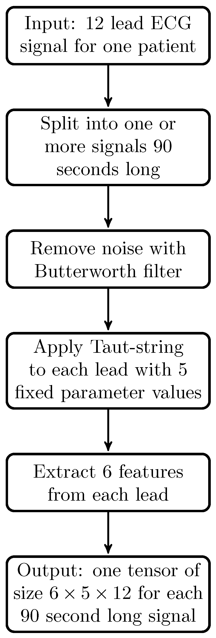
4] for an overview). In our experiments, we consider third-order tensors extracted from multi-lead ECG signals from the publicly available PhysioNet PTB dataset [21]. There are several ways of constructing tensors from ECG data; here we follow the approach of [22] by extracting features from taut-string approximations of the signals. In [22], feature vectors were extracted from ECG signals via taut string as well as other methods, and then classification was performed with standard machine learning techniques, among which linear support vector machine (SVM) performed best. We found that the same applies to our experiments, which is why in the comparisons we also include the results of an SVM classifier on the vectorized tensors. We believe that the method by which we construct third-order tensors via taut string from multi-lead ECG signals (which we have not found anywhere else) is also a potentially interesting new way of extracting tensors from signals.

2. Notation and Background Material

A tensor is a multi-way extension of a matrix whose entries depend on 3 or more indices. For example, entries of a 3-way tensor (or tensor with 3 modes) X R n 1 × n 2 × n 3 depend on 3 indices, x i j k , where i = 1 , , n 1 , j = 1 , , n 2 , and  k = 1 , , n 3 . We will limit our exposition to the case of three-way tensors, but everything extends in the obvious way to four or more modes (as well as to matrices, with only two modes). We refer the reader to [23,24] for an extensive overview of tensors and their applications.
Working with tensors, it is often convenient to break them up into vectors and matrices. Given a tensor X , fixing two of the indices, we obtain fibers (which are vectors) of the tensor in a given mode; fixing one of the indices, we obtain slices (which are matrices) of the tensor in a given mode. One can flatten (or matricize) a three-way tensor in three different ways, by juxtaposing slices in the chosen mode; X ( n ) will denote the mode-n flattening of X . For example, the mode-1 flattening of X is a matrix of size n 1 × n 2 n 3 , which can be thought of as arranging mode-1 fibers as columns of an n 1 × n 2 n 3 matrix.
We will be interested in two types of products. The  n i -mode matrix-tensor product is a way of multiplying an m × n i matrix A by a tensor X R n 1 × n 2 × n 3 , and consists of multiplying each mode-i fiber of X by A. Equivalently, this amounts to multiplying A by the mode-i flattening X ( i ) . This product is denoted A × i X , and its result is another tensor, although of different size: for example, A × 1 X is a tensor in R m × n 2 × n 3 . Another product we are interested in is the outer product of vectors: if u , v , w are vectors of lengths n 1 , n 2 , n 3 , their outer product (or tensor product) u v w is a 3-way tensor X R n 1 × n 2 × n 3 with entries defined as x i j k = u i v j w k . A tensor of the form u v w is said to have rank 1.
A fundamental tool in studying matrices is the singular value decomposition (SVD). This decomposition does not generalize to tensors completely (we cannot retain both a diagonal core and orthogonal side matrices) but it generalizes in two main ways: the danonical polyadic (CP) decomposition and the Tucker decomposition (as well as many variants of these).
A CP decomposition of a tensor X is a generalization of SVD that keeps a diagonal core, and amounts to writing the tensor as a minimum-length sum of tensors of rank 1:
X = i = 1 r σ i a i b i c i = [ σ 1 , , σ r ; A , B , C ] .
Such a minimum r is called the rank of the tensor (which is a generalization of the rank of a matrix) and it is unfortunately NP-hard to compute [25,26,27]. This decomposition is often unique (up to permuting the indices and rescaling the vectors), and therefore the vectors a i , b i , c i contain useful features to further study the tensor X , even though in practice, one only computes an approximation of this decomposition. The matrices A = [ a 1 , , a r ] , B = [ b 1 , , b r ] , and  C = [ c 1 , , c r ] are often called factor matrices of X .
Another generalization of the SVD of a matrix is the higher-order singular value decomposition (HOSVD), which preserves the orthogonality of the factor matrices but does not have a diagonal core:
X = i , j , k g i j k a i b j c k = A × 1 B × 2 C × 3 G
with A , B , C orthogonal. The dimensions of the core G can be chosen to be smaller than those of X , making this decomposition useful for dimension reduction (among other things).
The main result from invariant theory we will use is the Kempf–Ness theorem [19]. Over the real numbers, it first appeared in ([28], Theorem 4.3). We will describe the general setup of [28], which is technical, but note that it applies to some concrete situations of interest. Let GL n = GL n ( R ) (resp. GL n ( C ) ) be the group of invertible n × n matrices with real (resp. complex) entries. Suppose that G C is a reductive, Zariski closed subgroup of GL n ( C ) that is closed under complex conjugation. Let G G C GL n ( R ) be a subgroup that contains the connected component of the identity in G C GL n ( R ) . The orbit G · v of a vector v R n with respect to G is defined as the set of vectors g · v as g varies in the group G. Finally, define K = G O n , where O n is the group of orthogonal n × n matrices. This setup applies to the following situations that are of interest to us:
  • G = SL n , the group of matrices with determinant 1 and K = SO n , the special orthogonal group acting on R n in the usual way;
  • The group G = T n of n × n diagonal matrices of determinant 1 with positive diagonal entries, and  K = { I n } is the trivial group;
  • The group G = SL n 1 × SL n 2 × SL n 3 acting on the space R n 1 × n 2 × n 3 of tensors of size n 1 × n 2 × n 3 and K = SO n 1 × SO n 2 × SO n 3 , where n = n 1 n 2 n 3 ;
  • The same as the previous example, but where G and K acts on m-tuples of n 1 × n 2 × n 3 tensors, or equivalently, on  n 1 × n 2 × n 3 × m tensors (and n = n 1 n 2 n 3 m ).
We can now state the real Kempf–Ness theorem:
Theorem 1 
(Kempf–Ness). Suppose that G GL n ( R ) be as in the setup above, and  v R n is nonzero. The Euclidean norm function v v 2 has a critical point on the orbit G · v if and only if the orbit is closed. If a critical point exists, then it is an absolute minimum and the set of critical points is unique up to the action of K, i.e., the set of critical points is a unique K-orbit.

3. Algorithm

Before we apply Kempf–Ness theory for tensor classification, let us discuss an easier situation where we are not using any tensor structure. We consider a sequence of vectors x 1 , , x m R n and the action of a subgroup G GL n by multiplication. We combine the vectors into a matrix X = [ x 1 x 2 x m ] . We will see that in the case of centered vector data, simultaneously minimizing the norm of all vectors with respect to the SL n -action coincides with considering the Mahalanobis distance (up to a constant). The proof of the next Proposition can be found in Appendix A.
Proposition 1 
(Critical points for SL -action). Let X R n × m of rank n, with  n < m . Suppose that X = U S V t is a (truncated) singular value decomposition with U , V SO n and S a diagonal matrix whose diagonal entries are the singular values σ 1 , , σ n . Let σ ¯ = ( σ 1 σ 2 σ n ) 1 / n be the geometric mean. If 
D : = σ ¯ σ 1 σ ¯ σ n = σ ¯ S 1
and A : = D U t , then A X is a critical point for the norm function, and therefore an absolute minimum point.
If the mean of the vectors x 1 , x 2 , , x m is zero and X = [ x 1 x 2 x m ] R n × m , then we have X X t = m Σ where Σ is the covariance matrix. Therefore, we have
A t A = U D 2 U t = σ ¯ 2 U S 2 U t = σ ¯ 2 ( X X t ) 1 = σ ¯ 2 m Σ 1 .
The Mahalanobis distance between two vectors x and y is
( x y ) t Σ 1 ( x y ) = m σ ¯ A ( x y ) .
so that (up to a scalar) A gives us the Mahalanobis distance Σ 1 . Multiplying with A can be thought of as a normalization, so that the covariance matrix of A x 1 , A x 2 , , A x m is the identity, up to a scalar.
If X has a rank less than n, we can first “regularize” X by replacing it with [ X | ϵ I n ] for some chosen ϵ > 0 to ensure that the rank is n, and then apply the previous proposition. One can think of ϵ as a regularization parameter that can be used even if the rank of the matrix is already n. Experimental results (as described in Section 4) suggest, on the other hand, that the results are often not affected by the choice of ϵ .
QDA is an algorithm for binary classification of vector data that uses the Mahalanobis distance as follows. Suppose that there are two classes. In the training data, we have vectors x 1 , x 2 , , x m 1 R n that belong to the first class and training data y 1 , y 2 , , y m 2 R n that belong to the second class. Let x ¯ and y ¯ be the means of the x’s and the y’s, respectively. Let Σ 1 and Σ 2 be the covariance matrices of the x’s and y’s. To classify a given vector z, we compare the Σ 1 -Mahalanobis distance of z to x ¯ with the Σ 2 -Mahalanobis distance of z to y ¯ . Our goal is to generalize this approach to tensor data, and replace the Mahalanobis distance with a distance that respects the tensor structure.
Instead of the action of SL n , we can also consider the action of T n , the group of diagonal matrices with positive diagonal entries and determinant 1. We have the following result, the proof of which can be found in Appendix A.
Proposition 2 
(Critical points for T -action). Suppose that X R n × m has no zero rows. Let σ 1 , , σ n be the Euclidean lengths of the rows of X, and let σ ¯ = ( σ 1 σ 2 σ n ) 1 / n be the geometric mean. If 
A : = σ ¯ σ 1 σ ¯ σ n
then A X is a critical point for the norm function, and therefore an absolute minimum point.
Suppose that the means of the rows of X = [ x 1 x 2 x m ] are zero. Thus, all features of the vector data have mean 0. Multiplying with A has the effect that all the features (rows) are normalized to have the same standard deviation.
If X has a zero row, we can first “regularize” X by replacing it with [ X | ϵ 1 t ] for some chosen ϵ > 0 , where 1 = ( 1 , , 1 ) is a row vector with n entries equal to 1.
Instead of vector data, we will now consider tensor data. The techniques using Kempf–Ness theory are valid for tensors of any order, but we will work with 3-way tensors. Suppose that X 1 , X 2 , , X m R n 1 × n 2 × n 3 are tensors. We could normalize the data with an arbitrary change of coordinates in SL n , where n = n 1 n 2 n 3 , but this could change the tensor structure of the tensor data. For example, the tensor rank is not preserved under arbitrary coordinate changes in SL n . Instead, we will consider the action of the a group G = H 1 × H 2 × H 3 on R n 1 × n 2 × n 3 where for each i, H i is equal to SL n i or T n i . An element ( A , B , C ) G in the group acts on a tensor T R n 1 × n 2 × n 3 by multiplying A, B and C with T in the first, second and third mode, respectively:
( A , B , C ) · T = A × 1 B × 2 C × 3 T .
for G and T fixed, the  G -orbit G · T of T is the set of tensors of the form ( A , B , C ) · T as A, B and C vary.
Consider the binary classification problem with training data given by three-way tensors { X i } i = 1 m 1 of size n 1 × n 2 × n 3 in class 1, and  { Y i } i = 1 m 2 of the same size in class 2. Given a new test tensor Z from one of the two classes above, our goal is to identify the class to which it belongs. Though we have restricted our discussion to a binary classification problem for simplicity, our algorithm extends naturally to cases with more than two classes.
Working with Theorem 1, it can be hard in general to check the existence of a critical point, or to find one if it exists. The optimization problem we wish to solve is to find matrices ( A 1 , B 1 , C 1 ) G such that
i = 1 N 1 ( A 1 , B 1 , C 1 ) · ( X i X ¯ ) 2
is minimal for the first class (where X ¯ is the mean of the tensors in the first class), and similarly matrices ( A 2 , B 2 , C 2 ) G for the second class. This optimization problem can be formulated in terms of Kempf–Ness theory. Denote by T the four-way tensor obtained by concatenating along the fourth mode all (centered) tensors X i , and denote by K = H 1 × H 2 × H 3 × I N 1 the group acting as H 1 × H 2 × H 3 on the first 3 modes, and trivially (via the identity matrix) on the fourth mode. This optimization problem can then be equivalently stated as finding the minimum of the norm over the orbit K · T . By Theorem 1 (or, more precisely, its version for fourth order tensors) it then follows that if there is a critical point, our problem has a unique minimum. In general, we will not be able to determine whether a critical point exists, but experimentally it will turn out to be the case if we adopt a suitable regularization technique.
While the above optimization problem is difficult to solve in general, it has an explicit solution in the case of vectors x 1 , , x m R n , and in this case we would recover the covariance matrix for each class. In this sense, the optimization problem we suggest can perhaps be also thought of as an extension of QDA to higher order data. Our method to estimate a solution is an alternating algorithm that iteratively keeps two of the three matrices fixed, and computes the third one. To deal with several tensors at once, we iteratively concatenate their flattenings along each of the modes.
We can now describe the algorithm we use on each class to obtain a new set of coordinates. Let X be the four-way tensor obtained by concatenating along the fourth mode all (centered) tensors X 1 , X 2 , , X m in class 1, and consider its matricizations X ( 1 ) , X ( 2 ) , and  X ( 3 ) along the first, second, and third mode, respectively. Once a group G has been chosen (i.e., which group action to use in each mode), the problem to be solved is
arg min ( A , B , C ) i = 1 m ( A , B , C ) · X i 2 = arg min ( A , B , C ) ( A , B , C , I ) · X 2 .
The challenge to solving the above problem is that the previous propositions do not readily extend to a method of minimizing in more than one mode simultaneously. On the other hand, we know how to minimize the norm in a given mode exactly. For this reason, we adopt an alternating algorithm, which keeps two of the matrices A, B and C fixed at each step, and minimizes the norm with respect to the third one. If B and C are fixed and we call X B , C : = ( I , B , C ) · X the tensor obtained from X after multiplying by B snd C in the second and third mode, respectively, the problem
arg min A i = 1 m ( A , B , C ) · X i 2
is equivalent to
arg min A A · X ( 1 ) B , C 2 ,
which can be solved using either Proposition 1 or Proposition 2 (depending on which group we chose to act on the first mode).
Similarly,
arg min B i = 1 m ( A , B , C ) · X i 2 ,
arg min C i = 1 m ( A , B , C ) · X i 2
are equivalent to
arg min B B · X ( 2 ) A , C 2 ,
arg min C C · X ( 3 ) A , B 2 ,
where we defined X A , C : = ( A , I , C ) · X and X A , B : = ( A , B , I ) · X .
We keep iterating until each minimization reduces the norm beyond a given tolerance level, or a maximum chosen number of iterations is reached. As we will see in the experiments, this choice does not typically affect the outcome of the classification. Algorithm 1 describes this process. Figure 1 is a schematic graphical representation of Algorithm 1 in the case of matrix data (instead of third order tensors) for drawing ease. While we are not guaranteed the existence of a minimum, by Theorem 1 we know that if it exists, it is unique. Experimentally, it turns out that if we apply regularization at each iterative step, a minimum will exist in most cases.    
Algorithm 1 New sets of coordinates.
   Input: (Centered) Training data { X i } i = 1 m from one class.
   Output: Change of coordinates ( A , B , C ) H 1 × H 2 × H 3 .
Algorithms 16 00104 i001
We can think of the group action via ( A , B , C ) as a change of coordinates for centered tensors in a given class. Therefore to classify a new tensor Z we apply a k-means algorithm, computing the distances d 1 and d 2 from the means of the two classes in the new coordinates. The process is described in Algorithm 2, which is our KNMDA algorithm. Figure 2 is a schematic graphical representation of Algorithm 2 in the case of matrix data (instead of third-order tensors) for drawing ease.    
Algorithm 2 Classification via KNMDA.
   Data: Training data { X i } i = 1 m 1 , { Y j } j = 1 m 2 from two classes.
   Input: Tensor Z to classify.
   Output: Class to which Z belongs.
Algorithms 16 00104 i002
One could also use this algorithm to obtain two similarity scores s 1 and s 2 , between 0 and 1, that represent how close Z is to each class, by defining
s i = 1 d i d 1 + d 2 .
To make an overall summary, given a training set of tensors (of any order), for each class we find the average tensor and center the data in that class. We then apply the Kempf–Ness Theorem to find optimal coordinates for a given class. Given a new tensor to be classified, we compute a distance from each class by subtracting the class average and applying the class change of coordinates. The smallest distance will identify the class to which the tensor is assigned.

4. Experimental Results

We compare our method with other MDA methods as well as classical machine learning methods. There are many MDA methods that have been proposed: we compare ours to the ones that seemed to perform the best according to our experiments as well as the results reported in [3], implemented with the code available from [3]. The code uses [29] for tensor operations and [30] for manifold optimization on Stiefel manifolds as in [31]. The implementation of our algorithm uses Tensor Toolbox [32].
The methods we compare our results to are DATER [11], DATEReig [12], CMDA [1], and ManTDA, based on manifold optimization proposed in [3]. The performance of higher-order discriminant analysis (HODA) [33] and DGTDA [1] were not competitive when compared to the other MDA methods (consistent with the results from [3]), therefore they are not reported. Other manifold-based methods from [3] performed similarly to ManTDA, or worse. The vector-based methods consist of classic linear LDA and linear SVM (as implemented in MATLAB), which we apply to the vectorized tensors.

4.1. Synthetic Data

We considered three different kinds of synthetic data. The first one draws inspiration from the CP decomposition of a tensor: we consider a class to be determined by the same factor matrices, and tensors in the class are obtained from those fixed factor matrices by adding noise both to the factor matrices and to the tensor obtained from the CP construct. The second type of data is generated from the HOSVD form of a tensor, in a way similar to the synthetic data considered in [3] (except that in [3] they work with matrix data, and we modified their code to construct third-order tensors). The third type of data is the same as analyzed in [20] and is related to the notion of congruence sets. These synthetic datasets aim at covering a variety of structures that real tensors might have. CP and Tucker/HOSVD are fundamental decompositions used to analyze tensors and extract features from them for further analysis; this means that these structures capture essential properties of tensorial data, and therefore it makes sense—in a classification problem—for different classes to differ at this structural level.

4.1.1. CP Based Data

The motivation for these experiments lies in the fact that if a tensor has a unique CP decomposition, the factor matrices are essentially unique and contain important features of the tensor. We interpret tensors from the same class as having the same factor matrices, with noise added to each factor matrix and to the resulting tensor for every sample in the same class. For class 1, we choose a rank r 1 , and we generate 3 matrices A, B, and C with r 1 columns and random normal entries that we keep fixed. Each tensor in class 1 is constructed by adding noise to A, B, and C, computing the outer products of the columns of A, B, and C, and adding noise again:
X i = [ A + η A ˜ i , B + η B ˜ i , C + η C ˜ i ] + ρ D ˜ i .
here, A ˜ i , B ˜ i , C ˜ i , D ˜ i are random matrices whose entries are independent and have a standard normal distribution.
For class 2, we generate factor matrices F, G and H with r 2 columns and random normal entries, and we construct tensors as before:
Y i = [ F + η F ˜ i , G + η G ˜ i , H + η H ˜ i ] + ρ E ˜ i .
Table 1 and Table 2 report average area under the receiver operating characteristic curve (AUC) over 20 runs, where 40 samples were used for training and 200 for testing. For KNMDA, SL -action was used in all modes, with imposed regularization with parameter ϵ = 1 and a maximum of 10 iterations. For DATER, DATEReig, and CMDA, we projected onto the space R 3 × 3 × 3 (i.e., we chose the reduced dimension to be 3), which gave the best performance among all tensor spaces of equal size in each mode. We do not report the results of manifold-based MDA methods from [3], since they performed worse than the reported MDA methods.

4.1.2. HOSVD Based Data

In this experiment, we generate three-way tensors by creating the building blocks of the HOSVD structure similarly to the way in which matrices are created in [3] for testing: in fact, we follow the same construction but adapted their code to create third-order tensors. We generate two distinct cores G 1 and G 2 of size 3 × 3 × 3 with standard normal random entries for two classes, as well as matrices U 1 , U 2 , U 3 , V 1 , V 2 , V 3 of size 10 × 3 with orthogonal columns. We then generate observations for each class by adding noise to these cores, according to the following structure:
X i = U 1 × 1 U 2 × 2 U 3 × 3 ( σ G 1 + η N i ) + 25 ( V 1 × 1 V 2 × 2 V 3 × 3 E i ) ,
Y i = U 1 × 1 U 2 × 2 U 3 × 3 ( σ G 2 + η N i ) + 25 ( V 1 × 1 V 2 × 2 V 3 × 3 E i )
where N i and E i are tensors of size 3 × 3 × 3 with standard normal random entries. The higher the value of σ and the lower the value of η , the easier it is to discriminate between classes. Table 3 reports AUCs for three decreasing levels of discriminability (the same three levels as in [3]); for each level of noise, we computed averages over 10 iterations using 40 tensors for training and 100 for testing.
For KNMDA, the SL -action was used in all modes, with imposed regularization with parameter ϵ = 1 and a maximum of 10 iterations. For DATER, DATEReig, CMDA, ManTDA, and ManPDA were projected onto the space R 3 × 3 × 3 , which is the true dimension of the underlying cores and therefore gives the best results.

4.1.3. Classification of Sparsity Patterns

Inspired by [20], we considered another kind of data. For fixed factor matrices A, B and C, we say that the congruence class determined by them is the set of all tensors of the form X = i = 1 r σ i a i b i c i for any σ 1 , , σ r R . It can be shown that congruence sets arising from distinct factor matrices do not intersect ([20], Remark 1). We can therefore consider the natural classification problem that consists of discriminating between different congruence classes.
Let e j be the j-th canonical basis vector of R I . Let L j be e j e j e j . We generate tensors according to two classes: X i = x i L 1 + y i L 2 + z i L 3 + E i and Y j = x j L 4 + y j L 5 + z j L 6 + E j , where x i , y i and z i are i.i.d. from a zero-mean Gaussian distribution with variance 1 β 2 , and the entries of the noise tensors E i are i.i.d. from a zero-mean Gaussian distribution with variance β 2 .
Table 4 reports the average AUC over 20 runs for several methods, where 40 samples in each class were used for training and 100 in each class for testing. In KNMDA, SL -action was used in all modes, with imposed regularization with parameter ϵ = 1 and a maximum of 10 iterations. For DATER, DATEReig and CMDA we projected onto the space R 3 × 3 × 3 (other choices of tensor spaces of equal size in each mode performed equivalently). ManTDA similarly performed at the level of a random guess.
It is worth noting that our method seems especially suitable for this type of classification problem, even with very few training samples. In [20], this experiment is used to test a kernel designed for tensorial data, which improves the classification results compared to kernels designed for vectorial data. The authors reported an AUC of 0.86 ( 0.04 ) with only M = 10 training samples, whereas our method already achieves perfect classification with M = 6 training samples, as Table 5 shows.

4.2. Tensors from ECG Data

We further tested our method on tensors we constructed from ECG signals in the PTB Diagnostic ECG Database [34] publicly available on PhysioNet [21]. Tensor-based techniques have proven to be especially effective on ECG data, and have been successfully applied in a variety of settings: data compression, irregular heartbeat classification, detection and quantification of T-wave alternans, and analysis of changes in heartbeat morphology (all surveyed in [4]). In classification problems using features extracted from ECG signals via tensor methods, linear SVM has proven to perform well. For example, in [5] linear SVM is successful in detecting and localizing myocardial infarction.
Here we consider a classification problem of third-order tensors of features extracted via taut string from multi-lead ECG recordings. The taut-string method is used to approximate the signals with piecewise linear estimates, from which one can extract features such as mean, standard deviation, skewness, and kurtosis. This approach on ECG signals has already been successfully applied in [22], where feature vectors were classified using linear SVM (which performed best among the vector-based machine learning techniques considered).
Here we construct third-order tensors using the taut-string approach, and classify the tensors with MDA techniques, as well as linear SVM. We first briefly review the method for constructing the taut-string piecewise linear approximation of an ECG signal. For a discrete time signal z = ( z 0 , z 1 , , z n ) and a fixed ε > 0 (which is different from the regularization parameter ϵ mentioned earlier), we define x = TS ( z , ε ) to be the time signal x such that | | z x | | ε and | | D ( x ) | | 2 is minimal, where D ( x ) = ( x 1 x 0 , x 2 x 1 , , x n x n 1 ) is the discrete derivative. We can picture x as a string between z ε and z + ε which is pulled tight. We can alternatively think of this process in terms of the decomposition z = x + y , where x is a denoised, smoother approximation of z, and y is the noise with | | y | | ε . An efficient algorithm to compute TS ( z , ε ) is described in [35]. One advantage of this method is that—by varying the parameter ε —it allows us to consider different scales and multiple approximations of one signal at the same time, and thereby extract higher order features (a matrix of features from a single signal). In [22], the taut-string method was applied to the heart rate variation (HRV) signal that measures time intervals between consecutive R-peaks in the ECG signal. We will apply the taut-string method to the ECG signal itself. For larger values of ε , the signal x = TS ( z , ε ) extracts only the R-peaks, and for slightly smaller values of ε , x = TS ( z , ε ) will also capture the main features of the T-wave. By varying ε and capturing statistics about x = TS ( z , ε ) and y = z x , one captures important aspects of the morphology of the ECG signal at multiple scales.
The PTB dataset consists of multi-lead ECG recordings from both healthy patients and those with various health conditions (predominantly myocardial infarction). We only considered recordings that are at least 90 seconds long, truncated them to a fixed length of 90 seconds and removed noise with a Butterworth filter. We then applied the taut-string method to each of the 12 leads using 5 fixed parameter values ( 0.0100 , 0.1575 , 0.3050 , 0.4525 , and 0.6000 ), and finally extracted 6 features from each lead (number of line segments, number of inflection segments, total variation of noise, total variation of denoised signal, power of denoised signal, power of noise). In the end, we obtain a tensor from each recording of size 6 × 5 × 12 . The tensorization process is summarized in Figure 3. We have a total of 24 healthy and 129 unhealthy patients, some of which have multiple tensors (arising from multiple recordings in the dataset).
In each run of our experiments, we take half the patients from each class for training, and use the remaining ones for testing. The healthy ones for training and testing are oversampled, so that the training set has an equal number of healthy and unhealthy ones, as well as the testing set. For each of the 6 features of each of the 12 leads, we normalize across all samples and Taut-string parameter values use mean and standard deviation from the training data. We then classify the tensors using KNMDA and other tensor-based methods, or vectorize them and classify the vectorized tensors using linear SVM and linear LDA.
For each of the MDA methods, we project onto the space R 5 × 5 × 5 which is the choice of dimension that seems to perform best as Table 6 and Table 7 show. In KNMDA, SL -action was chosen for all modes, with imposed regularization with parameter ϵ = 1 and a maximum of 10 iterations. We repeated each run 30 times and report AUC averages and standard deviations from each method in Table 8. We repeated the experiment after having added Gaussian noise to the signals (after the Butterworth filter and before applying the taut string method), with signal-to-noise ratios SNR of 10 and 30 . Despite the low SNRs, all methods perform reasonably well because of the way we extract features via taut string and the fact that the multiple parameters for taut-string approximation encoded in the tensors act as a denoising tool, which is an interesting result. In the case of clean tensors, we also tested another another manifold optimization method, ManPDA, but it performed worse than ManTDA with an average AUC of 0.85 ( 0.09 ) .

5. Discussion

Our proposed method depends on the choice of group action, the regularization parameter ϵ , and the maximum number of iterations.
In all the experiments we performed, our method seems to be mostly affected by the choice of group action (as we would expect). This might suggest a cross-validation approach to choose the best group action for a given dataset. On the other end, on the synthetic data—perhaps due to their symmetry— SL n 1 × SL n 2 × SL n 3 consistently achieved the best results. In the case of ECG tensors from the PTB dataset, Table 9 reports average AUCs for each possible group action: SL 6 × SL 5 × SL 12 is still best or close to being best. Therefore, it seems that in practice choosing SL n action in each mode is always a safe choice, and results in a less costly model. On the other hand, it is possible that for tensors whose dimensions vary greatly from one mode to another, and for which each mode has a significantly different nature, another group action would perform much better. In that case, we would still be limited to eight choices (for third-order tensors). In any case, varying the regularization parameter ϵ or the maximum number of iterations typically results in negligible variations in performance. Table 10 and Table 11 report variations in AUC for the ECG tensors from the PTB dataset.
We note that other MDA methods would require us to test, in principle, n 1 n 2 n 3 dimensions; significantly more than the 8 possible combinations of groups for KNMDA (and similarly for higher order tensors). Additionally, another known issue of correctly choosing the reduced dimensions is that the performance is not monotonic as dimensionality increases (as shown in [11]). This costly step of finding best dimensions to project onto is not necessary in KNMDA, since it looks for an optimal change of coordinates instead of an optimal projection.
On the other hand, one potential downside of the fact that KNMDA does not project the data onto a smaller dimensional space is that the most costly operations involve the computation of inverse matrices of dimensions n 1 , n 2 , and n 3 , which could be computationally heavier. However, in our experiments on relatively small tensors it is significantly faster than any other tensor method we tested. This is shown in Table 12, reporting average times in seconds for training and testing several methods over HOSVD-based data; training times are averages over 40 samples and testing times are averages over 100 samples. One limitation of KNMDA is that it might not be suited for tensors of very large dimension: in this scenario, a standard tensor dimensionality reduction preprocessing step would be useful.
Furthermore, most MDA methods require random initialization, which means they can provide different results for each run on the same dataset, and incur the additional cost of trying out different initializations for each run. KNMDA’s results on the contrary are completely determined by the input and do not change with different runs of the algorithm. This fact and the previous discussion make a case for the stability of the proposed method.
Based on the experiments on synthetic data, we can see that generating data with both fundamental tensorial decompositions (CP and HOSVD), KNMDA outperforms the other methods we compared it with. In cases where KNMDA is comparable to one or more other methods, it will still often outperform it as the amount of noise is increased. Another impressive feature of KNMDA is that its performance is consistent over tensors of very different natures. For example, linear SVM performs better than all other MDA methods over CP-based data, but it is close to random guessing on HOSVD-based data. This latter type of data is where MDA methods seem strongest, with manifold-based techniques performing better than the other MDA methods, concordant with the results from [3]. However, KNMDA performs better than both tensor-based methods and linear SVM on both of these datasets. Finally, in the case of sparsity patterns, KNMDA achieves a perfect classification already at a level of noise at which other methods are unable to distinguish between classes.
We can notice a similar behavior in the case of tensors extracted from ECG, even though the performances of all methods are now closer to each other. Adding noise, KNMDA retains the best performance with the lowest standard deviation. It might seem surprising that linear SVM achieves better results than other MDA methods, but this is consistent with other papers that effectively used linear SVM for this type of data, as already discussed.

6. Conclusions

MDA approaches so far amount to solving difficult and ill-behaved optimization problems. Because of this, researchers’ efforts have focused on finding more and more complex algorithms to approximate the solutions, up to manifold optimization methods. However, these methods are computationally costly and critically depend on correctly choosing the dimensions to project onto, as well as running multiple iterations with different initializations to avoid local minima. We proposed a completely different approach to MDA that uses Kempf–Ness Theory to generalize the nearest Mahalanobis distance problem to the higher order setting. This method is the natural extension to higher order of a geometric interpretation of LDA. Our approach results in a better-behaved optimization problem, with an essentially unique solution that can be effectively approximated with a fast and stable alternating algorithm. Additionally, this interpretation naturally leads to a tensorial formulation of QDA, the first one so far (to the best of our knowledge). We performed extensive experiments on synthetic tensors that have been considered by several researchers in previous work, and which cover different key structures of tensorial data, such as CP and Tucker structures. Additionally, we experimented on tensors built from ECG recordings, and tested the performance after the addition of significant noise to the signals. In all these scenarios, our proposed method outperformed existing ones, even in cases when existing tensor methods seem to be outperformed by a standard machine learning technique such as SVM. Future work should involve more extensive testing or real datasets, especially consisting of tensors of higher orders and dimensions; this scenario might require a dimensionality reduction preprocessing step and/or more efficient algorithms for matrix inversion.

Author Contributions

Conceptualization, C.M., H.D., K.N. and J.G.; methodology, C.M. and H.D.; software, C.M. and O.A.; formal analysis, C.M., H.D., K.N. and J.G.; data curation, O.A.; writing—original draft preparation, C.M.; writing—review and editing, C.M., H.D., J.G., K.N. and O.A.; visualization, C.M.; supervision, H.D. and K.N.; project administration, J.G. and K.N.; funding acquisition, H.D. and K.N. All authors have read and agreed to the published version of the manuscript.

Funding

This work was partially supported by the National Science Foundation under Grant No. 1837985. O.A. was partially supported by the University of Michigan NIH NIGMS Bioinformatics Training Grant of the National Institutes of Health, award number T32GM070449.

Data Availability Statement

The PTB Diagnostic ECG Database is publicly available on PhysioNet.

Acknowledgments

The authors thank the referees for their comments.

Conflicts of Interest

The listed authors have a pending patent application US 63/335,546. The funders had no role in the design of the study; in the collection, analyses, or interpretation of data; in the writing of the manuscript; or in the decision to publish the results.

Abbreviations

CMDAConstrained multilinear discriminant analysis
CPCanonical polyadic
DATERDiscriminant analysis with tensor representation
DATEReigGeneralized eigenvalue discriminant analysis with tensor representation
DGTDADirect general tensor discriminant analysis
ECGElectrocardiogram
HODAHigher-order discriminant analysis
HOSVDHigher-order singular value decomposition
KNMDAKempf–Ness multilinear discriminant analysis
LDALinear discriminant analysis
ManPDAManifold PARAFAC discriminant analysis
ManTDAManifold Tucker discriminant analysis
MDAMultilinear discirminant analysis
QDAQuadratic discriminant analysis
SVDSingular-value decomposition
SVMSupport vector machine

Appendix A

This appendix deals with the exact solution of the optimization problem from Section 3 in the case of vector data, and it contains proofs of Propositions 1 and 2.
Consider vector data x 1 , , x m R n , with n < m , and concatenate them as columns of a matrix X of size n × m . Consider the group SL n acting on the columns of X. We wish to minimize the squared norm of A X over all A SL n . Since the squared norm of a matrix Y equals Tr ( Y t Y ) , this optimization problem amounts to minimizing Tr ( ( A X ) t A X ) over all A SL n .
By Kempf–Ness Theorem, we are looking for critical points of the function Tr ( Y t Y ) , whose gradient is 2 Y . A convenient way to find critical points is using the language of Lie groups (i.e., groups that are also differentiable manifolds). In our setting, we are interested in the Lie groups SL n and T n . Let G be one of these two groups. The Lie algebra g of G is the tangent space to G at the identity, and the tangent space of the orbit G · X at A X for some A G equals g A X . Therefore A X is a critical point of G X for the squared norm if and only if the gradient of the squared norm at A X is perpendicular to g A X ; equivalently, if and only if Tr ( 2 A X · B A X ) = 0 for all B g .
Proof of Proposition 1. 
The Lie algebra of S L n equals the space of n × n matrices with trace zero [36]. Therefore A X is a critical point if and only if Tr ( 2 A X · B A X ) = 0 for all B with Tr ( B ) = 0 . This amounts to Tr ( B A X X t A t ) = 0 for all B with Tr ( B ) = 0 , which is equivalent to having that A X X t A t is a multiple λ I n of the identity. If λ = 0 , this means that A X X t A t = 0 , hence that X = 0 . If λ 0 , then necessarily λ > 0 and X X t = λ ( A t A ) 1 . Therefore X X t is invertible and X has rank n. Furthermore, taking the determinant on both sides we have det ( X X t ) = λ n . Therefore λ = det ( X X t ) 1 n and A t A = det ( X X t ) 1 n ( X X t ) 1 . Now one just has to check that the matrix A = D U t defined in the Proposition satisfies this equation. □
Proof of Proposition 2. 
The proof is very similar to the previous one. The Lie algebra of T n equals the space of n × n diagonal matrices with trace zero. Therefore A X is a critical point if and only if Tr ( 2 A X · B A X ) = 0 for all diagonal matrices B with Tr ( B ) = 0 . This amounts to Tr ( A t B A X X t ) = 0 for all diagonal matrices B with Tr ( B ) = 0 . It is now easy to check that the matrix A defined in the Proposition satisfies this condition. □

References

  1. Li, Q.; Schonfeld, D. Multilinear Discriminant Analysis for Higher-Order Tensor Data Classification. IEEE Trans. Pattern Anal. Mach. Intell. 2014, 36, 2524–2537. [Google Scholar] [CrossRef]
  2. Liu, Y.; Zhao, Q.; Zhang, L. Uncorrelated multiway discriminant analysis for motor imagery EEG classification. Int. J. Neural Syst. 2015, 25, 1550013. [Google Scholar] [CrossRef]
  3. Frølich, L.; Andersen, T.S.; Mørup, M. Rigorous optimisation of multilinear discriminant analysis with Tucker and PARAFAC structures. BMC Bioinform. 2018, 19, 197. [Google Scholar] [CrossRef]
  4. Padhy, S.; Goovaerts, G.; Boussé, M.; de Lathauwer, L.; van Huffel, S. The Power of Tensor-Based Approaches in Cardiac Applications. In Biomedical Signal Processing: Advances in Theory, Algorithms and Applications; Springer: Singapore, 2020; pp. 291–323. [Google Scholar] [CrossRef]
  5. Padhy, S.; Dandapat, S. Third-order tensor based analysis of multilead ECG for classification of myocardial infarction. Biomed. Signal Process. Control 2017, 31, 71–78. [Google Scholar] [CrossRef]
  6. Minoccheri, C.; Soroushmehr, R.; Gryak, J.; Najarian, K. Tensor Methods for Clinical Informatics. In Artificial Intelligence in Healthcare and Medicine; CRC Press: Boca Raton, FL, USA, 2022; pp. 261–281. [Google Scholar]
  7. Debals, O.; de Lathauwer, L. Stochastic and Deterministic Tensorization for Blind Signal Separation. In Latent Variable Analysis and Signal Separation: 12th International Conference, LVA/ICA 2015, Liberec, Czech Republic, 25–28 August 2015, Proceedings 12; Springer International Publishing: Berlin/Heidelberg, Germany, 2015; Volume 9237, pp. 3–13. [Google Scholar] [CrossRef]
  8. Liu, K.; Yong-Qing, C.; Yang, J.Y. Algebraic feature extraction for image recognition based on an optimal discriminant criterion. Pattern Recognit. 1993, 26, 903–911. [Google Scholar] [CrossRef]
  9. Kong, H.; Teoh, E.K.; Wang, J.G.; Venkateswarlu, R. Two-dimensional Fisher discriminant analysis: Forget about small sample size problem. In Proceedings of the IEEE International Conference on Acoustics, Speech, and Signal Processing, 2005, ICASSP ’05, Philadelphia, PA, USA, 23 March 2005; Volume 2, pp. 761–764. [Google Scholar]
  10. Ye, J.; Janardan, R.; Li, Q. Two-dimensional linear discriminant analysis. In Advances in Neural Information Processing 2004; The MIT Press: Cambridge, MA, USA, 2005. [Google Scholar]
  11. Yan, S.; Xu, D.; Yang, Q.; Zhang, L.; Tang, X. Discriminant analysis with tensor representation. In Proceedings of the 2005 IEEE Computer Society Conference on Computer Vision and Pattern Recognition (CVPR’05), San Diego, CA, USA, 20–25 June 2005; Volume 1, pp. 526–532. [Google Scholar] [CrossRef]
  12. Visani, M.; Garcia, C.; Jolion, J.M. Normalized Radial Basis Function Networks and Bilinear Discriminant Analysis for Face Recognition. In Proceedings of the IEEE Conference on Advanced Video and Signal Based Surveillance, 2005, Como, Italy, 15–16 September 2005; pp. 342–347. [Google Scholar] [CrossRef]
  13. Sloane, N.J.A. Error-correcting codes and invariant theory: New applications of a nineteenth century technique. Am. Math. Mon. 1977, 84, 82–107. [Google Scholar] [CrossRef]
  14. Mundy, J.L.; Zisserman, A. (Eds.) Geometric Invariance in Computer Vision; MIT Press: Cambridge, MA, USA, 1992. [Google Scholar]
  15. Boutin, M.; Kemper, G. On reconstructing n-point configurations from the distribution of distances or areas. Adv. Appl. Math. 2004, 32, 709–735. [Google Scholar] [CrossRef]
  16. Garg, A.; Oliveira, R. Recent progress on scaling algorithms and applications. Bull. EATCS 2018, 125. [Google Scholar] [CrossRef]
  17. Bagherian, M.; Kim, R.B.; Jiang, C.; Sartor, M.A.; Derksen, H.; Najarian, K. Coupled matrix–matrix and coupled tensor–matrix completion methods for predicting drug–target interactions. Briefings Bioinform. 2021, 22, 2161–2171. [Google Scholar] [CrossRef]
  18. Améndola, C.; Kohn, K.; Reichenbach, P.; Seigal, A. Invariant Theory and Scaling Algorithms for Maximum Likelihood Estimation. SIAM J. Appl. Algebra Geom. 2021, 5, 304–337. [Google Scholar] [CrossRef]
  19. Kempf, G.; Ness, L. The length of vectors in representation spaces. In Algebraic Geometry; Springer: Berlin/Heidelberg, Germany, 1979; pp. 233–243. [Google Scholar]
  20. Signoretto, M.; De Lathauwer, L.; Suykens, J.A. A kernel-based framework to tensorial data analysis. Neural Netw. 2011, 24, 861–874. [Google Scholar] [CrossRef]
  21. Goldberger, A.L.; Amaral, L.A.; Hausdorff, J.M.; Ivanov, P.C.; Mark, R.G.; Mietus, J.E.; Moody, G.B.; Peng, C.K.; Stanley, H.E. PhysioBank, PhysioToolkit, and PhysioNet: Components of a new research resource for complex physiologic signals. Circulation 2000, 101, e215–e220. [Google Scholar] [CrossRef]
  22. Belle, A.; Ansari, S.; Spadafore, M.; Convertino, V.A.; Ward, K.R.; Derksen, H.; Najarian, K. A Signal Processing Approach for Detection of Hemodynamic Instability before Decompensation. PLoS ONE 2016, 11, e0148544. [Google Scholar] [CrossRef]
  23. Sidiropoulos, N.D.; De Lathauwer, L.; Fu, X.; Huang, K.; Papalexakis, E.E.; Faloutsos, C. Tensor Decomposition for Signal Processing and Machine Learning. IEEE Trans. Signal Process. 2017, 65, 3551–3582. [Google Scholar] [CrossRef]
  24. Bader, B.W.; Kolda, T.G. Tensor decompositions and their application. SIAM Rev. 2009, 51, 455–500. [Google Scholar]
  25. Håstad, J. Tensor rank is NP-complete. J. Algorithms 1990, 11, 644–654. [Google Scholar] [CrossRef]
  26. Håstad, J. Tensor rank is NP-complete. In Automata, Languages and Programming (Stresa, 1989); Lecture Notes in Computer Science; Springer: Berlin, Germany, 1989; Volume 372, pp. 451–460. [Google Scholar] [CrossRef]
  27. Hillar, C.J.; Lim, L.H. Most tensor problems are NP-hard. J. ACM 2013, 60, 1–39. [Google Scholar] [CrossRef]
  28. Richardson, R.W.; Slodowy, P.J. Minimum Vectors for Real Reductive Algebraic Groups. J. Lond. Math. Soc. 1990, s2-42, 409–429. [Google Scholar] [CrossRef]
  29. Andersson, C.; Bro, R. The N-way Toolbox for Matlab. Chemom. Intell. Lab. Syst. 2000, 52, 1–4. [Google Scholar] [CrossRef]
  30. Boumal, N.; Mishra, B.; Absil, P.A.; Sepulchre, R. Manopt, a Matlab Toolbox for Optimization on Manifolds. J. Mach. Learn. Res. 2014, 15, 1455–1459. [Google Scholar]
  31. Absil, P.A.; Mahony, R.; Sepulchre, R. Optimization Algorithms on Matrix Manifolds; Princeton University Press: Princeton, NJ, USA, 2007. [Google Scholar]
  32. Bader, B.W.; Kolda, T.G. MATLAB Tensor Toolbox Version 3.4. Available online: www.tensortoolbox.org (accessed on 1 September 2021).
  33. Phan, A.H.; Cichocki, A. Tensor decompositions for feature extraction and classification of high dimensional datasets. Nonlinear Theory Its Appl. IEICE 2010, 1, 37–68. [Google Scholar] [CrossRef]
  34. Bousseljot, R.; Kreiseler, D.; Schnabel, A. Nutzung der EKG-Signaldatenbank CARDIODAT der PTB über das Internet. Biomed. Tech. 1995, 40, 317–318. [Google Scholar] [CrossRef]
  35. Davies, P.L.; Kovac, A. Local Extremes, Runs, Strings and Multiresolution. Ann. Statist. 2001, 29, 1–65. [Google Scholar] [CrossRef]
  36. Derksen, H.; Kemper, G. Computational Invariant Theory, 2nd ed.; Encyclopaedia of Mathematical Sciences; Springer: Berlin/Heidelberg, Germany, 2015; Volume 130. [Google Scholar]
Figure 1. Graphical representation of Algorithm 1 in the case of matrix data.
Algorithms 16 00104 g001
Figure 2. Graphical representation of Algorithm 2 in the case of matrix data.
Algorithms 16 00104 g002
Figure 3. Construction of tensors from the PhysioNet PTB dataset for each patient.
Algorithms 16 00104 g003
Table 1. CP data with r 1 = 3 , r 2 = 3 , size 10 × 10 × 10 . Different columns report AUC (and standard deviation) for different levels of noise. The bold values represent the best performance for each column.
Method η = 1 , ρ = 1 η = 2 , ρ = 1 η = 3 , ρ = 1
KNMDA1.00 (0.00)0.75 (0.05)0.60 (0.04)
DATEReig0.92 (0.04)0.52 (0.06)0.52 (0.04)
DATER0.89 (0.07)0.51 (0.03)0.52 (0.05)
CMDA0.93 (0.04)0.53 (0.06)0.51 (0.05)
SVM1.00 (0.00)0.61 (0.04)0.53 (0.05)
LDA0.95 (0.02)0.57 (0.03)0.52 (0.05)
Table 2. CP data with r 1 = 3 , r 2 = 3 , size 5 × 5 × 5 . Different columns report AUC (and standard deviation) for different levels of noise. The bold values represent the best performance for each column.
Method η = 1 , ρ = 3 η = 1 , ρ = 5 η = 1 , ρ = 7
KNMDA0.92 (0.02)0.82 (0.03)0.73 (0.05)
DATEReig0.68 (0.07)0.62 (0.06)0.59 (0.05)
DATER0.65 (0.07)0.61 (0.07)0.59 (0.06)
CMDA0.70 (0.05)0.62 (0.05)0.60 (0.06)
SVM0.80 (0.04)0.70 (0.05)0.66 (0.05)
LDA0.69 (0.04)0.62 (0.04)0.60 (0.05)
Table 3. HOSVD data. Different columns report AUC (and standard deviation) for decreasing levels of discriminability of the classes. The bold values represent the best performance for each column.
Method σ = 1 , η = 1 σ = 0.5 , η = 3 σ = 0.25 , η = 3
KNMDA1.00 (0.00)0.87 (0.03)0.58 (0.06)
DATEReig0.78 (0.10)0.62 (0.04)0.55 (0.08)
DATER0.87 (0.14)0.64 (0.08)0.53 (0.06)
CMDA0.99 (0.02)0.73 (0.07)0.55 (0.06)
SVM0.58 (0.13)0.52 (0.03)0.48 (0.05)
LDA0.89 (0.05)0.62 (0.07)0.53 (0.04)
ManTDA0.90 (0.06)0.62 (0.07)0.56 (0.06)
ManPDA1.00 (0.01)0.72 (0.05)0.56 (0.06)
Table 4. Classification of Sparsity Patterns. The bold values represent the best performance for each column.
Method β 2 = 0.05 β 2 = 0.15 β 2 = 0.25
KNMDA1.00 (0.00)0.99 (0.01)0.76 (0.05)
DATEReig0.51 (0.06)0.48 (0.04)0.49 (0.06)
DATER0.51 (0.06)0.49 (0.06)0.52 (0.04)
CMDA0.50 (0.06)0.50 (0.05)0.51 (0.05)
SVM0.51 (0.06)0.50 (0.06)0.50 (0.06)
LDA0.50 (0.06)0.52 (0.06)0.49 (0.06)
Table 5. Mean AUC (and standard deviation) of KNMDA for sparsity patterns as the number of training samples M increases.
M M = 2 M = 4 M = 6 M = 8 M = 10
AUC0.56 (0.06)0.98 (0.05)1.00 (0.00)1.00 (0.00)1.00 (0.00)
Table 6. Performance (mean AUC and standard deviation) of CMDA on tensors from the PTB dataset as the dimensions [ I , J , K ] increase.
Dimensions[1,1,1][2,2,2][3,3,3][4,4,4][5,5,5]
AUC0.830.870.860.900.91
SD0.070.060.060.040.03
Dimensions[6,5,4][6,5,5][6,5,6][6,5,7][6,5,8]
AUC0.900.900.760.570.60
SD0.050.050.170.130.11
Table 7. Performance (mean AUC and standard deviation) of ManTDA on tensors from the PTB dataset as the dimensions [ I , J , K ] increase (10 iterations).
Dimensions[1,1,1][2,2,2][3,3,3][4,4,4][5,5,5]
AUC0.820.810.820.820.85
SD0.050.080.060.100.09
Dimensions[6,5,4][6,5,5][6,5,6][6,5,7][6,5,8]
AUC0.850.840.710.520.57
SD0.090.070.120.160.10
Table 8. Classification of tensors extracted from ECG recordings, with different signal-to-noise ratios (mean AUC and standard deviation). The bold values represent the best performance for each column.
MethodCleanSNR = −10SNR = −30
KNMDA0.94 (0.03)0.92 (0.03)0.88 (0.04)
DATEReig0.90 (0.04)0.81 (0.06)0.80 (0.06)
DATER0.90 (0.04)0.83 (0.05)0.82 (0.04)
CMDA0.91 (0.03)0.80 (0.08)0.79 (0.07)
SVM0.91 (0.03)0.85 (0.06)0.85 (0.05)
LDA0.68 (0.07)0.59 (0.07)0.56 (0.07)
ManTDA0.87 (0.05)0.72 (0.10)0.70 (0.12)
Table 9. Average AUCs (and standard deviations) for all possible choices of group actions (S for SL n and T for T n ) on PTB tensors. For example, STS stands for SL 6 × T 5 × SL 12 . The bold values represent the best performance for each column.
MethodCleanSNR = −10SNR = −30
STS0.95 (0.03)0.91 (0.03)0.86 (0.04)
TST0.88 (0.06)0.86 (0.05)0.86 (0.05)
TSS0.93 (0.03)0.92 (0.03)0.89 (0.03)
SST0.91 (0.05)0.87 (0.05)0.87 (0.05)
TTS0.94 (0.03)0.90 (0.03)0.88 (0.03)
SSS0.94 (0.03)0.92 (0.03)0.88 (0.04)
TTT0.89 (0.06)0.88 (0.06)0.87 (0.05)
STT0.91 (0.04)0.87 (0.06)0.84 (0.06)
Table 10. Performance of the proposed method (mean AUC and standard deviation) on ECG tensors as the maximum number of iterations varies.
Maximum Iterations1351050100
AUC0.900.930.930.930.930.93
SD0.040.030.030.030.030.03
Table 11. Performance of the proposed method (mean AUC and standard deviation) on ECG tensors as the regularization parameter ϵ varies.
Value of Parameter ϵ 0.10.512510
AUC0.930.930.930.930.920.92
SD0.040.040.040.040.040.04
Table 12. Average execution times in seconds (and standard deviations) for HOSVD tensors, on a training set of 40 tensors and a test set of 100 tensors.
KNMDADATERDATEReigCMDAManTDA
train0.0603 (0.0207)0.6252 (0.0997)1.3007 (0.1953)1.8484 (0.1836)30.3623 (5.5336)
test0.1043 (0.0146)0.4238 (0.2660)0.6347 (0.1963)0.1836 (0.0446)0.1209 (0.0350)
Disclaimer/Publisher’s Note: The statements, opinions and data contained in all publications are solely those of the individual author(s) and contributor(s) and not of MDPI and/or the editor(s). MDPI and/or the editor(s) disclaim responsibility for any injury to people or property resulting from any ideas, methods, instructions or products referred to in the content.

