Article

Numerical Study of Viscoplastic Flows Using a Multigrid Initialization Algorithm

1
Modeling Simulation & Data Analysis (MSDA), Mohammed VI Polytechnic University, Lot 660-Hay Moulay Rachid, Benguerir 43150, Morocco
2
LAGA, Université Sorbonne Paris Nord, UMR 7539, 93430 Villetaneuse, France
3
Hydraulic Systems Analysis Laboratory, Department of Civil Engineering, Mohammadia School of Engineering, Mohammed V University in Rabat, Agdal, Rabat 10090, Morocco
*
Author to whom correspondence should be addressed.
Algorithms 2023, 16(1), 50; https://doi.org/10.3390/a16010050
Submission received: 7 November 2022 / Revised: 4 January 2023 / Accepted: 6 January 2023 / Published: 11 January 2023
(This article belongs to the Topic Advances in Computational Materials Sciences)

Abstract

:
In this paper, an innovative methodology to handle the numerical simulation of viscoplastic flows is proposed based on a multigrid initialization algorithm in conjunction with the SIMPLE procedure. The governing equations for incompressible flow, which consist of continuity and momentum equations, are solved on a collocated grid by combining the finite volume discretization and Rhie and chow interpolation for pressure–velocity coupling. Using the proposed solver in combination with the regularization scheme of Papanastasiou, we chose the square lid-driven cavity flow and pipe flow as test cases for validation and discussion. In doing so, we study the influence of the Bingham number and the Reynolds number on the development of rigid areas and the features of the vortices within the flow domain. Pipe flow results illustrate the flow’s response to the stress growth parameter values. We show that the representation of the yield surface and the plug zone is influenced by the chosen value. Regarding viscoplastic flows, our experiments demonstrate that our approach based on using the multigrid method as an initialization procedure makes a significant contribution by outperforming the classic single grid method. A computation speed-up ratio of 6.45 was achieved for the finest grid size (320 × 320).

1. Introduction

Computational fluid dynamics has firmly established itself across a wide range of applications and research areas. Subsequently, it has spread throughout engineering industry. This has gone hand in hand with major improvements in high-performance computing hardware and treatment of more sophisticated mathematical models. Notably, numerical simulations, along with mathematical analysis of viscoplastic flows, has assisted in better understanding the behavior and fundamental properties of fluids exhibiting a yield stress in different applications relevant to natural and engineering sciences [1,2,3,4].
Viscoplastic flows account for an important branch of non-Newtonian fluid mechanics, as a considerable proportion of fluid flows occurring both naturally and industrially is known to exhibit yield stress. Suspensions of particles in a fluid matrix, such as slurries, gels, and nanocomposites, typically display viscoplasticy, and the study of their behavior has led to a large literature base. These fluids behave as solids as the shear rate tends to zero, and as liquids beyond a certain critical shear stress level, i.e., the yield stress. The fluid flow field is therefore divided into unyielded and yielded fluid regions. A comprehensive review of viscoplastic fluids has been carried out by Barnes [5]. The most widely known model for inelastic viscoplastic fluids was first proposed by Bingham [6], which describes a linear interrelation between shear stress and shear rate during flow. The constant of proportionality of this linear relationship is often called the plastic viscosity of the yielded fluid, μ . Thus, the Bingham model [6] can be expressed, in tensorial form, as follows:
γ ˙ = 0 if | τ | τ y τ = μ + τ y | γ ˙ | γ ˙ if | τ | > τ y
where τ is the stress tensor and γ ˙ is the shear rate tensor, γ ˙ = u + ( u ) T , u being the velocity gradient tensor. | τ | and | γ ˙ | are evaluated based on the second invariants of the stress and the rate of strain tensors respectively, as:
| τ | = 1 2 τ : τ 1 / 2
| γ ˙ | = 1 2 γ ˙ : γ ˙ 1 / 2
Later, more general forms of the Bingham model were adopted in an attempt to capture the non-linear flow behavior beyond the critical shear stress. These slightly more complex empirical models include, among others, Herschel and Bulkley, Casson, and Robertson–Stiff models. The resulting constitutive equations combine the behavior of solids in the so-called ‘rigid’ regions and of non-Newtonian liquids in the ‘flow’ regions through discontinuous equations. Thus, simulating viscoplastic flows is likely to encounter many difficulties due to the non-differentiability of the constitutive equations and the indeterminacy of the stress tensor below the yield stress. In most cases, it is necessary to determine the location and shape of the interface between the yielded and unyielded regions at which the flow must switch from one branch of the constitutive law to the other. In Equation (1), the yield surface is represented by the locus of points where | τ | = | τ y | .
Since performing numerical simulations of a yield stress material flow is not a straightforward task, two main families of solution approaches were suggested over the past decades, the regularization method and augmented Lagrangian algorithm. The former approach includes methods which approximate Equation (1) by one regularized and smooth constitutive equation, which is well determined regardless of the shear rate magnitude. The regularized equation treats the whole material domain as a fluid of variable viscosity and locally assigns a large but finite value of viscosity to the unyielded regions. The most popular regularization methods in the literature are proposed by Bercovier and Engelman [7], and that by Papanastasiou [8]. Many authors have extensively studied viscosity regularization methods for a range of different problems, including the following list [9,10,11,12,13,14]. The other solution method in solving viscoplastic flows consists of using variational inequalities whose solutions are equivalent to the solutions of original problems. The underlying problem is solved as the minimization of shear rate or maximization of shear stress, which form the basis of the augmented Lagrangian method. The development of this approach is due to Duvaut and Lions [15], together with Glowinski [16]. Numerically solving viscoplastic flows using regularization methods is typically faster and easier to implement than the augmented Lagrangian algorithm, and therefore it has been common to use the first strategy [17].
Understanding the flow behavior of materials with yield remains a challenging problem at both experimental and computational levels. Nevertheless, numerical resolution of viscoplastic flows has significantly improved over the last few decades. Several numerical methods were proposed for the flow analysis of such materials in various bounded domains. The governing equation set of incompressible flows provides, along with momentum equations, a coupled continuity equation that should be satisfied. While every velocity component appears in each momentum equation and in the continuity equation, there is evidently no equation for the pressure, which makes the formulation of an equation for pressure based on the governing flow equations non-trivial. The pressure-velocity coupling gives rise to a constraint in the solution—the applied pressure field in the momentum equations should verify continuity. Both issues associated with the pressure–velocity linkage and the further appearance of non-linearities in the set of equations have lead to a variety of iterative solution algorithms [18,19].
Historically, iterative solution strategies were widely adopted for incompressible flows in the 1970s, notably through the development of the well-known segregated SIMPLE algorithm (semi-implicit method for pressure linked equations) [20]. Since its formulation, the SIMPLE algorithm has provided the basis for the development of a number of SIMPLE-like algorithms devoted to algorithm improvements, a review of which is reported in [21], whereas detailed descriptions are available in [22]. Although SIMPLE is an old algorithm, it is still very popular and has been used successfully in numerous studies to solve complex flow phenomena, with a recent example [13] involving non-Newtonian flow. However, the reported results of simple iterative techniques to solve flows of fluids with yield show low convergence rates and significant computational costs for the solutions in some cases. SIMPLE is a slowly converging algorithm, but its performance can be greatly enhanced by using it in a multigrid (MG) context [23,24].
Multigrid techniques are implemented in conjunction with a linear solver using a sequence of coarsening and refining grids. The method is motivated by its capability to offer fast convergence by allowing all wavelengths of the algebraic error to decay uniformly fast [25]. The multigrid method was first adopted in the context of the finite volume methods by Sivaloganathan and Shaw [26] and Peric et al. [27] to solve recirculating Newtonian flows on staggered and co-located grids, respectively. These studies have shown that the efficiency of calculating incompressible flows using implicit methods based on SIMPLE algorithm can be substantially improved using the multigrid method for outer iterations. However, implementing a multigrid algorithm is a non-trivial task that requires considerable thought and care. One of the challenges involves inter-grid transfers, which may be dependent on a dynamic criterion based on the residuals. However, an initial solution can be obtained with relative ease and lower computational cost.
While some methods are well defined and classified in a mathematical sense, they can still be a source of new insight and of unexpected new practical applications. The method described in the present work may help in making numerical simulations a credible design aid for a range of fluids engineering problems, including flooding events [28,29], fluidized bed [30], combustion, and fuel atomization [31,32].
The aim of this work is the development of numerical simulations based on the finite volume method and multigrid initialization procedure, with a view to solving viscoplastic flows. As the main novelty, we present an easy to implement multigrid method that significantly improves the convergence rate in terms of CPU time and number of iterations. To the authors’s knowledge, this approach has not been addressed in previous research on non-Newtonian flows. The pressure–velocity coupling lie on a momentum weighted interpolation and a structured collocated grid. Multigrid is implemented with a cell-by-cell relaxation procedure. For solving the flow and pressure field, the popular SIMPLE-like algorithm was chosen as the non-linear solver. First, pressure–velocity coupling and multigrid algorithms for steady-state simulations are described together with a summary of the iterative procedure followed in each of them. In what follows, we examine the accuracy of the numerical solution for several different situations and verify the capability of the regularization approach to describe the flow properties of a liquid with a yield stress. Our test examples can be considered in two general categories. We first perform an accuracy test for our present code using different parameters to establish the qualitative credibility of the obtained results. Secondly, we examine the effect of the growth stress parameter in determining the shape of the yielded surface in a steady flow. Finally, the performance of the multigrid initialization algorithm in different situations is discussed.

2. Numerical Methodology

2.1. Governing Equations

We consider the two-dimensional steady-state flow. Let ρ and η = η ( γ ˙ ) denote the density and viscosity of any generalized-Newtonian fluid. Incompressible steady Navier–Stokes equations are given by a pair of partial differential equations:
. u = 0
ρ u . u = p + . τ + f
Equation (4) represents the conservation of mass, whereas Equation (5) represents the conservation of momentum. The velocity field is defined as u ( x , t ) , with components u and v. The Cauchy stress tensor σ is introduced as the sum of isotropic and deviatoric parts, σ = p I + τ . Here, the pressure p ( x , t ) is multiplied by the identity tensor, while the deviatoric part of the stress tensor is denoted as τ ( x , t ) . We have introduced f to describe external body forces such as gravity acting on the fluid. Note that the mass conservation equation is simplified to (4) due to incompressibility, i.e., constant density within a fluid volume.
Newtonian flow is characterized by a dynamic coefficient of viscosity μ > 0 , which is independent of the strain, yielding a linear relationship between rate-of-strain and stress in the rheological equation,
τ = μ γ ˙
For fluids where the dependency of the stress on the shear rate tensor is nonlinear, the apparent viscosity is a useful concept when considering rheological responses to strain. It is a generalization of the constant viscosity for a Newtonian flow, where we allow the viscosity to be a function of the magnitude of the shear rate tensor. Denoting the apparent viscosity by η , we thus have:
η = τ γ ˙
When considering viscoplastic fluids, Equation (1) does not present any problems for yielded regions | τ | > τ y , but the corresponding apparent viscosity η = μ + τ y / | γ ˙ | has a singularity when the stress falls below the yield (and | τ | τ y ). To help address this issue, we employ the popular Papanastasiou regularization [8], which lies on an exponential relaxation according to:
1 γ ˙ 1 e m γ ˙ γ ˙
When ( m γ ˙ ) > > 1 , it is a suitable approximation that provides a continuous dependence between the shear and shear rate. While near the small shear rate magnitude limit, we have:
lim γ ˙ 0 1 e m γ ˙ γ ˙ = lim γ ˙ 0 1 n = 1 ( m γ ˙ ) n ! = m
Substitution of Equation (8) into the apparent viscosity of the Bingham model yields the following regularized viscosity:
η = μ p + τ y γ ˙ ( 1 e m γ ˙ )
The effect of m = 1 / ϵ is related to the curves shown in Figure 1. For two-dimensional flow, the explicit form of the second invariant of the rate-of-strain tensor, γ ˙ is given by:
| γ ˙ | = 2 u x 2 + 2 v y 2 + u y + v x 2 1 / 2
Under these considerations, the conservation equation for a general flow variable ϕ in the steady laminar case described above, can be written as:
x ( ρ u ϕ ) + y ( ρ v ϕ ) = x Γ ϕ x + y Γ ϕ y + S ϕ
where u and v are the x and y components of the velocity field and Γ is the diffusion coefficient. The terms on the left represent the net convection flow. The two terms on the right represent the net diffusion and the last term the source generation. The mass conservation equation is obtained by setting:
ϕ = 1 , Γ = 0 , S ϕ = 0
Similarly, u-momentum and v-momentum equations can be obtained from Equation (12), respectively, by setting:
ϕ = u , Γ = η , S ϕ = p x + f x
and
ϕ = v , Γ = η , S ϕ = p y + f y

2.2. Discretization of the Equations

The domain is divided into a number of control volumes (CVs) using a Cartesian grid of equally spaced horizontal and vertical grid lines as shown in Figure 2. We denote the unit vectors in the x and y directions by i and j, respectively. In finite volume method, a discrete approximation of the continuity and momentum equations is obtained by integrating each equation over every cell. The resulting algebraic expressions involve the values of the unknowns u and p at the centroid of each cell and at the centers of neighboring CVs. The surface flux integrals are evaluated separately on each face using various interpolation schemes. Figure 2 shows a control volume P and its neighbors, S, E, N and W. The letters P, S, E, N and W also denote the position vectors of the centers of the respective CVs. Integrating Equation (12) over the volume Δ V of the computational cell, in the absence of any source term, yields the following form:
Δ V x ( ρ u ϕ ) d V + Δ V y ( ρ v ϕ ) d V = Δ V x Γ ϕ x d V + Δ V y Γ ϕ y d V
By integrating the governing equation over a control volume and applying Green–Gauss theorem, the semi-discretized form of the equation, at its nodal point P, can be written as follows:
( ρ u A ϕ ) e ( ρ u A ϕ ) w + ( ρ v A ϕ ) n ( ρ v A ϕ ) s = Γ A d ϕ d x e Γ A d ϕ d x w + Γ A d ϕ d y n Γ A d ϕ d y s
where A is the cross-sectional area of the control volume face. With the aim of obtaining an useful form of the discretized equation, the diffusion coefficients Γ , the mass fluxes ρ u and ρ v and the gradients d ϕ / d x and d ϕ / d y at the cell faces e, w, n and s are required. At the control volume faces an approximate distribution of properties between nodal points is used. Following well-established practice, linear approximations seem to be the obvious and simplest way of calculating interface values and the gradients. This practice is called central differencing. It is convenient to define two variables F and D to represent the convective mass flux per unit area and diffusion conductance at cell faces. For x direction it is written as:
F = ρ u
D = Γ δ x
By considering Equation (15), the integrated general conservation Equation (13) can now be written as:
Δ y ( F e ϕ e F w ϕ w ) + Δ x ( F n ϕ n F s ϕ s ) = Δ y D e ( ϕ E ϕ P ) D w ( ϕ P ϕ W ) + Δ x D n ( ϕ N ϕ P ) D s ( ϕ P ϕ S )
We assume that the velocity field is known, which takes care of the mass fluxes values F. To solve Equation (16), we need to calculate the transported property ϕ at each cell face using appropriate numerical schemes. In the discretization of divergence terms, many schemes are available in literature (first-order upwind, second-order upwind, central differencing scheme, QUICK, etc.). Higher-order schemes have been widely used in applications involving orthogonal and uniform meshes. In this study, The Hayase et al. [33] QUICK scheme is used. Following the same methodology described above, the two-dimensional discretized equation can be written in the following final discretized form:
a P ϕ P = a W ϕ W + a E ϕ E + a S ϕ S + a N ϕ N + b ϕ
where b ϕ is the source term and:
a P = a W + a E + a S + a N + ( F e F w ) + ( F n F s )
In order to reach convergence, under-relaxation factors are typically applied to independent variables to limit the change in consecutive iterations. From Equation (18) we can write the final expression of ϕ P as:
ϕ P = α ϕ a P ( a W ϕ W + a E ϕ E + a S ϕ S + a N ϕ N + b ϕ ) + ( 1 α ϕ ) ϕ 0
where superscript “0” is used for the quantities calculated at the previous iteration and α ϕ is the under-relaxation factor for variable ϕ .

2.3. Pressure-Velocity Coupling

Since momentum equations are integrated over co-located control volumes, checkerboard oscillations may appear if central difference is used to approximate face velocities in discretized continuity equation and pressure gradient in momentum equations [34]. Indeed, in this case, the interpolated expression for face velocity will not include a pressure gradient across the faces of the control volume and the resulting solution can be oscillatory. Rhie and Chow [35] interpolation is used to prevent spurious oscillations in the solution by ensuring strong pressure-velocity coupling. Their procedure has been extremely successful in co-located grids because of its inherent advantages, such as convenience in implementation on an unstructured grids and economical storage of velocity and pressure data. The classical expression of Rhie–Chow momentum interpolation can be written as follows:
u e = u e ¯ D e ¯ ( ( P ) e ¯ ( P ) e )
where the over-bar refers to linear interpolation. In this way, Rhie and Chow’s special pressure–velocity coupling involves the addition of a higher order pressure gradient term. The restored linkage between the pressure differences across the control volume faces and the face velocities provides damping of the spurious oscillations in the solution due to the co-located arrangement.

2.4. Incompressible Flow Solver: SIMPLE Algorithm

Due to the ease of their implementation and the lower peak memory requirements, segregated pressure–velocity coupling algorithms are commonly used for solving incompressible flow equations written in terms of the primitive variables velocity and pressure. The basic idea of SIMPLE-like algorithms is to develop an iterative procedure which constructs and solves a number of linear systems within each iteration. Both velocity and pressure fields are updated during each iteration so that the continuity equation is always satisfied, and velocity equations converge progressively to their final solution. The common characteristic of these algorithms is that a pressure-correction equation is constructed by combining discretized continuity equation and approximate forms of the momentum equations. The approximate pressure correction linear system is used afterwards to improve the current pressure estimate and the intermediate velocity solved from the momentum equation so as to force the modified velocity to satisfy the continuity condition for each control volume at each iteration level. The method is illustrated by considering the two-dimensional laminar steady flow equations in Cartesian co-ordinates.
In the first step of the SIMPLE calculation process, the so-called predictor step, a pressure field p * is guessed. Then, intermediate solutions u * and v * are obtained by solving discretized momentum equations of the x-momentum and y-momentum equations, respectively, using the guessed pressure field. The improved velocities can be expressed as:
u P * = n b a n b u n b * + b u a P P Δ y ( p e * p w * ) P ( a P ) P
v P * = n b a n b v n b * + b v a P P Δ x ( p n * p s * ) P ( a P ) P
Following the predictor step, the calculated velocities, denoted as u P * and v P * , are based on the guessed pressure p * or from previous iterations. Now, let us introduce the correction p as the difference between correct pressure field p and the guessed pressure field p * , so that
p = p * + p
Substitution of the correct pressure field p into the momentum equations yields the correct velocity field u. Since u P * and v P * do not satisfy continuity yet, similar procedure is applied to velocity components by introducing the corrections u and v as:
u = u * + u
v = v * + v
With known cell-face velocity corrections, continuity equation is used to derive an equation for pressure correction p . Equation (4) can be integrated in the cell volume by using Green–Gauss theorem leading to:
( ρ u A ) e ( ρ u A ) w + ( ρ v A ) n ( ρ v A ) s = 0
Introduction of face velocities into the discretized continuity equation, Equation (25) yields the pressure-correction equation:
a p p P = n b a n b p n b + b p
where
a P = a W + a E + a S + a N
b p = ( ρ u * A ) w ( ρ u * A ) e + ( ρ v * A ) s ( ρ v * A ) n
By applying Equation (26) on all control volumes of the domain, the pressure corrections can be obtained at all nodes. These are used afterwards to correct the velocity field, which will now satisfy the continuity condition. However, since velocity components may not satisfy the momentum equations, another iteration must be performed using the solutions from the previous iteration as initial guesses and so forth with the iteration procedure until convergence is achieved. In the solution procedure, the apparent viscosity η can be obtained from the guessed or intermediate velocity field and then be used to perform the current iteration.

2.5. Multigrid Procedure

2.5.1. Two-Grid Algorithm

Iterative techniques are attractive because of their low storage overheads, specially for the solution of large systems of equations resulting from refined grids. In a CFD simulation, the efficiency of a solution technique is measured in particular by the computational cost put into achieving the desired accuracy. It is common knowledge that the discretization error is drastically reduced with highly refined meshes. However, the convergence rate towards the exact numerical solution of iterative methods, such as the Jacobi and Gauss–Seidel, rapidly gets worse as the mesh spacing is reduced. The application of the multigrid idea results in an approximately linear increase of computing time with grid refinement, allowing much finer grids to be used and therefore more accurate solutions to be obtained.
In what follows, we provide an overview of FAS Multigrid concept applied to a two-grid system. A two grid algorithm consists of performing a few smoothing iterations on the fine grid, approximation of the required correction on the coarse grid, prolongation of the coarse grid correction to the fine grid and again smoothing on the fine grid.
Consider a linear system of equations, whose exact solution for any variable on grid h, ϕ h , satisfies the following equation:
A h ϕ h = S h
Here, ϕ is the exact solution at all CV centers of the grid with spacing h, A is the coefficient matrix and S is the source term. After few SIMPLE iterations, the unconverged equation, having residual R h , can be expressed as:
A h * ϕ h * = S h * + R h
where A h * and S h * are evaluated using the approximate solution ϕ h * . Subtracting (27) from (28) yields
A h ϕ h = S h + A h * ϕ h * S h * R h
The obtained equation is used as the basis for multigrid coupling. The algebraic system (29) is then restricted on a coarser grid of spacing 2 h , as follows:
A 2 h ^ ϕ 2 h ^ = S 2 h ^ + A 2 h ˜ [ I h 2 h ϕ h ˜ ] S 2 h ˜ [ I h 2 h R h ˜ ] ̲
The restriction of variable values from fine h to coarse 2 h grid has to be performed by interpolation denoted by the operator I h 2 h as ϕ 2 h ˜ = I h 2 h ϕ h ˜ . In this way, the coarse grid equations are derived. Variables and operators on grid 2 h based on the restricted approximate solution on the finer grid h are denoted by ( ) , while those being modified in the course of iterations on the coarser grid 2 h are denoted by ( ) . The underlined terms are kept unchanged during the coarse grid iteration and can be considered as an extra source term in Equation (30). If the residual is zero ( R ˜ = 0 ) , the above equation is satisfied, i.e., ( ϕ ^ = ϕ ˜ ). For consistency reasons, A 2 h ˜ and S 2 h ˜ are evaluated on the coarse grid in the same way as A 2 h ^ and S 2 h ^ using the restricted values [ I h 2 h ϕ h ˜ ] .
It is noted that the pressure operator is linear and, therefore, no restriction of pressure from the fine to coarse grid is needed. At each coarse grid iteration, the pressure is initialized as zero and the corrected pressure is then transferred to the fine grid to adjust the fine grid solutions. In contrast, the values ϕ 2 h ^ will, in the course of coarse grid iterations, depart from their initial values [ I h 2 h ϕ h ˜ ] . After a certain number of SIMPLE iterations, the system (30) can be solved to obtain ϕ 2 h ^ . Then, the coarse grid corrections for the full approximation velocity variables can be computed as:
δ ϕ 2 h = ϕ 2 h ^ I h 2 h ϕ h ˜
The corrections obtained on the coarsest grid are transferred back to the fine grid through the prolongation process denoted by I 2 h h δ ϕ 2 h , yielding a better estimate of the fine grid solution:
ϕ h n e w = ϕ h o l d + α M G [ I 2 h h δ ϕ 2 h ] = ϕ h o l d + α M G [ I 2 h h ( ϕ 2 h ^ I h 2 h ϕ h ˜ ) ]
where α M G represents the under-relaxation factor for coarse grid corrections. Then, few smoothing iterations are performed on the fine grid to eliminate any high-frequency error components introduced by the prolongation process. A two-grid correction scheme is carried out according to the following sequence of instructions:
  • Initialize the set of primitive variables and impose boundary conditions;
  • At the finer multigrid level, execute few Simple iterations on the system (27);
  • Restrict the approximate solutions ϕ h * and the correponding residuals R h ;
  • Compute the coarse grid correction using Equation (30);
  • Check for convergence; if the solution is converged, prolongate back the velocities and pressures into the fine level;
  • The algorithm returns to Step 2 to perform smoothing iterations on the fine grid;
  • If the desirable residual reduction is not achieved yet, repeat Steps 2–6.
Given (30), we assemble the equations for u-momentum and v-momentum on the coarse grid, whose solutions are u ^ , v ^ , as follows:
a p ^ u p ^ = n b a n b ^ u n b ^ Δ y ( p e p w ) + S u ^ + a p ˜ u p ˜ n b a n b ˜ u p ˜ S u ˜ R u ˜ ̲
a p ^ v p ^ = n b a n b ^ v n b ^ Δ x ( p n p s ) + S v ^ + a p ˜ v p ˜ n b a n b ˜ v p ˜ S v ˜ R v ˜ ̲
The SIMPLE procedure applied to the coarse grid equations involves the following steps:
  • The primitive variables are initialized as:
    u p ^ = u p ˜ , v p ^ = v p ˜ , p = 0
  • Few relaxation sweeps on the momentum equations are performed to obtain the approximate solutions u p * ^ and u p * ^ .
  • The cell-face velocities are computed according to the momentum interpolation method. For the east interface of the volume cell, we can write:
    u e ^ = n b a n b u n b ^ + S u ^ + f u ˜ a P e Δ y ( p E p P ) ( a P ) e
    v n ^ = n b a n b v n b ^ + S v ^ + f v ˜ a P n Δ x ( p N p P ) ( a P ) n
    where f u ˜ and f v ˜ denote the underlying terms in (33) and (34), respectively. Analogous expressions for the other face velocities u w ^ and v s ^ can be derived in a similar manner.
  • The face velocities are substituted into the mass continuity equation to derive the coarse-grid pressure correction equation. The pressure correction equation is p″, given by:
    a p p P = n b a n b p n b + b p
    where
    b p = ρ [ ( u w ^ u w ˜ ) ( u e ^ u e ˜ ) ] Δ y + ρ [ ( v s ^ v s ˜ ) ( v n ^ v n ˜ ) ] Δ x
  • Pressure equation (37) is solved, and the related pressure and velocity corrections are updated through p .
  • The algorithm returns to Step 2 to perform additional SIMPLE iterations.
In practice, it is necessary to perform the above two-grid cycles continuously until the desired accuracy is achieved. The coarse grid problem (30) can be solved using an even coarser grid 4 h and so on. This whole process of going down from grid h to some coarsest grid and then back up again to grid h constitutes a multigrid cycle. In general, a number of multigrid cycles will be required to reduce the residuals by a given amount. Different kinds of cycles have been suggested and used.
The MG initialization method used in the present study and summarized in Algorithm 1 consists of constructing the desirable number of geometric grid levels using the procedure outlined above. To begin the process, the initial solution is restricted all the way down to the coarsest level. The FAS multigrid cycle is then applied until a given order of residual reduction is obtained or the maximum number of cycles is reached. The obtained solution is then prolonged to the finer grid where the solution of the problem is required, see Algorithm 2. The coarsest grid used in the cycles was the 40 × 40 grid.
Algorithm 1: MG_cycle()
Algorithms 16 00050 i001
Algorithm 2: Main algorithm
Algorithms 16 00050 i002

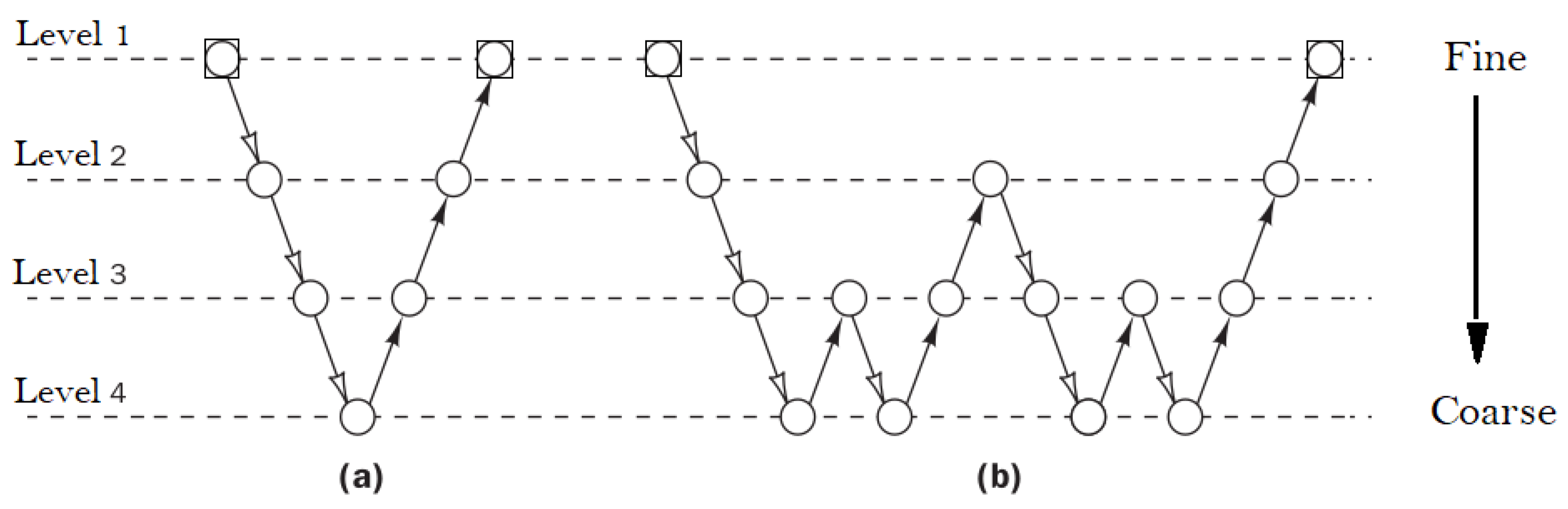
2.5.2. Multigrid Cycles

In our simple example we have illustrated the main concepts of the multigrid methods. In practical CFD calculations, the multigrid transfer process is more sophisticated and different cycles of coarsening and refinement are used with special schedules of restriction and prolongation at different refinement levels. Common choices of multigrid cycles are the so-called V- and W-cycles, which are illustrated in Figure 3.
The simple V-cycle shown in Figure 3a consists of two legs. The calculation starts at the finer level. Iterations at any level are called relaxation. After a few relaxation sweeps on the finer level, the residuals are restricted to the next coarse level, and after relaxation on that level, the residuals are passed on to the next coarse level and so on until the coarsest level is reached. After final relaxation on the coarsest level, the prolongation steps are performed on the upward leg of the V-cycle until the finer level is reached. In the W-cycle, additional restriction and prolongation sweeps are used at coarser levels to obtain a better reduction of long-wavelength errors. A typical pattern is illustrated in Figure 3b.
In general, the multigrid idea requires more than two grids, otherwise its remarkable power would be missed. The lowest frequency errors need to be reduced on a very coarse grid (8 h spacing or higher ) to decay quickly. The two-grid v-cycle can be extended in a natural way to more grids, going down to coarser grids (2 h, 4 h, 8 h, …). As the coarse grid iterations are much faster than fine grid iterations, efficiency may be improved by the decision to switch from one grid to another on the rate of convergence through the combination of V-W cycles. Therefore, the W-cycle, which stays on coarse grids longer, is generally superior to a V-cycle and is used in the present work. Let it be noted that the optimum choice of parameters remains problem-dependent, but their effect on performance is not as dramatic as for the single-grid method.

2.6. Convergence Criteria

Once the solver iteration is completed and the primitive variables corrected, convergence may be monitored by the residual for each of the discretization equations. The discretized equation for general flow variable ϕ at control volume i can be expressed as follows:
( a P ϕ P ) i = n b a n b ϕ n b i + ( b ϕ ) i
The final solution will not satisfy Equation (38) exactly at all cells in the mesh, but after k iterations, there will be a difference between the left and right hand sides. The absolute value of this difference at mesh cell i is termed the local residual ( R ϕ ) i ( k ) :
( R ϕ ) i ( k ) = ( a P ϕ P ) i ( k ) n b a n b ϕ n b i ( k ) ( b ϕ ) i ( k )
To get an indication of the convergence behavior across the whole flow field, we define the global residual R ϕ ( k ) , which is the sum of the local residuals over all N control volumes within the computational domain. After k iterations we have:
R ϕ ( k ) = i = 1 N ( R ϕ ) i ( k ) = i = 1 N ( a P ϕ P ) i ( k ) n b a n b ϕ n b i ( k ) ( b ϕ ) i ( k )
Inspection of Equation (40) shows that the magnitude of the global residual R ϕ decreases as we get closer to the final solution, since the size of the local residuals should decrease in a converging sequence. Thus, it would seem that R ϕ might be a satisfactory single number indicator of convergence. However, the global residual will be larger in simulations where the flow variable ϕ has a larger magnitude, so we would need to specify different truncation values for R ϕ . This can be resolved if we use a global residual that is scaled to take out the magnitude of ϕ . Thus, we define the normalized global residual R ϕ ¯ for flow variable ϕ after k iterations as follows:
R ϕ ¯ ( k ) = R ϕ ( k ) / F R ϕ
where:
F R ϕ = i = 1 N | ( a P ϕ P ) i ( k ) |

2.7. Test Cases

The lid-driven cavity flow is considered by many researchers when testing computational fluid dynamics codes due to the wide range of fluid flow phenomena that can be observed in this simple flow configuration. Thereupon, the effectiveness of the solution procedure developed in this work are first demonstrated for flow in a square cavity of side L, where the top boundary (lid) moves horizontally towards the right with a uniform velocity U, while the remaining sides are fixed. The moving lid, in conjunction with the shear properties of the fluid, lead to a recirculation of the flow in the cavity, see Figure 4.
Next, we assess the method described above on a steady pipe flow test as shown in the schematic diagram of the domain in Figure 5. For this case, the boundary conditions are a steady velocity uniform profile at the inlet and standard no-slip condition at the walls are implemented. The pressure is derived by extrapolation from the inner nodes. Test cases are solved for Reynolds numbers up to R e = 10 3 , and for Bingham numbers up to 200. The flow configuration and the system of coordinates in both cases are shown in Figure 4 and Figure 5.

3. Numerical Results

All the numerical steady-state solutions presented in this section are obtained on Cartesian grids consisting of square control volumes. The Papanastasiou model is employed for the evaluation of viscosity and the stress growth parameter ( m ) is fixed to 200, a sufficiently high value that allows the ideal Bingham behavior to be approximated with satisfactory accuracy. The approximation of the convection terms in the momentum equations is carried out using the Quadratic Upwind Interpolation for the Convective Kinematics (QUICK) scheme.
In the present study, Reynolds number ( R e ) and Bingham number ( B n ) are taken as independent parameters. These two numbers are defined as follows:
R e = ρ U L μ p
B n = τ y L μ p U
with zero yield stress ( B n = 0 ) in case of Newtonian fluid. The Bingham number standing for the ratio of yield stress to viscous force is a crucial dimensionless number to describe viscoplastic materials.

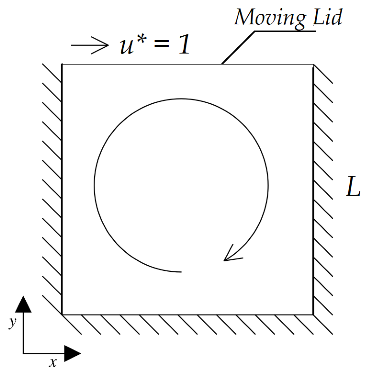
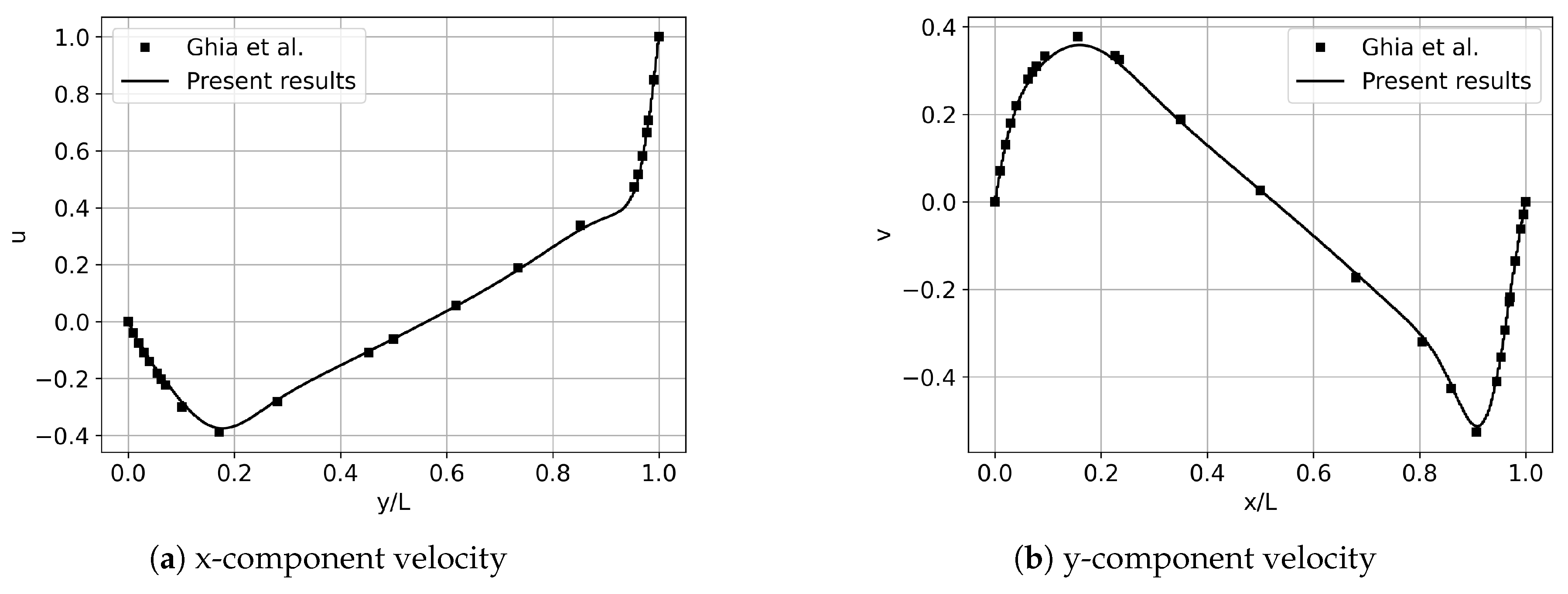
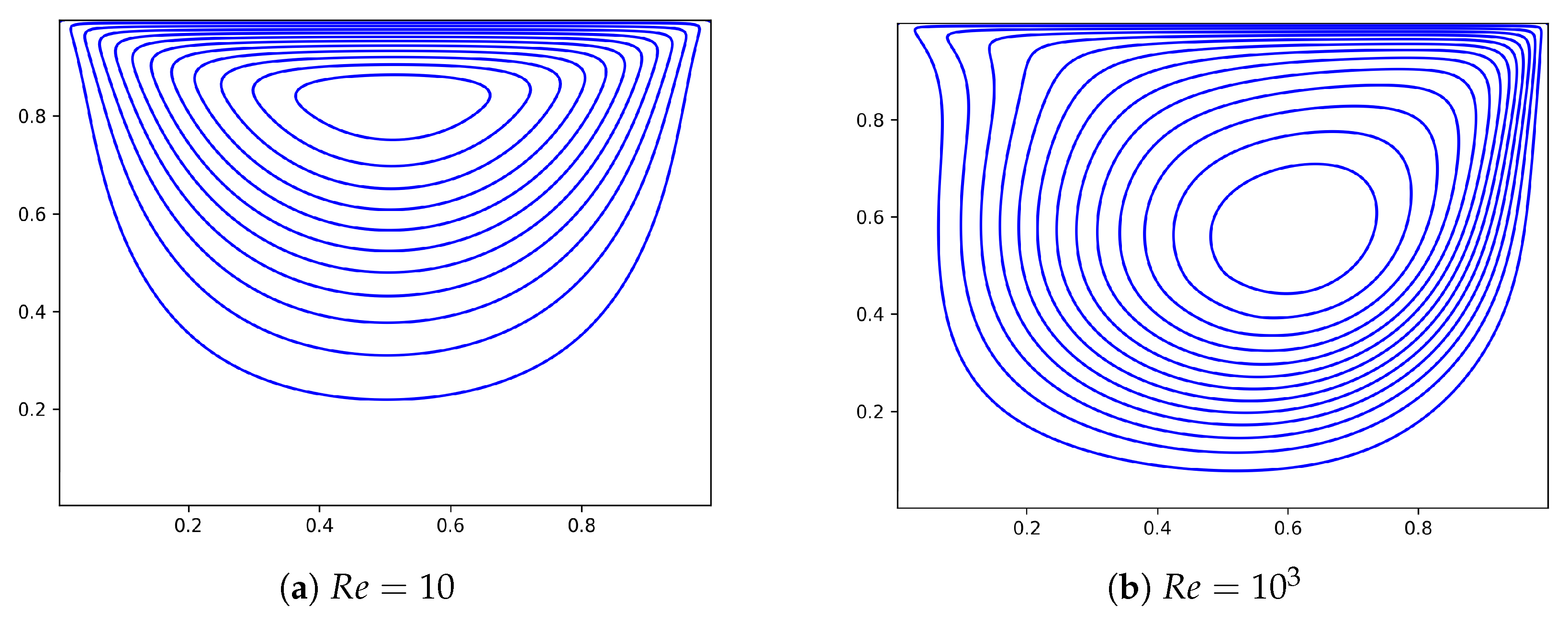
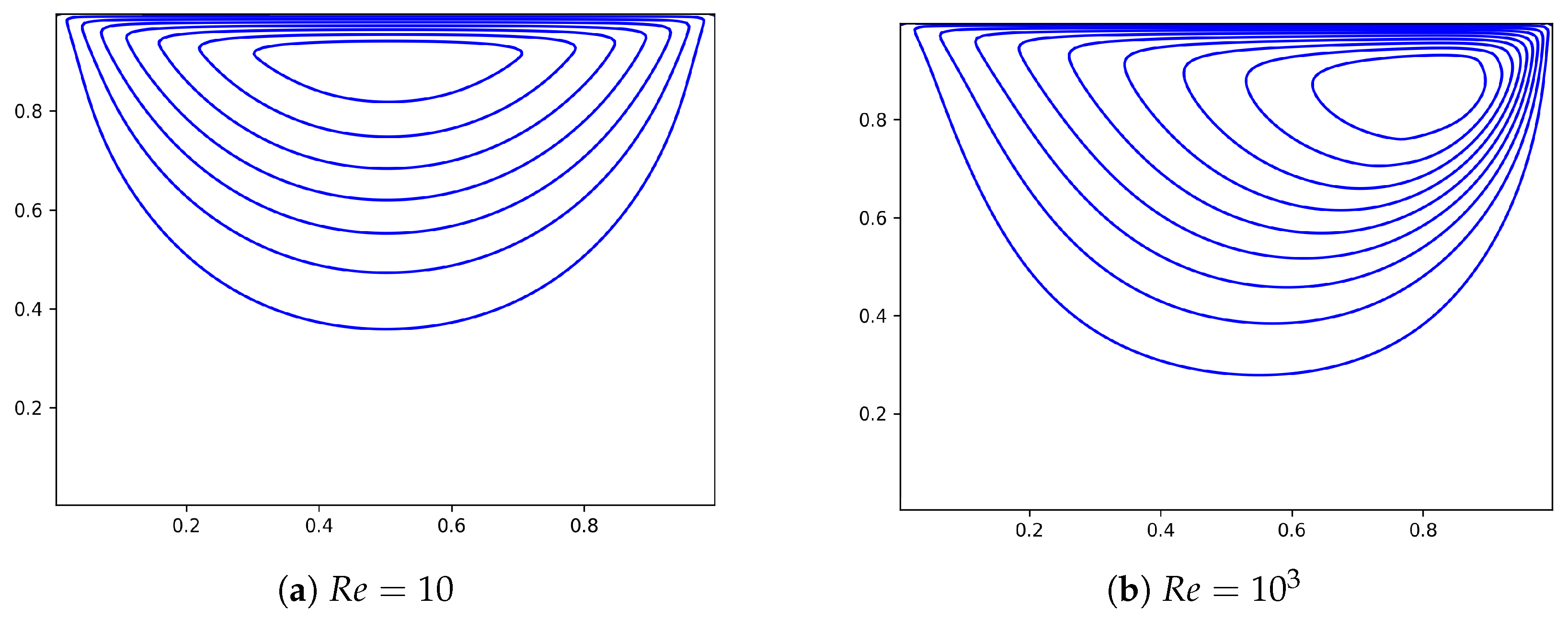
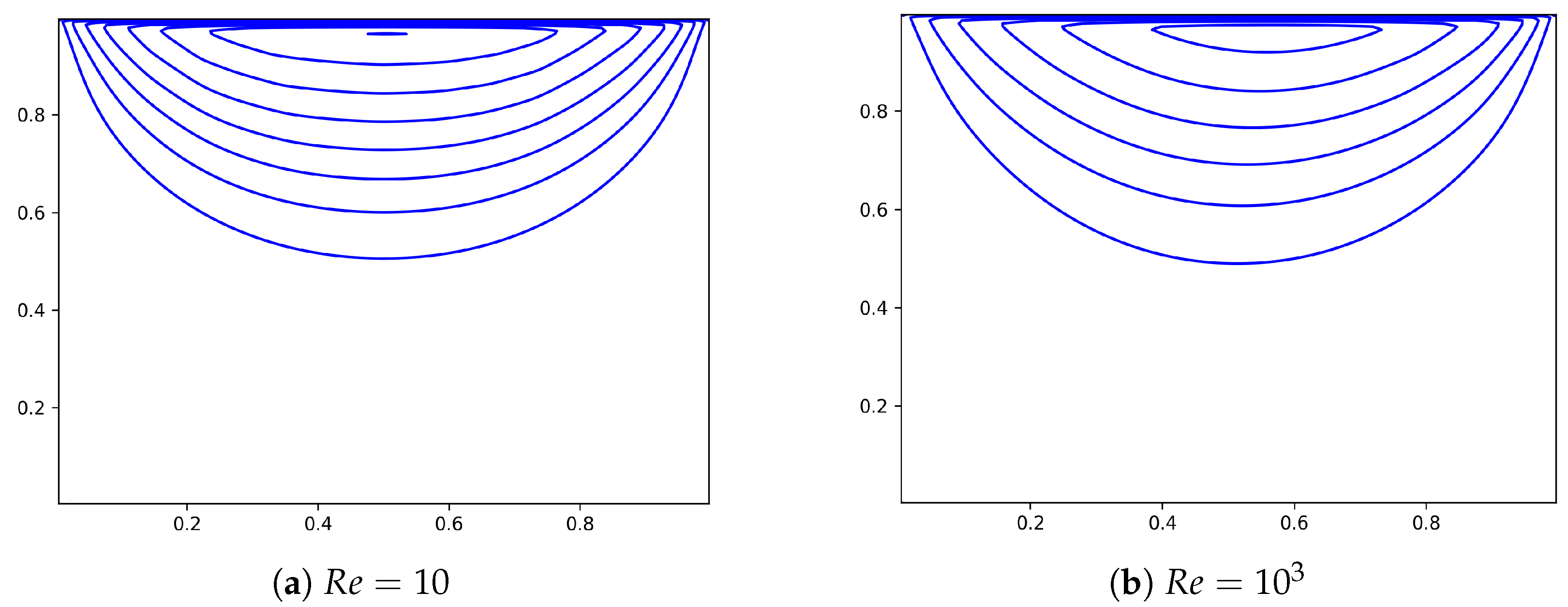
3.1. Verification of the Numerical Method: Lid Driven Cavity

We now turn our attention to validating the numerical results obtained using the Simple/regularization procedure of our code. To this end, we consider the test case of lid-cavity flow, which is the prototypical recirculation flow and has long been used as a standard problem for testing and evaluating Navier–Stokes solvers. Many authors provided high quality benchmark results for this particular problem, most famous of which are Ghia et al. [36] who used a coupled strongly implicit multigrid (CSI-MG) in a uniform mesh of 257 × 257. They presented a second-order accurate results that have served as “The” result for Newtonian flows to compare against ever since.
All the results presented in this section are obtained on Cartesian grids consisting of 320 × 320 square control volumes. To validate the present algorithm, first, a Newtonian flow ( B n = 0 ) in the R e = 10 3 case is calculated. Figure 6a,b show the evolution of the horizontal and vertical velocities along the mid-planes x = 0.5 and y = 0.5 , with the corresponding numerical result of Ghia et al. [36]. The present results are in good agreement with those numerical data.
Now we consider the steady viscoplastic flow at various Bingham numbers (Bn) in the case of R e = 10 3 . For this particular flow, many of the previous studies (Mitsoulis et al. [12]; Vola et al. [37]; Prashant et al. [38]; Syrakos et al. [23]) formulated the main quantitative results in terms of the features of the flow vortices. To this end, we need to calculate the stream function on the whole domain through integration of the velocity field ( u = ψ / y , v = ψ / x ). The location of the primary vortex formed in lid-driven cavity flow is significantly influenced by both Bingham and Reynolds numbers. This shifting of location is easily noticeable, which allows us to further assess the qualitative aspect of the simulation results. The evolution of the center position of the principal vortex is compared to the results of the predictions performed by Vola et al. [37] and Prashant et al. [38], with a regularized constitutive law on Figure 7. The obtained values once again compare fairly well with the literature, indicating that the treatment of the shear stress and viscosity in the non-Newtonian flow prediction is feasible and the steady SIMPLE solver for Bingham fluid is correct.
The evolution of the principal vortex location as a function of the yield stress drawn in Figure 7 shows that the primary vortex goes up toward the moving lid as B n increases. Increasing the yield stress leads to restricting the flow region closer to the upper moving boundary due to the resistance to lid motion, which gets higher. In viscoplastic flows, rigid zones are located at the bottom of the cavity where the shear stresses are very low as the fluid in contact is motionless due to the no-slip boundary condition. These unyielded regions expand significantly with the increase of the Bingham number, leading the main vortex to move toward the upper boundary as there is less space for flow to happen. The streamline contour evolution shown in Figure 8, Figure 9 and Figure 10 highlights the progressive growth of the unyielded zones. At constant R e number, as the value of the Bingham number increases, the main vortex center gets closer to the upper cavity side and the zone sheared by the upper boundary becomes thinner.
Figure 8, Figure 9 and Figure 10 display the flow field as the bingham number increases, for R e = 10 and R e = 10 3 , respectively. When R e = 10 , the streamline contours are symmetric for all Bingham numbers, 2, 10, and 100. However, the unyielded zone is proportional to the yield stress magnitude. At R e = 10 3 , the primary vortex shifts slightly to the right for the case of B n = 100 , and moves further in the same direction for B n = 10 , then towards the center of the cavity for B n = 2 . We see that increasing the Reynolds number moves the vortex first toward the right, and then downwards and left to the center depending on the value of the Bingham number. This trend can be observed for higher Bingham numbers if the Reynolds number is large enough as greater stresses are required in order to make the material flow. In the works of [23,38], similar conclusions were drawn, the flow field at high Bn numbers follow the same trend of any lower Bn number if the Re number is also sufficiently decreased.

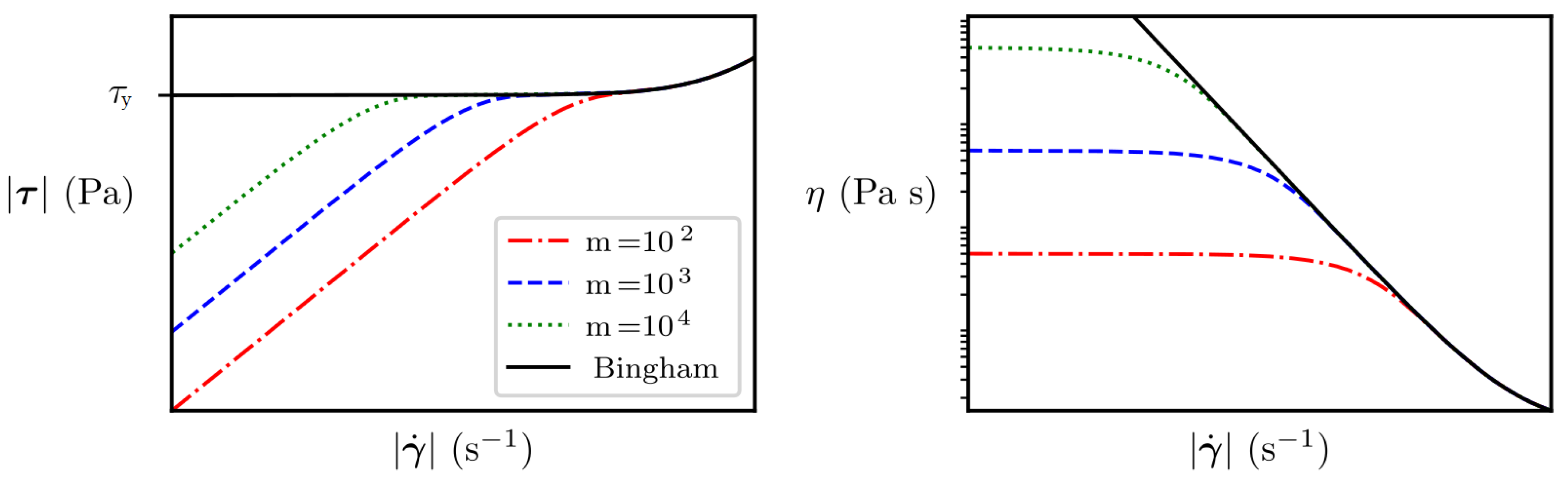
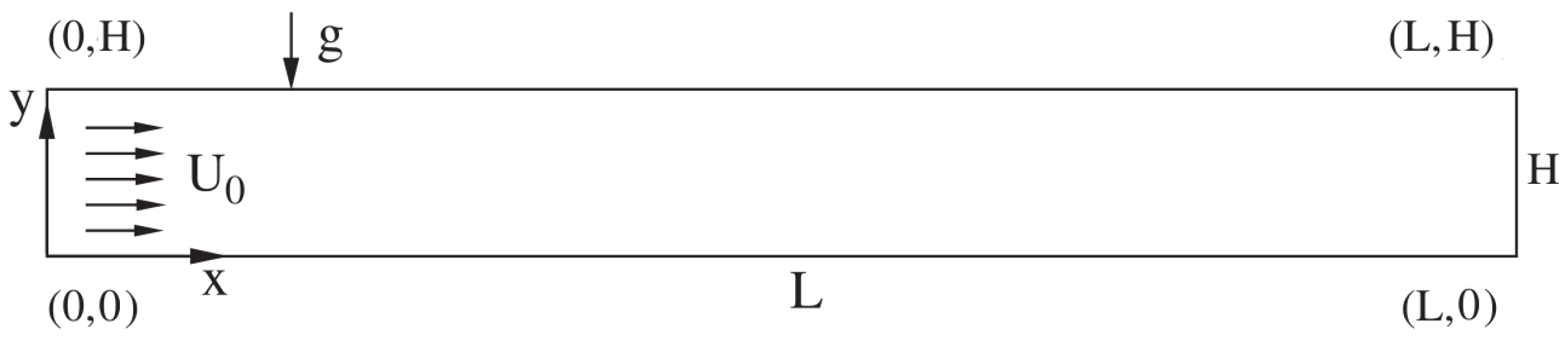
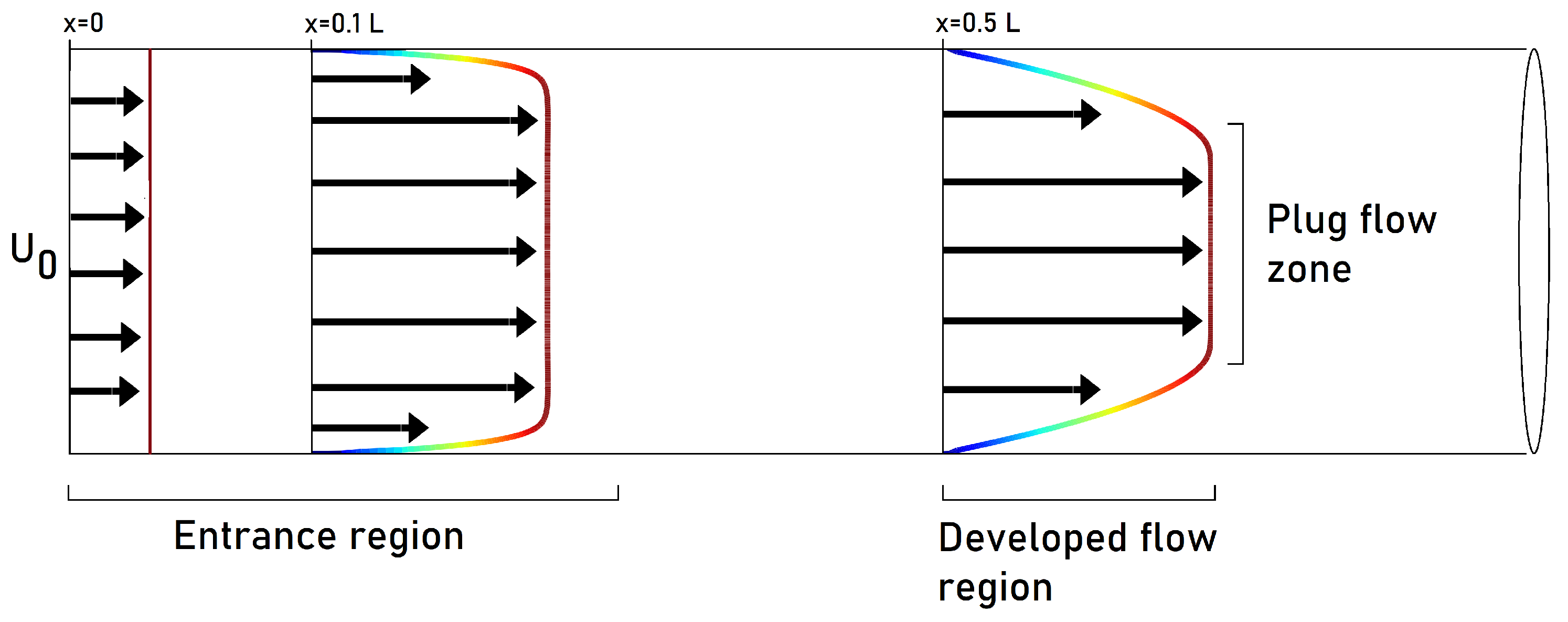
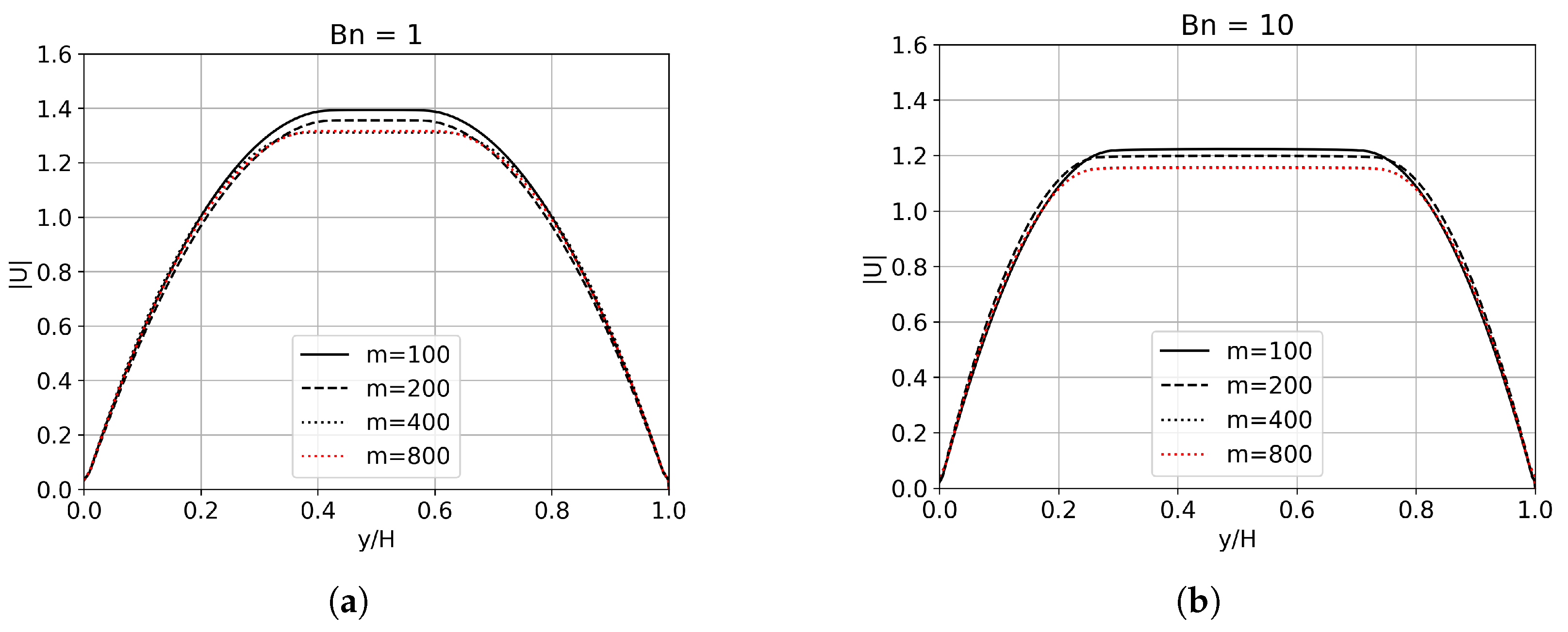
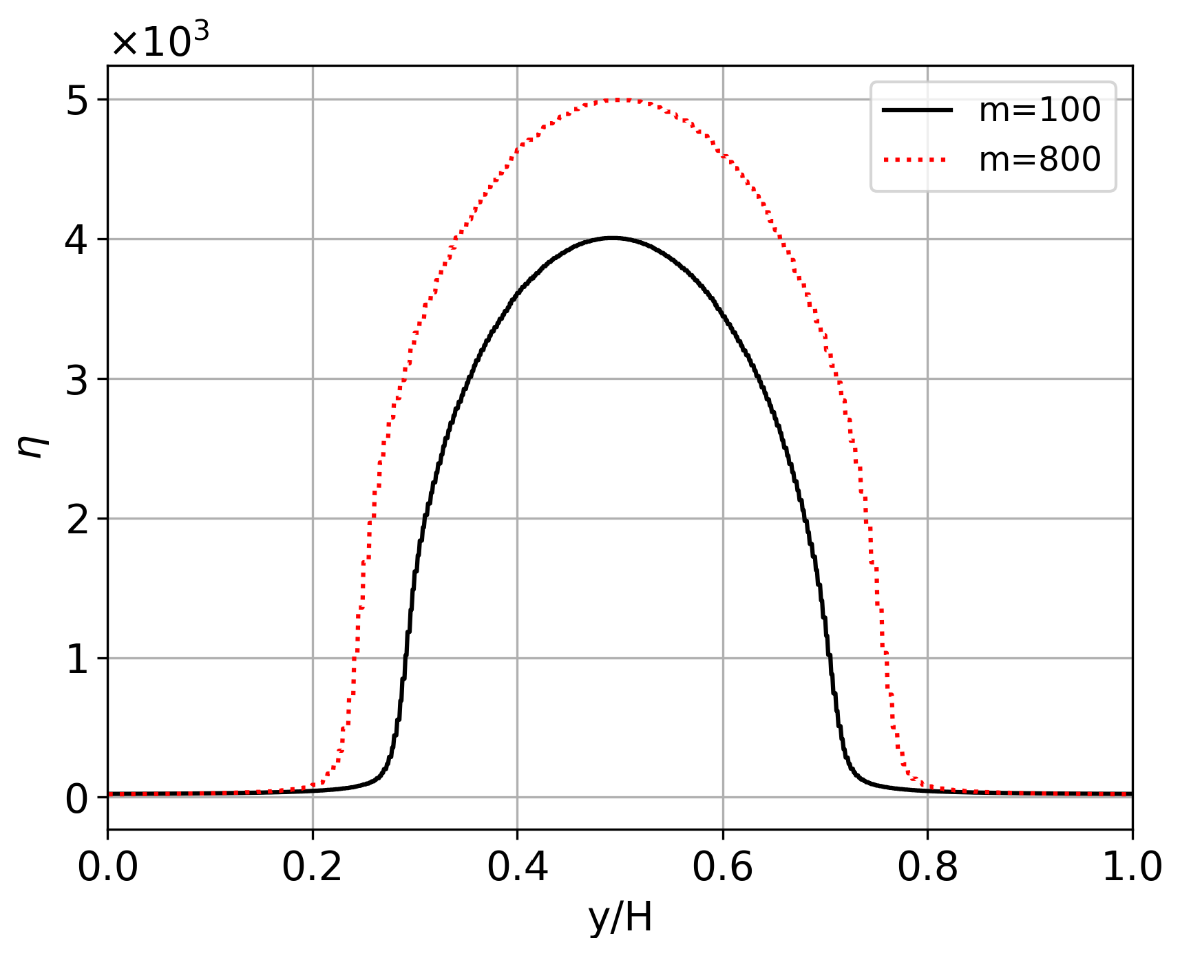
3.2. Influence of the Stress Growth Parameter: Pipe Flow

The results of Equation (10) are plotted in Figure 1 with dashed lines, along with the the actual Bingham constitutive equation, τ = ( μ + τ y / | γ ˙ | ) γ ˙ . It is clear that with an increasing exponent m, we can achieve quick stress growth at very low shear rates, which is consistent with the behavior of the material in its unyielded region. In fact, regularized models yield results that do not contain truly unyielded or solid zones and hence the solution may, in some cases, be sensitive to the chosen stress growth exponent. Previous studies, including [10], found that different values of 100, 200, and 400 for m do not influence the location of the yield surface significantly, for the particular case of cavity flow. However, very large values of the exponent parameter may be needed if the region where the stress close to the yield stress is relatively large.
Regarding the viscoplastic flows though pipes, two distinct unyielded regions can possibly occur. First, in the layer adjacent to no-slip boundary where the velocity of the fluid is set to zero, it is called the stagnant zone. Then, a second unyielded region with non-zero fluid velocity is referred to as the plug zone, see Figure 11. One result of importance in a range of applications is the location of the plug zone, where | γ ˙ | tends to zero, as previously stated. In Figure 12, we present a comparison of the velocity profiles for different values of m: 100, 200, 400, and 800. As m is increased, the location of the unyielded region would be slightly affected. The difference especially vanished between m = 400 and m = 800 for both cases. Figure 12 shows velocity profiles, which deviate slightly from the reference result considered here in red dotted lines ( m = 800 ) and plug zones which get flatter as m is increased. Indeed, beyond a certain value of stress growth exponent, yield lines ( τ = τ y ) are less sensitive to its variation. This verifies the assumption that the yield areas calculated using a regularization approach will converge to the true yield areas as m . It should be pointed out that, unlike the velocity field, there is no theoretical proof that yield surfaces converge to the exact solution [11].
In Figure 13, we compare the simulated results of the apparent viscosity profiles along the circular cross-section of the pipe calculated with m = 100 and m = 800 . It is shown that using a high value of the exponent m leads to fast growing apparent viscosity as the shear rates are decreasing, meaning that the larger the value of m, the larger the region of the solid-like behavior of the Bingham model is reproduced. Figure 13 also shows that, with regularized models, the unyielded material (plug zone) is no longer a rigid solid but a highly viscous fluid that approximates the ideal viscoplastic behavior. The degree of approximation depends on the adequate choice of the stress growth parameter in order to satisfy the von Mises criterion.
An important issue when using the Papanastasiou regularization is that the degree of non linearity increass sharply with higher values of m that ensure better approximations. Therefore, as a matter of practicality, the choice of exponent m has to be reasonably reduced depending on the problem under study. In this work, we limited our study to the comparisons showing the influence of m on the quality of the results. The reader may refer to the interesting assessments provided by Syrakos et al. [10] and Frigaard et al. [11] on the issues of feasibility and the computational effort required as a function of the stress growth exponent. They suggested that, in some cases, to achieve a fully-converged solution with a high value of m, one can start with a very low value of m as an initial guess, and progressively increase it every certain number of SIMPLE iterations.

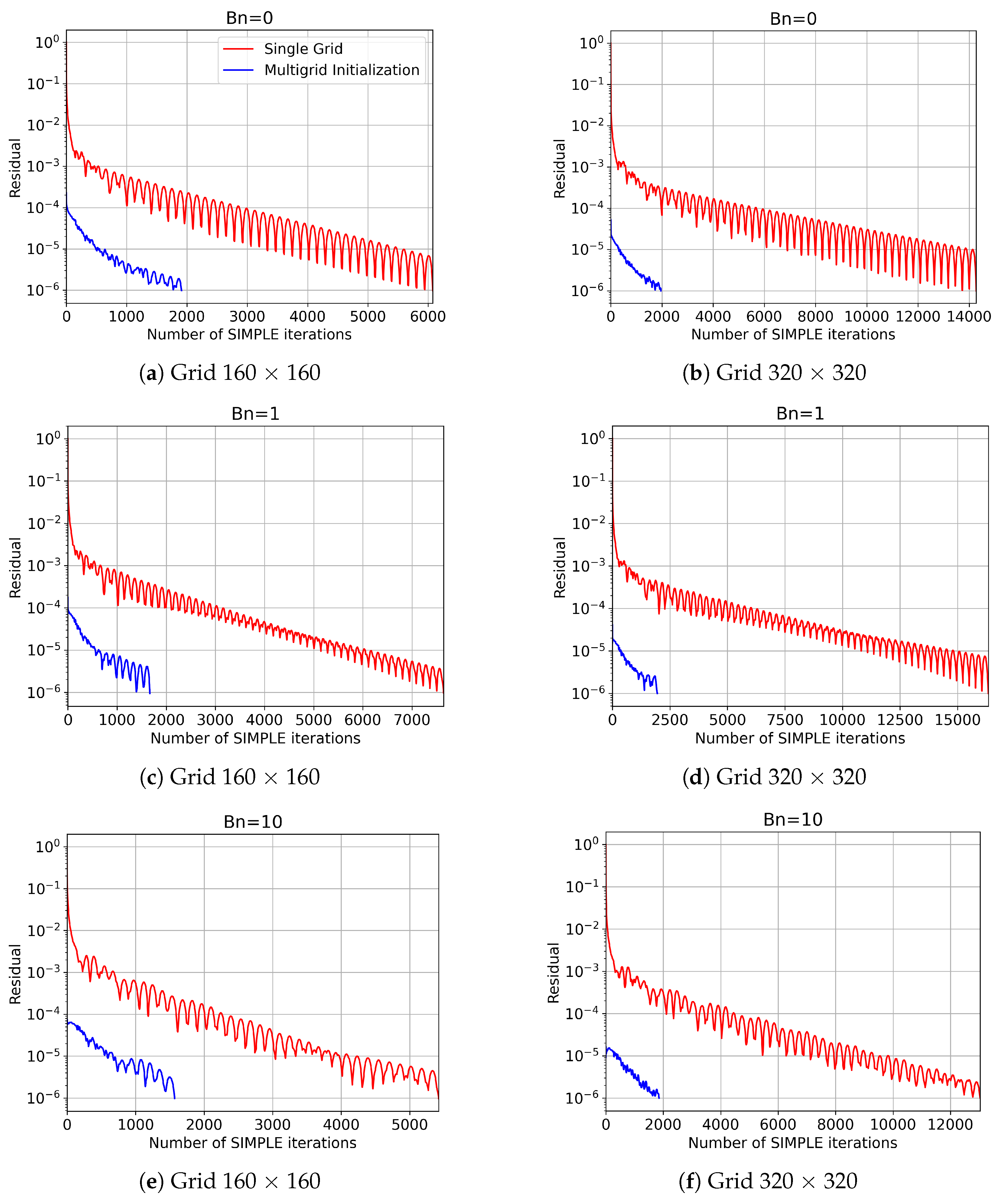
3.3. Algebraic Convergence of the SIMPLE/Regularization Procedure

In viscoplastic flows, derivatives of the flow variables take significantly higher values across the yield surfaces in the limit between the unyielded and yielded regions. This disparity is due to the fact that these derivatives are zero inside the rigid zones and non-zero outside. In addition, increasing the Bingham number and growth stress parameter would further widen this gap. As a result, solution errors are found to be much larger there than the rest of the domain, causing inefficiencies and deterioration in convergence rates of iterative solvers. In such cases, using fine grids can considerably reduce the numerical errors and address more efficiently the high values of the derivatives. However, it is well known that the number of iterations required for convergence increases almost linearly with the number of control volumes for the single grid set [19,27]. To address this limitation, one may notice that using an appropriate initial solution is very important for fine grids and contributes to the enhancement of the convergence of iterative solvers. To this end, a steady lid driven cavity flow simulation is carried out for different Bingham numbers 0, 1, and 10 at R e = 10 2 using single-grid (SG) and multi-grid (MG) initialization methods.
Figure 14 demonstrates the convergence of the L norm of u and v residuals as a function of the number of SIMPLE iterations on the finer grids. It shows that the performance of SIMPLE, as a single-grid solver, deteriorates, and more iterations are needed as the number of control volumes increases for all cases. In contrast, computations with MG initialization exhibit near constant number for both 160 × 160 and 320 × 320 grids. In all cases, the number of iterations has drastically been reduced compared to the single grid computation. One may also observe that convergence becomes faster in the case of B n = 10 , but it also becomes more unstable and oscillatory. It should be noted that for higher Bingham numbers, convergence difficulties may be encountered. In order to overcome this difficulty, low under-relaxation factors for pressure and velocity field, denoted by α p , α u , and α v can be considered within the numerical solver [10]. This technique was found to be efficient in making the solver more robust, but we observed that it leads to a slow down in convergence rate. Another remedy to this problem could be the suggestion of Ferziger and Peric [19] in a multigrid context. They recommend updating the viscosity on the finer grid only and holding its value constant on coarse grids within the multigrid cycle.
The performance of multi-grid (MG) initialization is based on the speedup characteristics, and a comparison between the number of iterations and computation times, as summarized in Table 1. In all cases, CPU time is recorded until the convergence of residuals is achieved. In the case of MG Initialization, the total simulation time includes computation time on both multilevel grids during initialization, and the finer grid, which is the true representation of the simulation time. The simulations are performed on a Core i7-6700HQ CPU @ 2.60GHz × 8, 8 GB RAM-based computer. According to our numerical experiments, the speed-up ratio between single grid and multigrid initialization methods is around 6 for 320 × 320 grids and up to 3 for 160 × 160 grids. This confirms the potential of multigrid initialization technique for improving the convergence over single-grid method by significantly reducing CPU time and number of iterations. Since MG initialization does most of the computations on coarse grids, this initialization procedure is computationally inexpensive and, for very dense grids, a good initial solution can be obtained in a fraction of the time spent to converge on a final solution. The computational effort can be further reduced when parallel algorithms and high performance computing machines are used [24].

4. Conclusions

This paper introduced the idea of multigrid initialization to overcome the drawbacks of solvers using single grids for viscoplastic flows. The proposed solver is easy to implement and significantly improves the convergence rate by reducing CPU time and number of iterations. The computational procedure employed in this work is based on the finite volume / SIMPLE algorithm in conjunction with the regularization scheme of Papanastasiou and is applied for the solution of the lid-driven cavity and pipe flow problems. The convection terms are discretized using the QUICK scheme in order to avoid any artificial diffusion that may be caused by interpolation schemes of low order of accuracy. The capability of the algorithm for solving viscoplastic flows was verified against a number of benchmark solutions for a range of Bingham numbers in the case of lid-driven cavity flow. A qualitative assessment was also conducted by monitoring the positioning of the principal vortex with regard to Bingham and Reynolds numbers. Results from the current study were accurate and compare favorably with the published results. In order to analyze the influence of the growth stress parameter ( m ) of the regularization model on fluid motion, pipe flow tests for different values of ( m ) and B n were considered. Numerical simulations confirmed that a large value of m reproduced a large threshold-like region. The result also showed that as m increases, the yield surface converges to the true yield region, with no significant influence beyond a value of 400 in this particular case. Furthermore, the results clearly reveal that introducing the multigrid method as an initialization procedure yields better convergence for Navier–Stokes equations for viscoplastic flows compared to the single-grid method. A multi-grid initialization speed-up ratio as high as 6.45 was achieved for the finest grid size (320 × 320).
The present study can be extended to the numerical solution of non-Newtonian problems with a different definition of effective viscosity and accounting for complex geometries encountered in many industrial processes. This part is the subject of an ongoing investigation that is to be published in our future works.

Author Contributions

Conceptualization, S.M. and I.K.; methodology, S.M., I.K. and F.B.; validation, S.M., I.K. and F.B.; formal analysis, S.M. and F.B.; investigation, S.M., I.K., D.O. and F.B.; data curation, S.M.; writing—original draft preparation, S.M.; writing—review and editing, S.M., I.K. and F.B.; visualization, F.B.; supervision, I.K., D.O. and F.B.; project administration, D.O. and F.B. All authors have read and agreed to the published version of the manuscript.

Funding

This research received no external funding.

Data Availability Statement

The data presented in this study are available on request from the corresponding author.

Acknowledgments

The authors gratefully acknowledge the support and computing resources from the African Supercomputing Center (ASCC) at UM6P (Morocco).

Conflicts of Interest

The authors declare no conflict of interest. The funders had no role in the design of the study; in the collection, analyses, or interpretation of data; in the writing of the manuscript; in the decision to publish the results.

References

  1. Apostolidis, A.J.; Beris, A.N. Modeling of the blood rheology in steady-state shear flows. J. Rheol. 2014, 58, 607–633. [Google Scholar] [CrossRef]
  2. Frigaard, I.A.; Paso, K.G.; de Souza Mendes, P.R. Bingham’s model in the oil and gas industry. Rheol. Acta 2017, 56, 259–282. [Google Scholar] [CrossRef] [Green Version]
  3. Akhtar, S.; Almutairi, S.; Nadeem, S. Impact of heat and mass transfer on the Peristaltic flow of non-Newtonian Casson fluid inside an elliptic conduit: Exact solutions through novel technique. Chin. J. Phys. 2022, 78, 194–206. [Google Scholar] [CrossRef]
  4. Akbar, N.S.; Akhtar, S. Metachronal wave form analysis on cilia-driven flow of non-Newtonain Phan–Thien–Tanner fluid model: A physiological mathematical model. Proc. Inst. Mech. Eng. Part E J. Process Mech. Eng. 2022, 09544089221140703. [Google Scholar] [CrossRef]
  5. Barnes, H.A. The yield stress—A review or ‘παντα ρει’—Everything flows? J. Non-Newton. Fluid Mech. 1999, 81, 133–178. [Google Scholar] [CrossRef]
  6. Bingham, E.C. An Investigation of the Laws of Plastic Flow; Number 278; US Government Printing Office: Washington, DC, USA, 1917.
  7. Bercovier, M.; Engelman, M. A finite-element method for incompressible non-Newtonian flows. J. Comput. Phys. 1980, 36, 313–326. [Google Scholar] [CrossRef]
  8. Papanastasiou, T.C. Flows of Materials with Yield. J. Rheol. 1987, 31, 385–404. [Google Scholar] [CrossRef]
  9. Tang, G.; Wang, S.; Ye, P.; Tao, W. Bingham fluid simulation with the incompressible lattice Boltzmann model. J. Non-Newton. Fluid Mech. 2011, 166, 145–151. [Google Scholar] [CrossRef]
  10. Syrakos, A.; Georgiou, G.C.; Alexandrou, A.N. Performance of the finite volume method in solving regularised Bingham flows: Inertia effects in the lid-driven cavity flow. J. Non-Newton. Fluid Mech. 2014, 208–209, 88–107. [Google Scholar] [CrossRef] [Green Version]
  11. Frigaard, I.; Nouar, C. On the usage of viscosity regularisation methods for visco-plastic fluid flow computation. J. Non-Newton. Fluid Mech. 2005, 127, 1–26. [Google Scholar] [CrossRef]
  12. Mitsoulis, E.; Zisis, T. Flow of Bingham plastics in a lid-driven square cavity. J. Non-Newton. Fluid Mech. 2001, 101, 173–180. [Google Scholar] [CrossRef]
  13. Sverdrup, K.; Nikiforakis, N.; Almgren, A. Highly parallelisable simulations of time-dependent viscoplastic fluid flow with structured adaptive mesh refinement. Phys. Fluids 2018, 30, 093102. [Google Scholar] [CrossRef] [Green Version]
  14. Busto, S.; Dumbser, M.; Río-Martín, L. Staggered Semi-Implicit Hybrid Finite Volume/Finite Element Schemes for Turbulent and Non-Newtonian Flows. Mathematics 2021, 9, 2972. [Google Scholar] [CrossRef]
  15. Duvaut, G.; Lions, J.L. Rigid visco-plastic Bingham fluid. In Inequalities in Mechanics and Physics; Grundlehren der Mathematischen Wissenschaften; Springer: Berlin/Heidelberg, Germany, 1976; Volume 219, pp. 278–327. [Google Scholar]
  16. Glowinski, R. Sur L’Ecoulement D’Un Fluide De Bingham Dans Une Conduite Cylindrique. J. MéCanique 1974, 13, 601–621. [Google Scholar]
  17. Saramito, P.; Wachs, A. Progress in numerical simulation of yield stress fluid flows. Rheol. Acta 2017, 56, 211–230. [Google Scholar] [CrossRef] [Green Version]
  18. Patankar, S.V. Numerical Heat Transfer and Fluid Flow; CRC Press: Boca Raton, FL, USA, 2018. [Google Scholar]
  19. Ferziger, J.H.; Perić, M.; Street, R.L. Computational Methods for Fluid Dynamics; Springer: Berlin, Germany, 2002; Volume 3. [Google Scholar]
  20. Patankar, S.; Spalding, D. A calculation procedure for heat, mass and momentum transfer in three-dimensional parabolic flows. Int. J. Heat Mass Transf. 1972, 15, 1787–1806. [Google Scholar] [CrossRef]
  21. Denner, F.; Evrard, F.; van Wachem, B.G. Conservative finite-volume framework and pressure-based algorithm for flows of incompressible, ideal-gas and real-gas fluids at all speeds. J. Comput. Phys. 2020, 409, 109348. [Google Scholar] [CrossRef] [Green Version]
  22. Versteeg, H.K.; Malalasekera, W. An Introduction to Computational Fluid Dynamics: The Finite Volume Method; Pearson Education: Harlow, UK, 2007. [Google Scholar]
  23. Syrakos, A.; Georgiou, G.C.; Alexandrou, A.N. Solution of the square lid-driven cavity flow of a Bingham plastic using the finite volume method. J. Non-Newton. Fluid Mech. 2013, 195, 19–31. [Google Scholar] [CrossRef] [Green Version]
  24. Roy, P.; Anand, N.K.; Donzis, D. A Parallel Multigrid Finite-Volume Solver on a Collocated Grid for Incompressible Navier-Stokes Equations. Numer. Heat Transf. Part B Fundam. 2015, 67, 376–409. [Google Scholar] [CrossRef]
  25. Tong, Z.X.; He, Y.L.; Tao, W.Q. A review of current progress in multiscale simulations for fluid flow and heat transfer problems: The frameworks, coupling techniques and future perspectives. Int. J. Heat Mass Transf. 2019, 137, 1263–1289. [Google Scholar] [CrossRef]
  26. Sivaloganathan, S.; Shaw, G.J. A multigrid method for recirculating flows. Int. J. Numer. Methods Fluids 1988, 8, 417–440. [Google Scholar] [CrossRef]
  27. Peric, M.; Rüger, M.; Scheuerer, G. A finite volume multigrid method for calculating turbulent flows. In Proceedings of the 7th Symposium on Turbulent Shear Flows, Stanford, CA, USA, 21–23 August 1989; Volume 1, pp. 3–7. [Google Scholar]
  28. Zhang, C.; Tan, J.; Ning, D. Machine learning strategy for viscous calibration of fully-nonlinear liquid sloshing simulation in FLNG tanks. Appl. Ocean Res. 2021, 114, 102737. [Google Scholar] [CrossRef]
  29. Saghi, R.; Hirdaris, S.; Saghi, H. The influence of flexible fluid structure interactions on sway induced tank sloshing dynamics. Eng. Anal. Bound. Elem. 2021, 131, 206–217. [Google Scholar] [CrossRef]
  30. Vångö, M.; Pirker, S.; Lichtenegger, T. Unresolved CFD–DEM modeling of multiphase flow in densely packed particle beds. Appl. Math. Model. 2018, 56, 501–516. [Google Scholar] [CrossRef]
  31. Giussani, F.; Piscaglia, F.; Sáez-Mischlich, G.; Hèlie, J. A three-phase VOF solver for the simulation of in-nozzle cavitation effects on liquid atomization. J. Comput. Phys. 2020, 406, 109068. [Google Scholar] [CrossRef]
  32. Di Iorio, S.; Catapano, F.; Magno, A.; Sementa, P.; Vaglieco, B.M. Investigation on sub-23 nm particles and their volatile organic fraction (VOF) in PFI/DI spark ignition engine fueled with gasoline, ethanol and a 30% v/v ethanol blend. J. Aerosol Sci. 2021, 153, 105723. [Google Scholar] [CrossRef]
  33. Hayase, T.; Humphrey, J.A.; Greif, R. A consistently formulated QUICK scheme for fast and stable convergence using finite-volume iterative calculation procedures. J. Comput. Phys. 1992, 98, 108–118. [Google Scholar] [CrossRef]
  34. Bartholomew, P.; Denner, F.; Abdol-Azis, M.H.; Marquis, A.; van Wachem, B.G. Unified formulation of the momentum-weighted interpolation for collocated variable arrangements. J. Comput. Phys. 2018, 375, 177–208. [Google Scholar] [CrossRef]
  35. Rhie, C.M.; Chow, W.L. Numerical study of the turbulent flow past an airfoil with trailing edge separation. AIAA J. 1983, 21, 1525–1532. [Google Scholar] [CrossRef]
  36. Ghia, U.; Ghia, K.; Shin, C. High-Re solutions for incompressible flow using the Navier-Stokes equations and a multigrid method. J. Comput. Phys. 1982, 48, 387–411. [Google Scholar] [CrossRef]
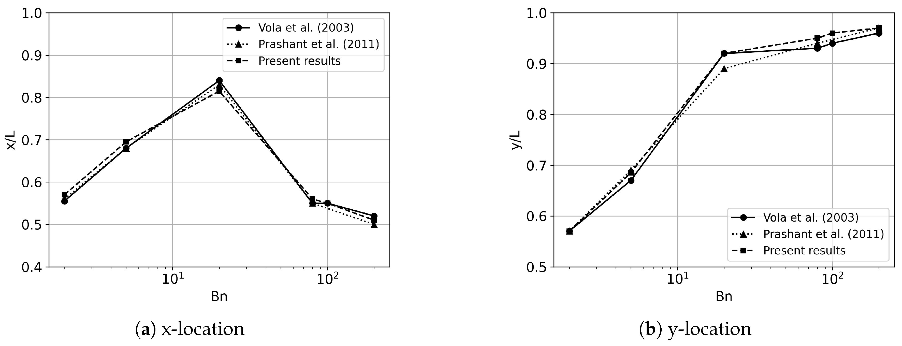
  37. Vola, D.; Boscardin, L.; Latché, J. Laminar unsteady flows of Bingham fluids: A numerical strategy and some benchmark results. J. Comput. Phys. 2003, 187, 441–456. [Google Scholar] [CrossRef]
  38. Prashant; Derksen, J. Direct simulations of spherical particle motion in Bingham liquids. Comput. Chem. Eng. 2011, 35, 1200–1214. [Google Scholar] [CrossRef]
Figure 1. Papanastasiou regularization for the Bingham model: stress magnitude (left) and apparent viscosity (right) as functions of the magnitude of the shear rate tensor γ ˙ .
Algorithms 16 00050 g001
Figure 2. Two-dimensional orthogonal grid. N, S, E and W correspond to neighbor cells of cell P; n, s, e and w denote cell P faces; Δ x and Δ y are cell P dimensions in the x and y spatial coordinates; δ y n , δ y s , δ x e and δ x w correspond to cell-center to cell-center distances from cell P to neighbor cells.
Algorithms 16 00050 g002
Figure 3. Illustration of different multigrid cycle strategies: (a) V-cycle, (b) W-cycle.
Algorithms 16 00050 g003
Figure 4. Geometry of a cavity with moving lid.
Algorithms 16 00050 g004
Figure 5. Geometry of a two-dimensional pipe of circular cross-section. Dimensions are height H and length L.
Algorithms 16 00050 g005
Figure 6. Sections of velocity along the vertical (a) and horizontal (b) mid-planes, R e = 10 3 [36].
Algorithms 16 00050 g006
Figure 7. Principal vortex position for various B n numbers at R e = 10 3 . Reference results retrieved from Vola et al. [37] and Prashant et al. [38].
Algorithms 16 00050 g007
Figure 8. Streamline contours in Bingham flow for B n = 2 .
Algorithms 16 00050 g008
Figure 9. Streamline contours in Bingham flow for B n = 10 .
Algorithms 16 00050 g009
Figure 10. Streamline contours in Bingham flow for B n = 100 .
Algorithms 16 00050 g010
Figure 11. Numerical results: the developing velocity profile of a Bingham fluid entering the pipe, R e = 10 2 and B n = 10 .
Algorithms 16 00050 g011
Figure 12. Velocity profiles at x = 0.5   L calculated with m = 100 (solid lines), m = 200 (dashed lines), m = 400 (dotted lines), and m = 800 (red dotted lines). For R e = 10 2 , (a) B n = 1 , and (b) B n = 10 .
Algorithms 16 00050 g012
Figure 13. Apparent viscosity profiles along the vertical section x = 0.5   L calculated with m = 100 (solid lines) and m = 800 (red dotted lines), R e = 10 2 and B n = 10 .
Algorithms 16 00050 g013
Figure 14. The L norm of u and v residuals as a function of the number of SIMPLE iterations on the fine grid, for B n = 0 , 1, and 10 ( R e = 10 2 ). Results are shown for simulations with single-grid (SG) in red lines and multi-grid (MG) initialization in blue lines.
Algorithms 16 00050 g014
Table 1. MG Initialization performance for different Bingham numbers.
Bingham NumberNumber of CellsCPU Time (s)Number of IterationsSpeed-Up Ratio
Single GridMG InitializationSingle GridMG Initialization
0160 × 16088.235.8607619102.46
320 × 320872.9143.714,27219646.07
1160 × 160109.932.4764316703.39
320 × 320990.1153.416,33719566.45
10160 × 16081.629.8542415692.73
320 × 320797.3141.513,03318565.63
Disclaimer/Publisher’s Note: The statements, opinions and data contained in all publications are solely those of the individual author(s) and contributor(s) and not of MDPI and/or the editor(s). MDPI and/or the editor(s) disclaim responsibility for any injury to people or property resulting from any ideas, methods, instructions or products referred to in the content.

