Three Diverse Applications of General-Purpose Parameter Optimization Algorithm

Abstract

Parameters often take key roles in determining the accuracy of algorithms, logics, and models for practical applications. Previously, we have proposed a general-purpose parameter optimization algorithm, and studied its applications in various practical problems. This algorithm optimizes the parameter values by repeating small changes of them based on a local search method with hill-climbing capabilities. In this paper, we present three diverse applications of this algorithm to show the versatility and effectiveness. The first application is the fingerprint-based indoor localization system using IEEE802.15.4 devices called FILS15.4 that can detect the location of a user in an indoor environment. It is shown that the number of fingerprints for each detection point, the fingerprint values, and the detection interval are optimized together, and the average detection accuracy exceeds $99\%$. The second application is the human face contour approximation model that is described by a combination of half circles, line segments, and a quadratic curve. It is shown that the simple functions can well approximate the face contour of various persons by optimizing the center coordinates, radii, and coefficients. The third application is the computational fluid dynamic (CFD) simulation to estimate temperature changes in a room. It is shown that the thermal conductivity is optimized to make the average temperature difference between the estimated and measured $0.22$${}^{\circ }$C.

1. Introduction

Parameters often take key roles in determining the accuracy and efficiency of algorithms, logic, and models for practical applications. Some parameters are sensitive to influence the program running efficiency, the calculation results, and the estimation accuracies of them. Therefore, the values of such sensitive parameters should be properly selected before running the programs for algorithms, logic, or models under development, which is usually processed manually by repeating the change of values and running the program many times.

Previously, we have proposed a general-purpose parameter optimization algorithm and studied its applications in various practical problems. This algorithm optimizes the parameter values by repeating small changes of them based on a local search method such that the given score function be maximized (minimized). To avoid the local minimum convergence, the tabu search and hill-climbing procedures are adopted together. The score function should be designed for each problem to indicate the goodness (badness) of the current parameter values numerically.

In this paper, we review the parameter optimization algorithm, which is named paraOpt for convenience, and discuss its applications to three diverse problems in different fields. Currently, deep learning approaches such as the convolutional neural network (CNN) and the recurrent neural network (RNN) become popular. Although these approaches may give powerful solutions to some problems such as pattern recognition and classifications, they are basically black-box approaches. The users cannot validate the correctness of the model structure and modify it when mistakes or errors occur. Therefore, the white-box approach of optimizing the parameter values in the comprehensible logical model is essential for practical use.

The first application is the fingerprint-based indoor localization system using IEEE802.15.4 devices called FILS15.4 [1]. FILS15.4 adopts IEEE802.15.4 devices in Mono Wireless [2]. The transmitter is inexpensive, small, light, and has long battery life. Thus, this device is suitable to be always be worn by the user during location detections. The output signal from the transmitter is received at multiple receivers that are located beforehand in the field. The received signal strength, LQI (link quality indicator), is compared with the standard LQI called the fingerprint, which has been registered for each possible location in the server. Then, the least different fingerprint is selected where the corresponding location is output as the current location of the user. paraOpt optimizes the number of fingerprints for each location, the fingerprint values, and the detection cycle.

The second application is the human face contour approximation model. This model has been developed to assist beginners to draw the face portrait of a person by referring to his/her face image. Drawing the face contour can be the first step to drawing the face portrait. This model consists of two half circles and two line segments since it can be easily drawn by beginners while it can well approximate the face contour. paraOpt optimizes the center coordinates and the radii of the half circles.

The third application is the computational fluid dynamic (CFD) simulation model. This model has been used to estimate temperature changes in rooms when some actions are performed, such as turning on/off air conditions and opening/closing doors/windows. paraOpt optimizes the CFD model parameters and the boundary conditions. It is noted that slight changes in parameters could influence simulation results.

The rest of this paper is organized as follows: Section 2 introduces related works. Section 3 reviews paraOpt. Section 4, Section 5 and Section 6 present the applications to FILS15.4, the face contour approximation model, and the CFD model, respectively. Section 7 discusses the results for three applications. Section 8 concludes this paper with future works.

2. Review of Related Works

In this section, we briefly review related works to this paper.

2.1. Deterministic and Stochastic Algorithms

Basically, a parameter optimization algorithm is a procedure that is executed iteratively by comparing various solutions till an optimum or satisfactory solution is found.

With the advent of computers, parameter optimizations in models, algorithms, and logic have become important parts of computer-aided design activities. There are two distinct types of optimization algorithms widely used today, deterministic algorithms and stochastic algorithms. These algorithms have been successfully applied to many problems. Deterministic algorithms use specific rules for moving one solution to another. Stochastic algorithms are in nature using probabilistic translation rules and have many good advantages. Constraints are important for parameter optimizations. They represent functional relationships among the parameters that should be described to satisfy certain physical phenomena or resource limitations.

2.2. Comparison of Four Stochastic Algorithms

Here, we compare the proposed parameter optimization algorithm (paraOpt) with three stochastic algorithms, random hill climbing (RHC), simulated annealing (SA), and genetic algorithm (GA).

RHC is a mathematical optimization technique that belongs to the family of local search algorithms. It starts with a random solution to the problem and continues to find a better solution by applying incremental change to the current solution until no improvement can be found. When RHC is converged to a local minimum, it starts with a random initial parameter value. It uses very little memory and can find the optimal solution if the solution space of the problem is convex. Actually, our paraOpt is one implementation of RHC for parameter optimizations where the initial solution is given in a deterministic way to improve the solution quality, instead of a random one.

SA is a random local search algorithm with a non-deterministic search capability for the global optimum. Annealing is the process of cooling and freezing a metal to produce the minimum-energy crystalline structure. SA mimics this process by occasionally accepting a decreased fitness function to make a chance to escape from the local optimum. SA can be regarded as one implementation of RHC.

GA is a metaheuristic method that is inspired by the process of natural selection. GA can belong to the larger class of evolutionary algorithms. GA usually generates a population of chromosomes or solutions randomly. Then, it iteratively improves them by repeating the mutation of a selected chromosome and the crossover of the two parent chromosomes among the population to place the new offspring into the new population. Finally, it returns the best solution from the population.

Table 1. Comparisons of four stochastic algorithms.

Algorithm	Time Simplicity	Number of Parameters	Deterministic Initial Solution	Local Search	Hill Climbing
paraOpt	$O\left(nc\right)$	4	yes	yes	yes
RHC	$O\left(nc\right)$	3	no	yes	no
SA	$O\left(nc\right)$	6	no	no	yes
GA	$O\left(n^{2}c\right)$	6	no	no	no

compares five features of them. For the time complexity, c represents the number of data to be evaluated, and n represents the number of parameters to be optimized in the problem, where the complexity for one iteration is analyzed. For the number of parameters, the number of the algorithm parameters to be well selected is shown for better performances. For the deterministic initial solution, if it generates an initial solution in a deterministic way, it is yes, and otherwise, no. For the local search, if it continues visiting neighbor solutions for the deep local search, it is yes, and otherwise, no. For the hill climbing, if it applies the hill-climbing procedure to escape from a local minimum, it is yes, and otherwise, no.

This table indicates that paraOpt has the same time complexity as RHC and SA, while it satisfies all the features considered in this study.

2.3. Related Studies in Literature

In [3], Xi et al. proposed a smart hill-climbing algorithm based on RHC to configure the parameters in the server that can influence the server response automatically. They formulated the problem of finding the optimal configuration for a given application as the black-box optimization problem. They carried out extensive experiments with an online brokerage application running in a WebSphere environment. The results demonstrated that the algorithm is superior to traditional heuristic methods.

In [4], Zhao et al. proposed a hybrid annealing particle swarm optimization localization algorithm based on the simulated annealing. They proposed the minimum positioning error weighting model to reduce the non-line-of-sight error of anchor nodes during positioning. In experiments, they deployed 25 nodes on the square area of 100 m × 100 m where the communication radius of a node is 20 m. The results showed that the localization average error of distance when locating these nodes by using the algorithm is 0.3775 m.

In [5], Ghadimi et al. proposed an algorithm to optimize the shape of the centrifugal blood pump based on the genetic algorithm. They applied the proposal to optimize the parameters of the CFD simulation to improve the performance. The results showed that the hydraulic efficiency was improved $11.1\%$ and the hemolysis index was reduced $11.8\%$ by using the optimized shape of the centrifugal blood pump.

In [6], Adarsh et al. propose the genetic algorithm (GA) to find the values of parameters used in Deep Deterministic Policy Gradient (DDPG) combined with Hindsight Experience Replay (HER), to help speed up the learning agent. They used this method to fetch, reach, slide, push, pick and place, and open a door in robotic manipulation tasks. They use GA to optimize four target parameters: the discounting factor $\gamma$, the polyak-averaging coefficient $\tau$, the learning rate for the critic network ${\alpha }_{critic}$, the learning rate for the actor-network ${\alpha }_{actor}$, the rate of times a random action is taken $ϵ$, and the standard deviation of Gaussian noise added to not completely random actions as a percentage of the maximum absolute value of actions on different coordinates $\eta$. According to their experiments and results, $\gamma$ decrease from 0.98 to 0.88, $\tau$ decrease from 0.95 to 0.184, ${\alpha }_{critic}$ and ${\alpha }_{actor}$ keep 0.001, $ϵ$ decrease from 0.3 to 0.055, $\eta$ increase from 0.2 to 0.774. These optimized parameters’ values can speed up the learning agent.

In [7], Ying et al. propose an intrusion detection model based on an improved genetic algorithm (GA) and a deep belief network (DBN) to prevent the security of IoT. Facing different types of attacks, through multiple iterations of GA, the optimal number of hidden layers and number of neurons in each layer is generated adaptively, so that the intrusion detection model based on the DBN achieves a high detection rate with a compact structure. For the results, the detection accuracy for DOS attacks by using GA-DBN can arrive at 99.45%.

In [8], Yanan et al. propose an automatic CNN architecture design method by using genetic algorithms, to effectively address the image classification tasks. The proposed algorithm is validated on widely used benchmark image classification datasets, by comparing it to state-of-the-art peer competitors covering eight manually-designed CNNs, seven automatic + manual tunings, and five automatic CNN architecture design algorithms. The experimental results indicate the proposed algorithm outperforms the existing automatic CNN architecture design algorithms in terms of classification accuracy, the number of parameters, and consumed computational resources. The proposed algorithm also shows a very comparable classification accuracy to the best one from manually-designed and automatic + manual tuning CNNs, while consuming much less computational resources.

In [9], A.A.N. et al. propose SA to solve the CVRP problem. The problem is modeled as the capacitated vehicle routing problem (CVRP). The CVRP is known as an NP-Hard problem. The SA algorithm is compared to a commonly used heuristic known as the nearest neighborhood heuristics for the case study dataset. The results show that the simulated annealing and the nearest neighbor algorithms are performing well based on the percentage differences between each algorithm with the optimal solution being 0.03% and 5.50%, respectively. Thus, the simulated annealing algorithm provides a better result compared to the nearest neighbor algorithm. Furthermore, the proposed simulated annealing algorithm can find the solution as same as the exact method quite consistently.

In [10], Peng et al. studied how to preserve and extract abundant information from the graph-structured data into the embedding space in an unsupervised manner. They proposed the graphical mutual information (GMI) to measure the correlation between the input graph and the high-level hidden representation. Their theoretical analysis confirmed its correctness and rationality. With the aid of GMI, they developed an unsupervised learning model that will train a graph neural encoder by maximizing GMI between the input and the output. Through experiments, they showed that the method outperforms state-of-the-art unsupervised counterparts, and sometimes exceeds supervised ones.

3. Review of Parameter Optimization Algorithm

In this section, we review the parameter optimization algorithm paraOpt [11].

3.1. Symbols

First, we define the symbols to describe the procedure of the parameter optimization algorithm. Among them, $p_i^{init}$, $\Delta p_i$, $t_i$, and $S\left(P\right)$ should be properly selected for the target algorithm/logic to achieve the better result.

• P: the set of the n parameters for the algorithm/logic in the logic program whose values should be optimized.
• $p_i$: the value of the ith parameter in P ($1\le i\le n$).
• $p_i^{init}$: the initial value of the ith parameter in P ($1\le i\le n$).
• $\Delta p_i$: the change step for $p_i$.
• $t_i$: the tabu period for $p_i$ in the tabu table.
• $S\left(P\right)$: the score of the algorithm/logic using P.
• $P_{best}$: the best set of the parameters.
• $S\left(P_{best}\right)$: the score of the algorithm/logic where $P_{best}$ is used.
• L: the log of the generated parameter values and their scores.

3.2. Algorithm Procedure

The following procedure describes the steps of the parameter optimization algorithm to find the parameter values of P to minimize the score $S\left(P\right)$:

3.2.1. Initialization Phase

First, the algorithm variables are initialized:

(1)

Clear the generated parameter log L.

(2)

Set the initial value in the parameter file for any $p_i$ in P, set 0 for any tabu period $t_i$, and set a large value for $S\left(P_{best}\right)$.

3.2.2. Optimization Phase

Then, the parameters are optimized iteratively:

(3)

Generate the neighborhood parameter value sets for P by:

(a)

Randomly selecting one parameter $p_i$ for $t_i=0$.

(b)

Calculate the parameter values of ${p_i}^{-}$ and ${p_i}^{+}$ by:

$$\begin{array}{c}\hfill {p_i}^{-}=p_i-\Delta p_i,\mathrm{if}{p}_i>\mathrm{lower}\mathrm{limit},\\ \hfill {p_i}^{+}=p_i+\Delta p_i,\mathrm{if}{p}_i<\mathrm{upper}\mathrm{limit}.\end{array}$$

(1)

(c)

Generate the neighborhood parameter value sets $P^{-}$ and $P^{+}$ by replacing $p_i$ by ${p_i}^{-}$ or ${p_i}^{+}$:

$$\begin{array}{c}\hfill P^{-}=\{p_1,p_2,\dots ,{p_i}^{-},\dots ,p_n\}\\ \hfill P^{+}=\{p_1,p_2,\dots ,{p_i}^{+},\dots ,p_n\}\end{array}$$

(4)

When P ($P^{-}$, $P^{+}$) exists in L, obtain $S\left(P\right)$ ($S\left(P^{-}\right)$, $S\left(P^{+}\right)$) from L. Otherwise, execute the logic program using P ($P^{-}$, $P^{+}$) to obtain $S\left(P\right)$ ($S\left(P^{-}\right)$, $S\left(P^{+}\right)$), and write P and $S\left(P\right)$ ($P^{-}$ and $S\left(P^{-}\right)$, $P^{+}$ and $S\left(P^{+}\right)$) into L.

(5)

Compare $S\left(P\right)$, $S\left(P^{-}\right)$, and $S\left(P^{+}\right)$, and select the parameter value set that has the largest one among them.

(6)

Update the tabu period by:

(a)

Decrement $t_i$ by $-1$ if $t_i>0$.

(b)

Set the given constant tabu period $TB$ for $t_i$ if $S\left(P\right)$ is the largest at (5) and $p_i$ is selected at (3)(a).

(7)

When $S\left(P\right)$ is continuously largest at (5) for the given constant times, go to (8). Otherwise, go to (3).

(8)

When the hill-climbing procedure in (9) is applied for the given constant times $HT$, go to (10) as the state is converged. Otherwise, go to (9).

(9)

Apply the hill-climbing procedure:

(a)

If $S\left(P\right)<S\left(P_{best}\right)$, update $P_{best}$ and $S\left(P_{best}\right)$ by P and $S\left(P\right)$.

(b)

Reset P by $P_{best}$.

(c)

Randomly select $p_i$ in P, and randomly change the value of $p_i$ within its range and go to (3).

(10)

Terminate the algorithm.

4. Application to Fingerprint-Based Indoor Localization System

In this section, we present the application of paraOpt to FILS15.4 [1].

4.1. Background

Various localization techniques have been applied in indoor and outdoor environments. In outdoor environments, the global positioning system (GPS) is available. However, it cannot cover indoor ones [12,13]. Then, to successfully cover indoor environments, several wireless technologies have been explored for indoor localization systems.

Fingerprinting has obtained great interest due to the reasonable accuracy capability by adopting the radio map pattern matching [14]. Each location in the target field is assumed to have its own unique radio pattern called the fingerprint. The value should be different from the one for other locations. This method consists of the calibration phase and the detection phase. The calibration phase collects the radio signal map and generates the fingerprint for every location in the field, and stores it in the database. The detection phase compares the received radio signal with every fingerprint and selects the closest one as the current location. When considerable calibration efforts are made, this method can achieve robust detection capabilities [15].

Based on this method, we are currently studying the fingerprint-based indoor localization system using the IEEE802.15.4 protocol, called FILS15.4 [1,16]. FILS15.4 uses the IEEE802.15.4 devices in Mono Wireless [2]. The transmitter device is suitable for use to be worn by a user. It is inexpensive (USD 30), is small (2.5 mm × 2.5 mm), is light (0.93 g), and can work with a coin battery for a long time. The radio signal from the transmitter will be received at multiple receivers allocated in the field, and the LQI (link quality indicator) vector is compared with the fingerprint for each location.

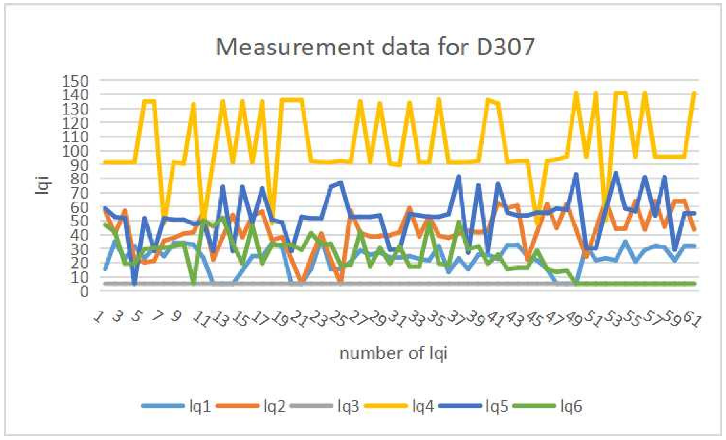
4.2. Signal Fluctuation Problem

Because of the low transmission power and the narrow channel bandwidth, the signal fluctuation problem can often happen at IEEE802.15.4, where the LQI of the received signal is fluctuated. This problem may appear when a person is moved around, a door is opened or closed, and another wireless signal at the 2.4 GHz is activated in the room, and will decrease the detection accuracy of FILS15.4.

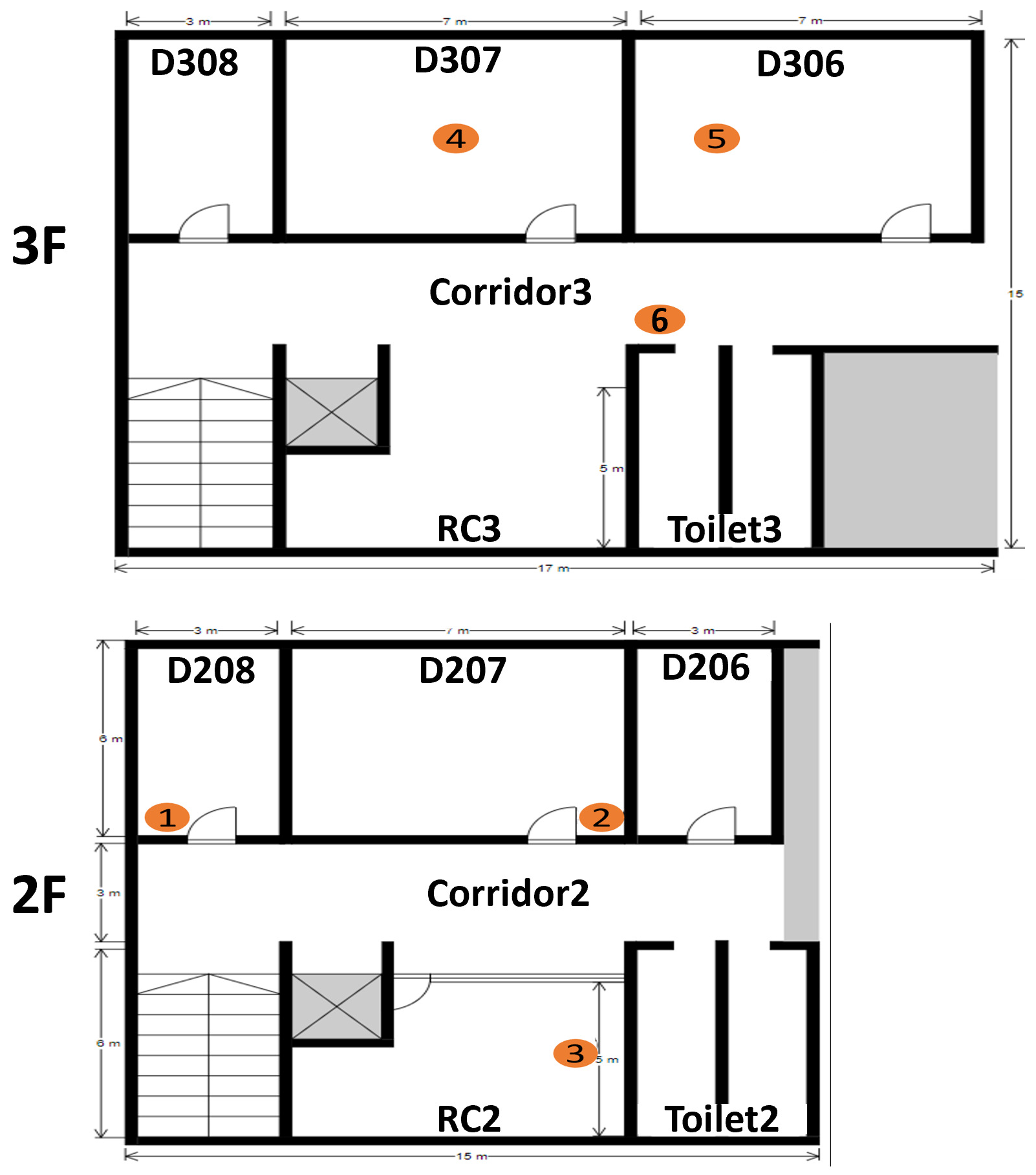
In our previous experiments, we fixed the transmitter in D307, and collected LQI data for 30 min at the six receivers located on the second and third floors of No. 2 Engineering Building at Okayama University as shown in Figure 1. Figure 2 suggests the signal fluctuation problem. Here, $LQI=5$ indicates that the receiver cannot receive any data from the transmitter where the connection loss happened.

To accomplish high detection accuracy by solving the signal fluctuation problem on IEEE802.15.4 devices, we limit the detection granularity of FILS15.4 to one room in the field. Furthermore, we make multiple fingerprints with distinct values for each room. As a result, the optimization of the number of fingerprints and their values for each room becomes an important issue in determining the detection accuracy of FILS15.4, which will be very difficult to achieve manually.

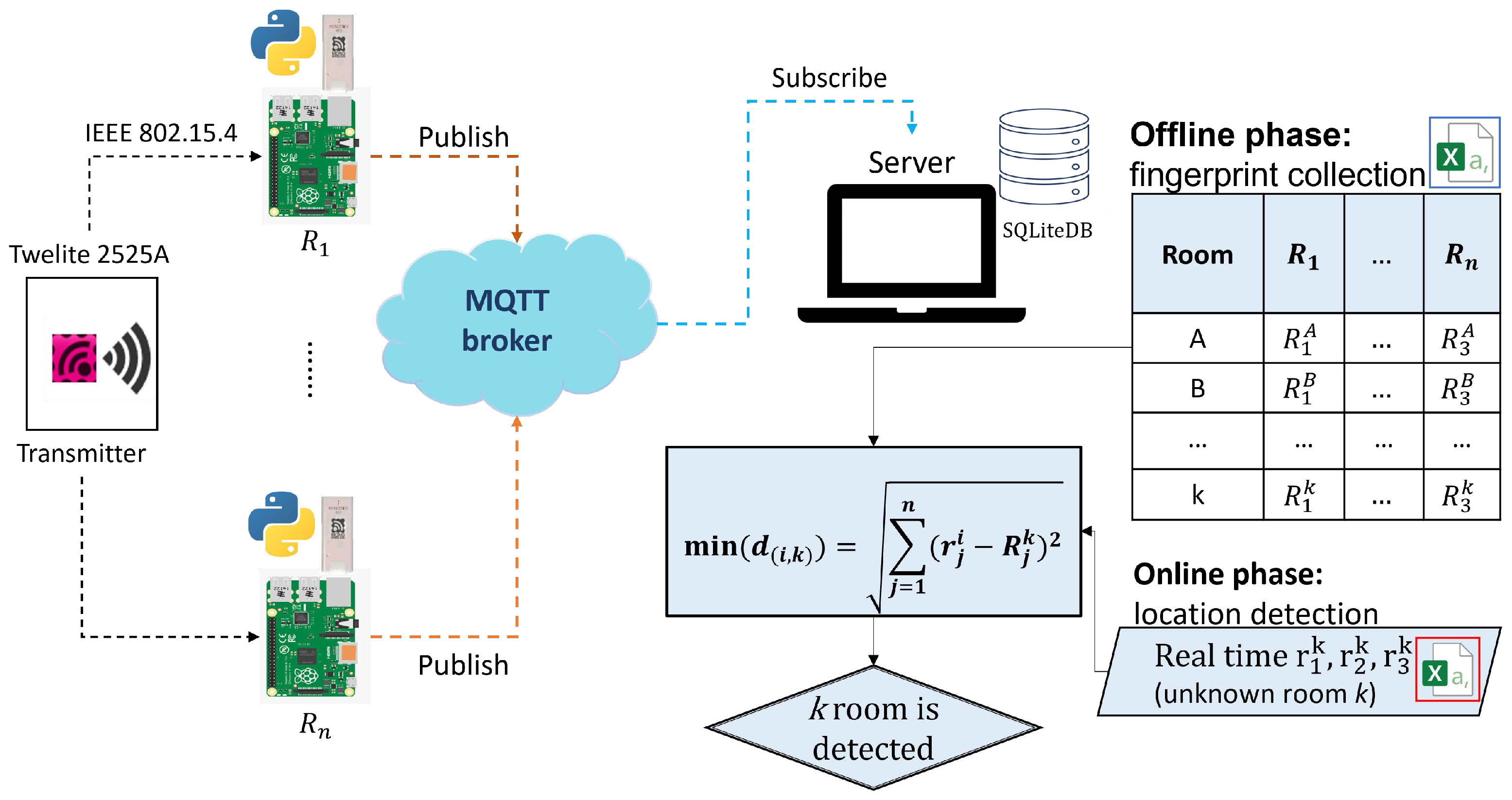
4.3. Implemented System

Figure 3 illustrates the overview of FILS15.4. During location detections, the user needs to always wear the transmitter device. The transmitter will send data with the 500 ms interval. The receivers allocated in the field will receive the data with $LQI$, and send them to the server through the USB-connected Raspberry Pi with the 30 s interval, utilizing the MQTT protocol. The server detects the user’s current room by comparing the received $LQI$ with every stored fingerprint.

FILS15.4 adopts Twelite 2525 in Mono Wireless [2] as the transmitter conforming the IEEE 802.15.4 standard. The wireless signal is at the 2.4 GHz band, which can be interfered with IEEE 802.11 Wi-Fi. During detections, the user may wear it at the wrist.

Furthermore, FILS15.4 adopts Mono Stick in the same company as the receiver. It is connected with Raspberry Pi through the USB interface. When a packet from a transmitter is received, the link quality indication (LQI) is also monitored. Raspberry Pi sends the received and LQI data to the server through the MQTT protocol [17].

In the calibration phase, the server stores the received data in the SQLite database, calculates the average LQI during every 30 s, and combines the values from all the receivers into one vector to generate the fingerprint for the room. It is stored with the relevant location label. In the detection phase, the server calculates the Euclidean distance between the average measured LQI and every fingerprint to detect the current room at every 30 s.

4.4. Localization Logic and Parameters

As the initial parameter values, one is used for the initial value of the number of fingerprints, and the average of all the measured LQI data at a receiver from a transmitter located in the target room is used for the initial value of the corresponding fingerprint value.

(1)

Properly locate the Raspberry Pi devices with the receivers in the target field.

(2)

Run the programs and create the connection to the MQTT broker.

(3)

Locate the transmitter at the specified location in the field. In our experiments, we selected several locations where we moved the transmitter from one place to another after measuring LQI for one minute by transmitting packets every 500 ms.

(4)

Receive and collect the packets from the transmitter at the Raspberry Pi device for 30 s.

(5)

Forward the collected data from the Raspberry Pi device to the server through the MQTT broker.

(6)

For each receiver, calculate the average LQI using the forwarded data from it after the last average LQI calculation.

(7)

Make the fingerprints at the server and store them in the SQLite database.

In the detection phase, the server detects the current room of the user by applying steps (1)–(6) in the procedure for the calibration phase periodically. Then, in step (7), after the vector of the average LQI values from all the receivers are obtained, the Euclidean distance is calculated against every pre-stored fingerprint by Equation (2), and the room whose fingerprint has the smallest distance is appointed as the detected room.

$$dis{F}_i^k=\sqrt{\sum _{j=1}^n{(r_j^i-R_j^k)}^2}$$

(2)

where

• $dis{F}_i^k$ represents the Euclidean distance between the i-th measured average LQI and the fingerprint for room k;
• $r_j^i$ does the i-th measured average LQI at receiver j; and
• $R_j^k$ does a fingerprint for room k at receiver j.

4.5. Parameter Optimization Algorithm Application

FILS15.4 has several parameters whose values should be optimized. The following procedure describes the calculation of the score $S\left(P\right)$:

(1)

Calculate the Euclidean distance $dis{F}_i^k$ between the i-th average measured LQI and the k-th current fingerprint.

(2)

Find $dis{F}^{OK}$ that represents the minimum Euclidean distance against a fingerprint representing the correct room.

(3)

Find $dis{F}^{NG}$ that represents the minimum Euclidean distance against a fingerprint representing the incorrect room.

(4)

Calculate $S\left(P\right)$ by:

$$S\left(P\right)=A\sum _{i=1}^{N}true(dis{F}^{OK}-dis{F}^{NG})+B\sum _{i=1}^N\frac{dis{F}^{NG}}{dis{F}^{OK}}+C\sum _{k=1}^M\underset{b\ne c}{min}\mid F_b^k-F_c^k\mid$$

(3)

where A and B represent constant coefficients ($A=10$, $B=1$ and $C=1$ in this paper), N is the number of the average measured LQI for the optimization, the function $true\left(x\right)$ returns 1 if $x>0$ and 0 otherwise. The C-term represents the sum of the minimum Euclidean distance between two different fingerprints for the same room. It intends to generate different fingerprint values for the same room.

Moreover, as the important parameters in paraOpt, $t_i=10$ for the tabu period, $\Delta p_i=5$ for the detection interval, and $\Delta p_i=1$ for the fingerprint are adopted.

4.6. Evaluations

The field layout in Figure 1 is used in experiments. Among the parameters in FILS15.4, the detection interval and the fingerprint values can most influence the detection accuracy. Thus, their optimizations are discussed.

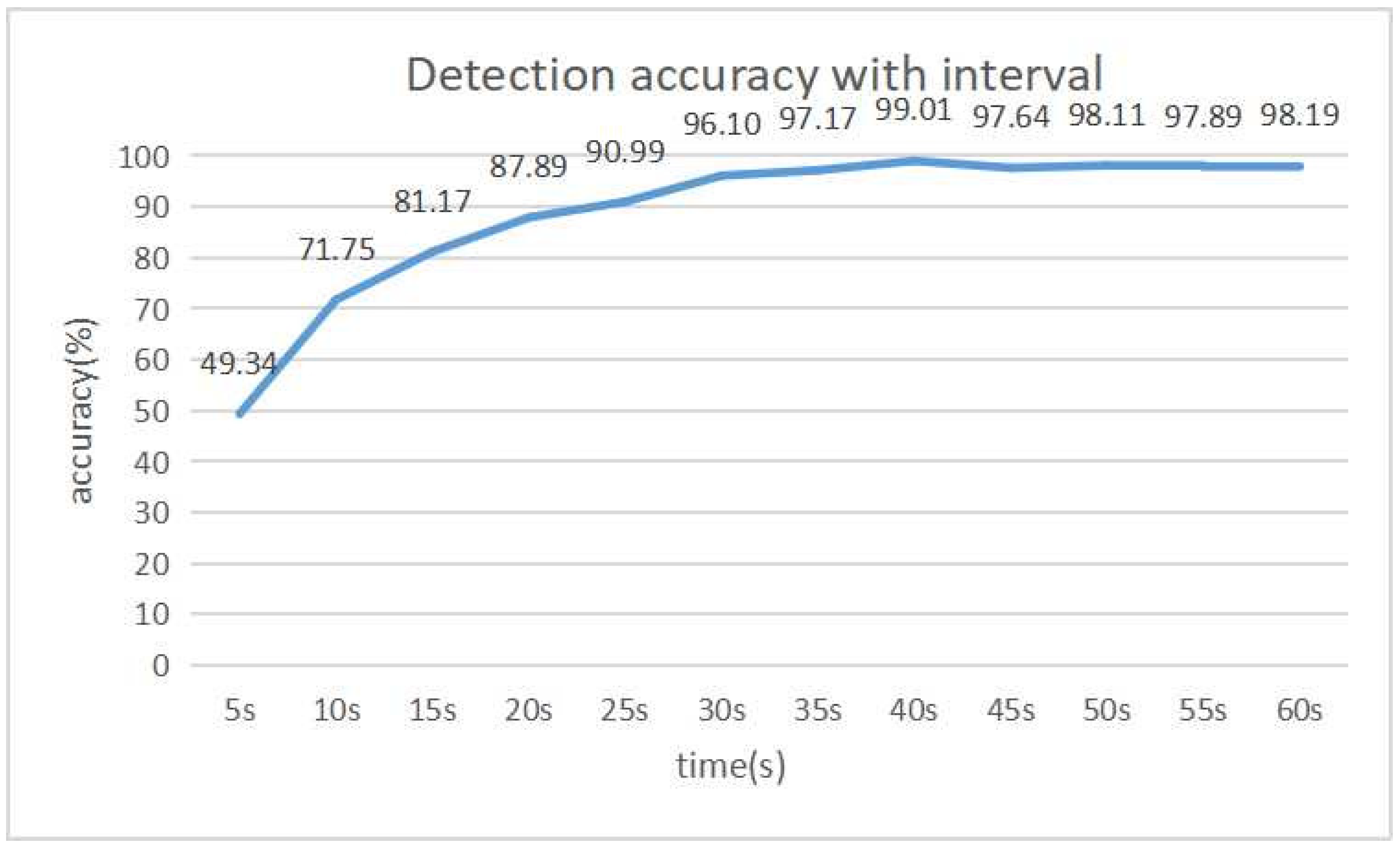
4.6.1. Optimization of Detection Interval

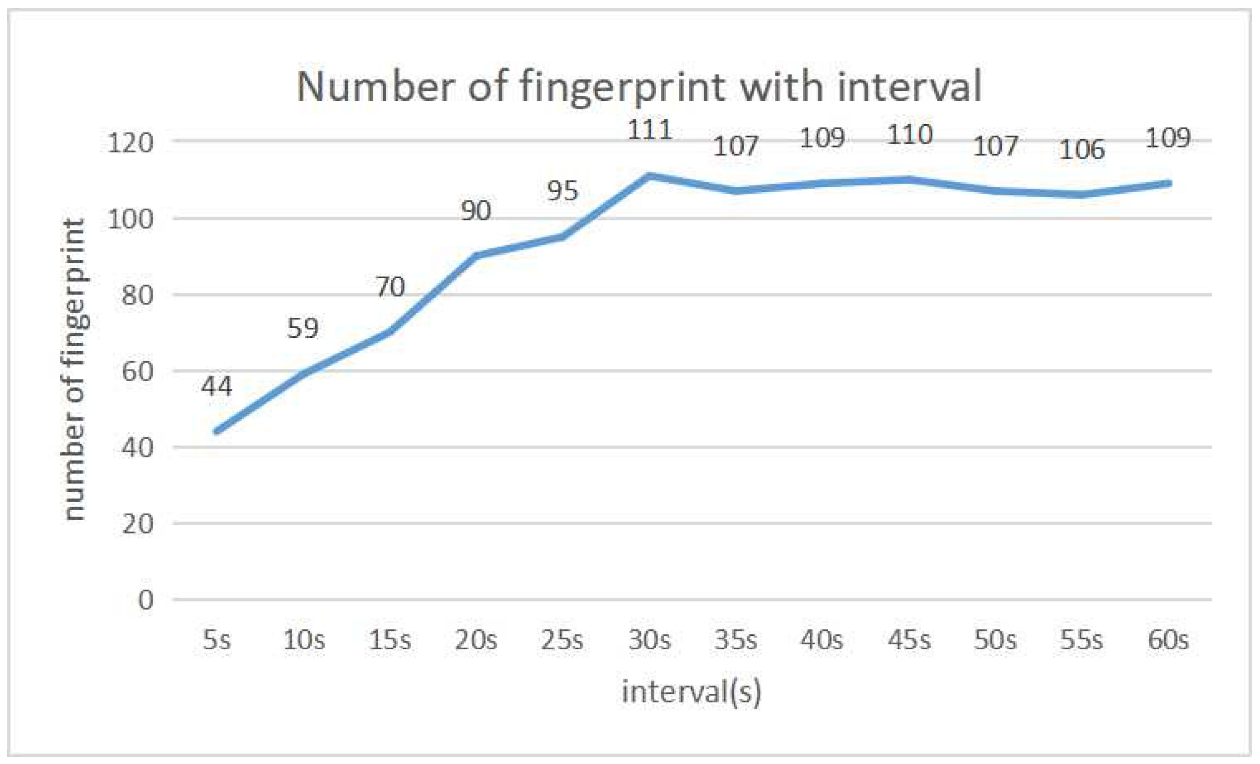
First, the detection interval is optimized. Figure 4 and Figure 5 show the detection accuracy and the number of fingerprints for each interval respectively. From 0 s to 30 s, both the detection and the number of fingerprints gradually increase. Then, both are saturated. The best detection accuracy is obtained when the interval is 40 s, where the total number of fingerprints is 109.

4.6.2. Optimization of Fingerprints

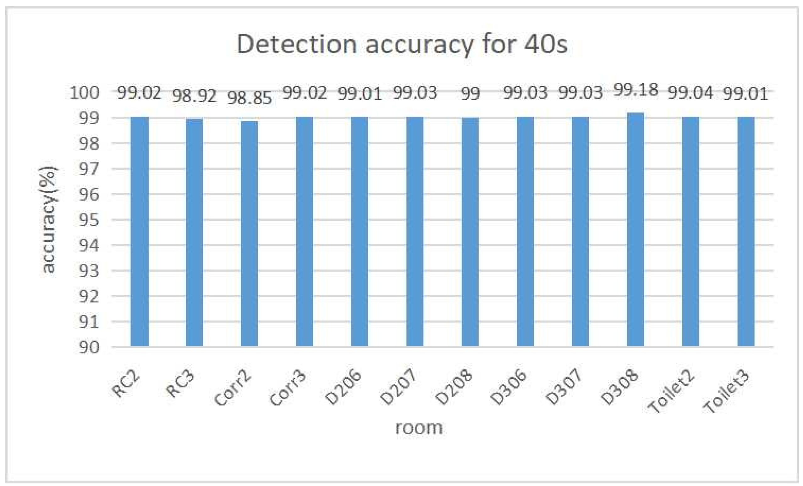
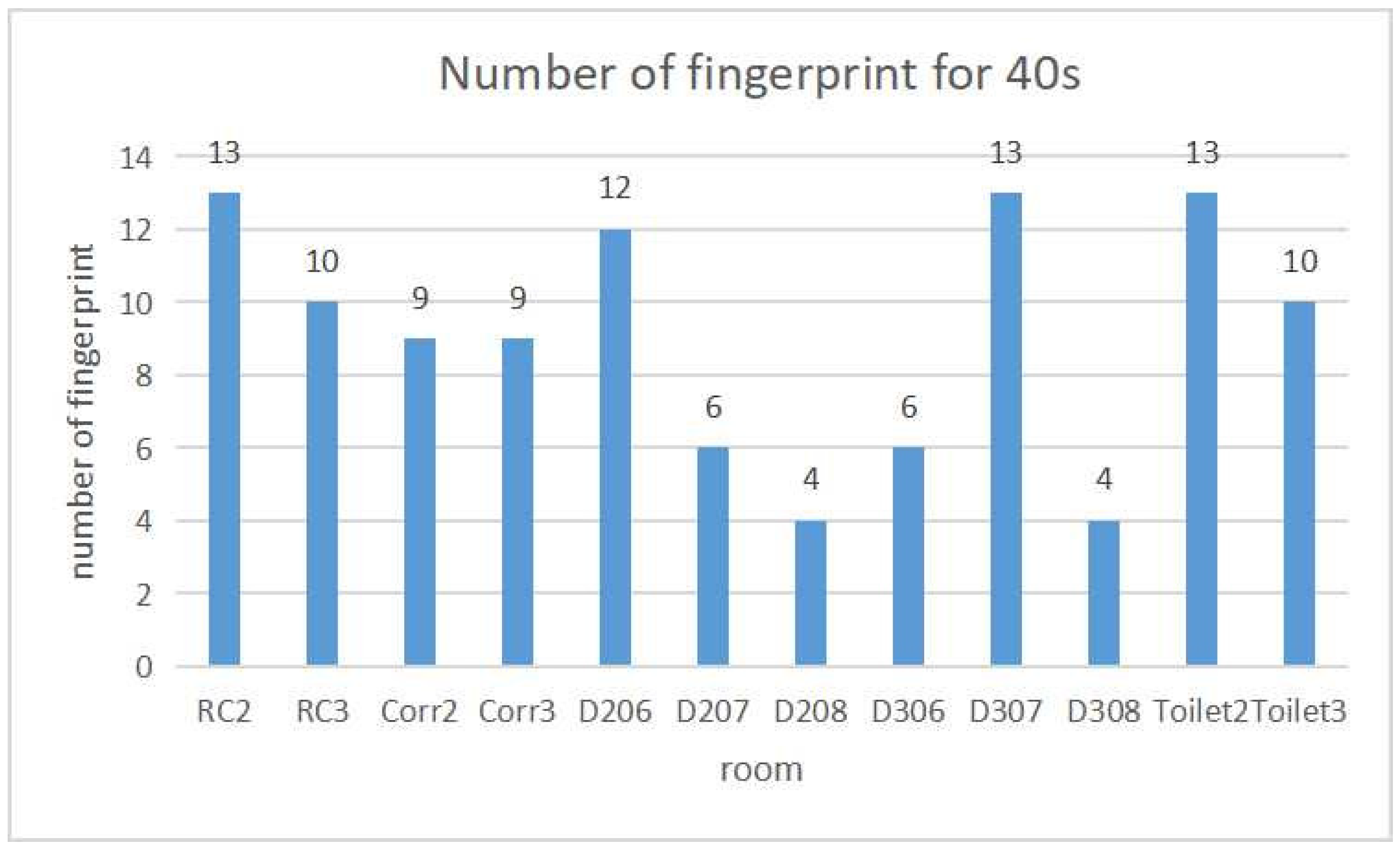
Figure 6 and Figure 7 show the detection accuracy and the number of fingerprints for each room respectively when the detection interval is 40 s. The largest number of fingerprints is 13 for RC2, D307 and Toilet2. The least number of fingerprints is four for D208 and D308.

4.6.3. Discussions

Since the measured LQI is frequently fluctuating, the moving average should be used instead of the instantaneous value to reduce misdetections. Then, the time period of the average, or the detection interval should be optimized to maximize the detection accuracy.

Then, the results in Figure 4 and Figure 5 indicate that the detection accuracy is improved until the interval becomes 40 s. After that, the accuracy is saturated, where the number of fingerprints is also saturated. Thus, 40 s is selected as the best detection interval.

It is noted that the results were obtained when all the transmitters were stationary or not moving. The detection interval should be optimized when transmitters are sometimes moving in the field. However, variations of transmitter/user movements are much more diverse, including source/destination locations, moving speeds, and paces. A lot of experiments will be necessary to find the optimal interval. Thus, it will be in future works.

With the fixed detection interval of 40 s, Figure 6 shows a sufficiently high detection accuracy of higher than $98\%$ for any room. Figure 7 shows the number of fingerprints generated by the proposal. For D208 and D308, only four fingerprints are necessary and are smaller than the other rooms. The reason is that both rooms are located at the end of each floor in the two-floor field and are isolated from the other rooms. It will cause less confusion with other rooms. On the other hand, the other rooms are surrounded by several rooms and need many fingerprints to reduce confusion among them.

4.7. Performance Comparison with GA

Here, for FILS15.4, we compare the performance of the proposal with GA that is implemented by modifying the source code in [18]. This GA code has been applied to the input data with multiple features such as FILS15.4.

4.7.1. GA Implementation

In the GA implementation, the number of chromosomes is set to 100, and the mutation rate is 0.1. The initial values of values and the room label for fingerprint are randomly generated between 5 and 151. The roulette selection algorithm is adopted. For a new chromosome generation from randomly selected two fingerprints, randomly selected one fingerprint is swapped between them. For a new room label, the room label of the fingerprint that has the smallest Euclidean distance among the fingerprints that caused misdetections to this room is changed to the label if the detection accuracy of one room is lower than $60\%$.

4.7.2. Comparison Results

Table 2. PC specifications.

Hardware	Model	Size
CPU	Intel core i5-10300H@2.50 GHz	Four cores
memory	SK Hynix DDR4 3200 MHz	16 GB
disk	Samsung MZVLB512HBJQ-000L2	512 GB

shows the PC specification to run it with the 30 s detection interval.

Table 3. Comparison between GA and ParaOpt.

Iterations	GA	paraOpt
100	62.5%	68.9%
1000	76.5%	89.8%
10,000	92.3%	95.3%

and

Table 4. CPU time.

Iterations	GA	paraOpt
100	11.96 s	11.21 s
1000	117.43 s	107.21 s
10,000	1162.07 s	1030.53 s

compare the average detection accuracy and the CPU time between GA and paraOpt when the same number of iterations is elapsed. It clearly shows the superiority of the proposal.

5. Application to Face Contour Approximation Model

In this section, we present the application of paraOpt to the human face contour approximation model.

5.1. Background

Face drawing has been a longstanding and distinct art. It typically uses a sparse set of continuous graphical elements such as lines to capture the distinctive appearance of a human. It will be done in the presence of a person or his/her face image, and rely on the holistic approach of observation, analysis, and experience [19].

The traditional technology to draw a human face contour may include four steps [20]. The first step is to draw a circle and a cross to represent the top portion of the head. The second step is to draw a square within the circle to represent the edges of the face. The third step is to draw the chin from each side of the square. The last step is to locate the hair and eyes by using lines.

For beginners, traditional technology can be hard to learn by themselves. Therefore, an application system should be developed to assist them to learn the drawing of the face contour. A lot of technologies can help draw the face contour, including AI technology [21,22].

5.2. Proposed Model and Parameters

In this paper, we present the use of OpenPose to assist in drawing the human face contour by beginners. OpenPose is the popular open software that can jointly detect the coordinates of the keypoints in the human body, hands, face, and foot from a single image [23]. A keypoint represents a feature point in them such as a joint, a fingertip, and a nostril. Since OpenPose will extract the contour of the chin, it can help extract the face contour. However, OpenPose cannot extract the contour of the upper part of the face including the forehead due to the hair.

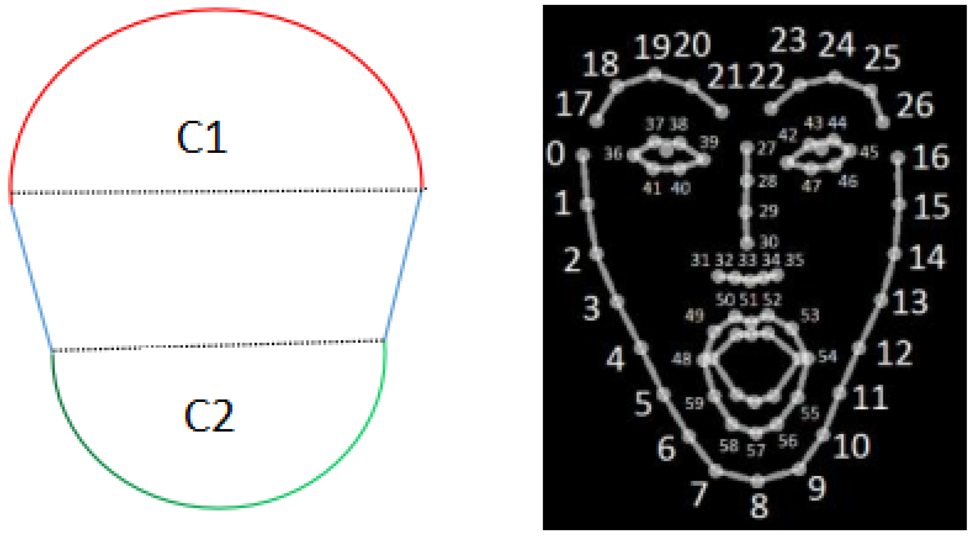
For solving this limitation, we propose a simple face contour approximation model that consists of two half circles and line segments. The upper half circle will draw the forehead and the lower half circle will draw the chin. The two line segments that connect the ends of the two half circles will draw the edges of the face contour. Then, the parameters of this model including the center coordinates and the radii of the half circles should be properly selected so that the resulting model is well matched with the keypoints by OpenPose. paraOpt is applied to the optimization of the parameters. Figure 8 illustrates the face contour approximation model and the related keypoints by OpenPose, which is obtained from [24].

5.3. Model Generation Procedure

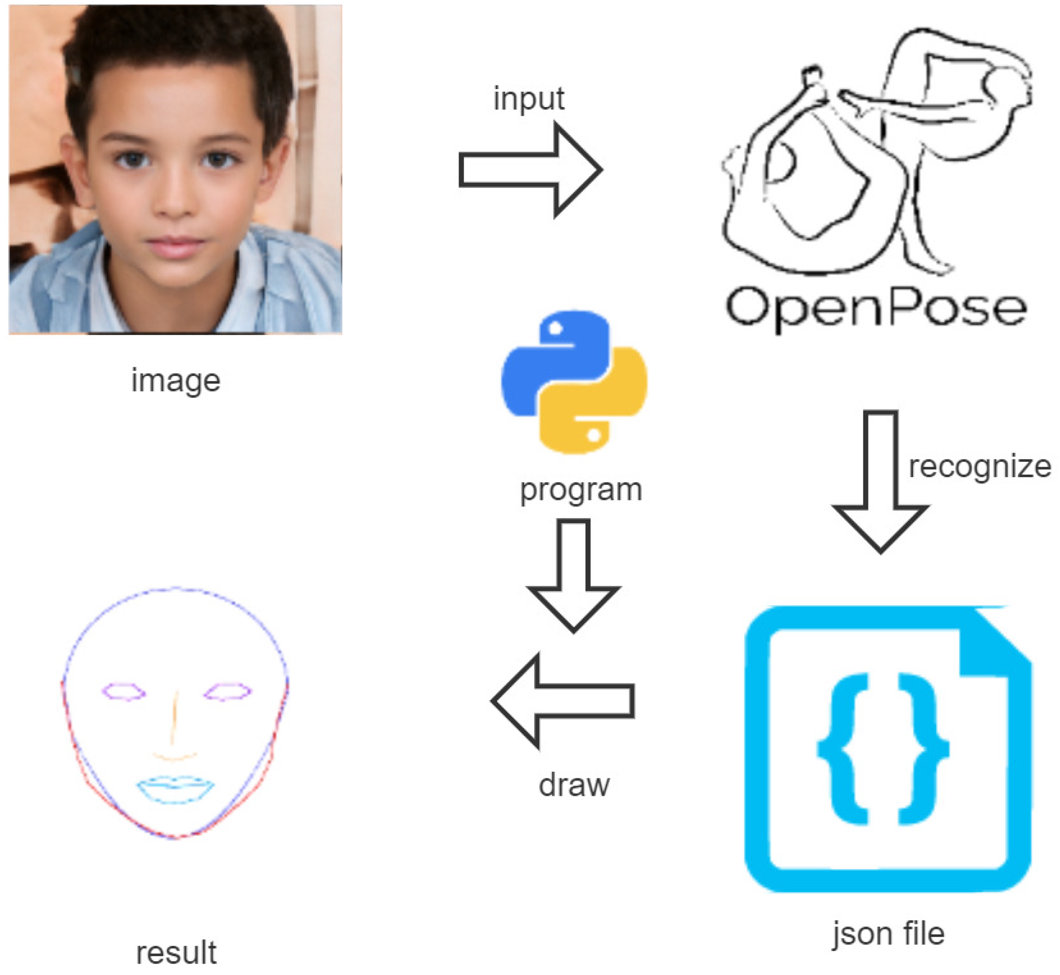
Figure 9 shows the procedure of generating the face contour approximation model. It is noted that the image in this figure was generated by using the online deep learning model [25]. First, the user prepares the face image to be drawn. Second, by applying the image to OpenPose, the keypoints of the face are extracted from the image and saved into the Json file. Finally, our Python program for paraOpt reads the keypoints and optimizes the parameters of the model.

5.4. Initial Parameter Values

The initial values of the parameters are obtained from the related keypoint coordinates. For the upper half circle C1, keypoint 27 of Openpose is used for the center, and the Euclidean distance between two keypoints 27 and 16 is used for the radius. For the lower half circle C2, keypoint 33 is used for the center, and the distance between keypoints 33 and 8 is used for the radius.

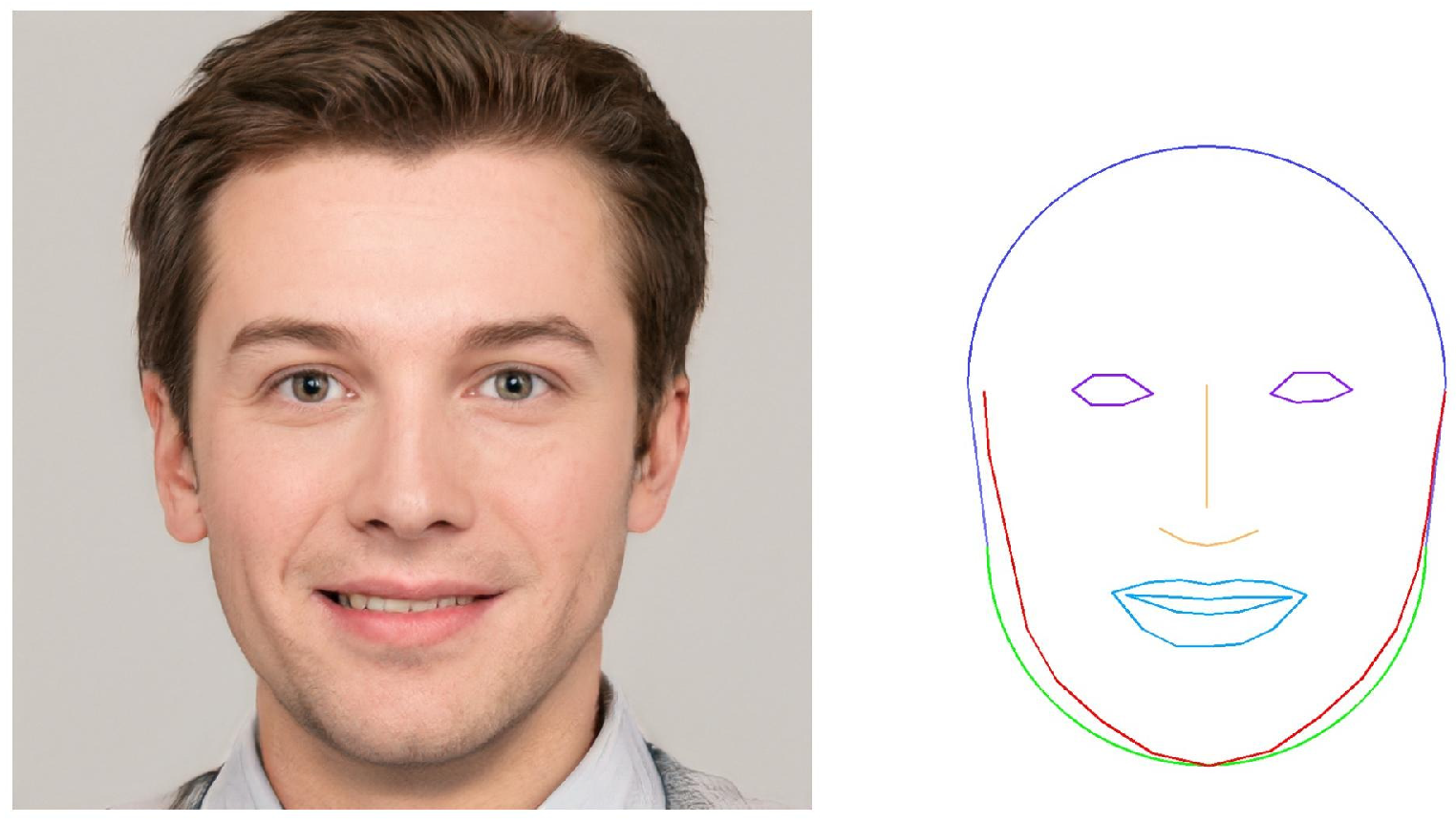
5.5. Example Initial Model

Figure 10 shows the example image and the face contour model using the initial parameter values. This image was also generated by using the online deep learning model [25]. The red line represents the contour that is given by tracing the keypoints by OpenPose, and the green line represents the model. Some differences can be recognized between them. Thus, the parameters of the model should be optimized.

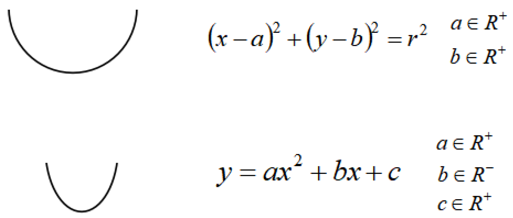
5.6. Alternative Model

It has been observed that the chins of some persons are not round but rather sharp. For such faces, an alternative model is proposed. Here, instead of the lower half circle, a quadratic curve shown in Figure 11 is used, which was originally drawn in this paper. The initial values of the three coefficients, a, b, and c, are calculated by solving the equations that will be introduced by assuming that this quadratic curve will cover the three keypoints 2, 8, and 14.

5.7. Score Function

To optimize the parameters of the human face contour approximation, the score function $S\left(P\right)$ is calculated by the following procedure:

(1)

Calculate the Euclidean distance between each of the 17 keypoints (0∼16) and keypoint 33 in the OpenPose result in Figure 8 respectively.

(2)

Find the corresponding coordinate on the function of the proposed model to each of the 17 keypoints by calculating the y coordinate on the function that has the same x coordinate.

(3)

Calculate the Euclidean distance between each corresponding point to the 17 keypoints and the keypoint 33 respectively.

(4)

Calculate the score function $S\left(P\right)$ by:

$$S\left(P\right)=\sum _{i=0}^{16}|E_i^k-E_i^s|$$

(4)

where $E_i^k$ represents the Euclidean distance between keypoint i for i = 0∼16, and keypoint 33, and $E_i^s$ denotes the Euclidean distance between the corresponding coordinate on the model function and keypoint 33.

In the parameter optimization algorithm, tabu $t_i$ = 10, and $\Delta p_i$ = 1 are used.

5.8. Evaluations

Here, we evaluate the proposal for the human face contour approximation model.

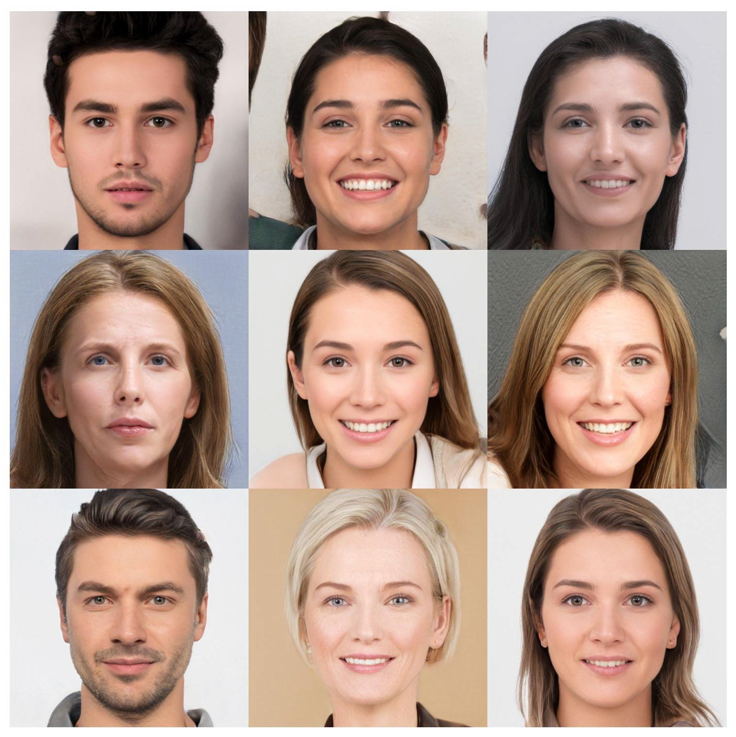
5.8.1. Face Images

For evaluations, 200 face images with $1024\times 1024$ pixels are collected from an online site. They are artificially generated using the deep learning model, including both genders, and various ages and races. Figure 12 shows some of them that were generated by the online deep learning model [25].

5.8.2. Optimization Results

Table 5. Parameter optimization results.

Model	#	Before Optimization	After Optimization
half circle	21 (10.5%)	473.51	448.80
quadratic curve	179 (89.5%)	274.31	263.05

shows the number of images that selects each model, and the average score results before and after applying paraOpt for all the images. The results suggest that most chin shapes can be approximated by a quadratic curve, where the score is smaller than that for the half circle.

Ideally, the score should be zero where all the 17 keypoints are on the model function. However, it is not realistic, because the adopted model functions may not well represent the face contour, and OpenPose usually make some errors on keypoints. It is necessary to find and define proper model functions that will reduce the scores depending on human faces. It will be in future works.

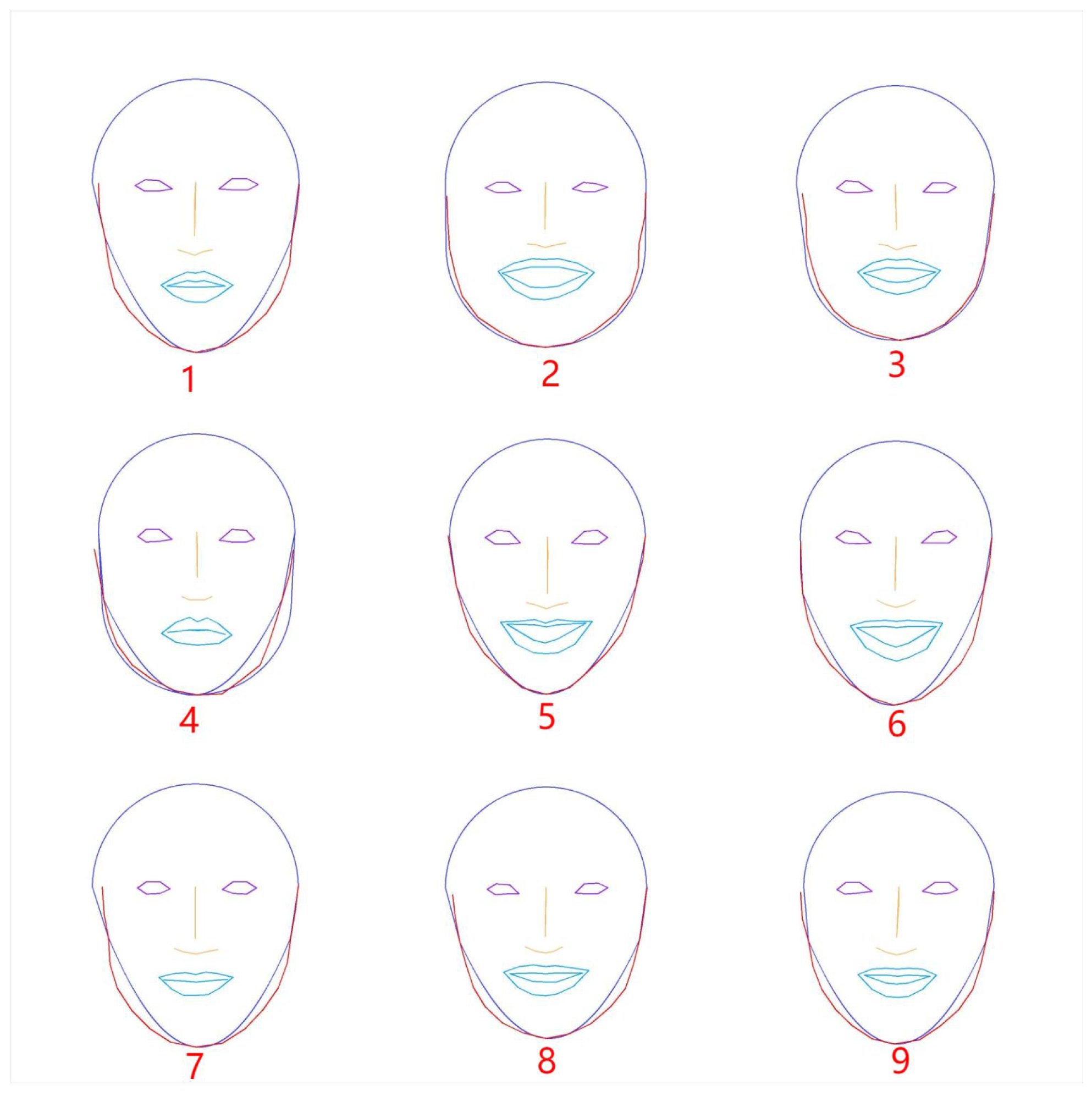
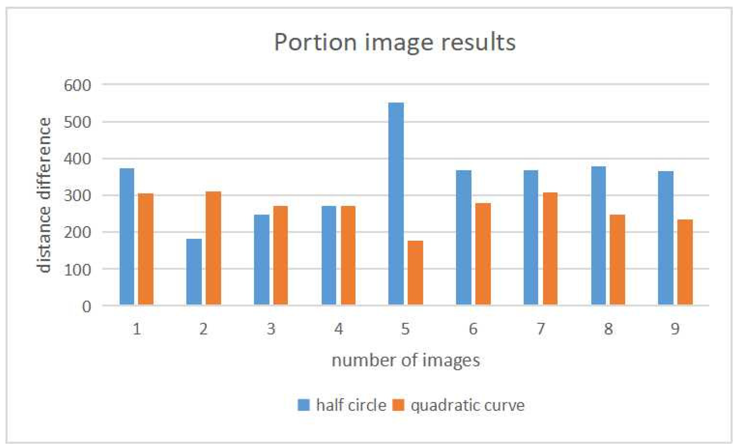
Figure 13 depicts the results of the face contour approximation models and the keypoints in faces by OpenPose for the nine face images in Figure 12. Figure 14 compares the score results between the two models. The half circle model is better for only three images of 2, 3, and 4. The score difference between the scores is larger for the images where the quadratic curve model is better.

5.9. Performance Comparison with GA for Face Model

Here, for Face Contour Approximation Model, we compare the performance of the proposal with GA that is implemented by modifying the source code in [18].

5.9.1. GA Implementation

For Face Contour Approximation Model, the number of chromosomes is set to 10, and the mutation rate is 0.1. The initial values of the coefficients for half circle and quadratic curve is randomly generated between 1 and 100. The roulette selection is adopted. For the new chromosome generation, the randomly selected one coefficient is swapped between the randomly selected two chromosomes.

5.9.2. Comparison Results

Table 2 shows the PC specification.

Table 6. Average Euclidean distance for Face Contour Approximation Model.

Iterations	GA	paraOpt
100	323.65	315.65
1000	303.15	303.15
10,000	295.76	295.76

and

Table 7. CPU time for Face Contour Approximation Model.

Iterations	GA	paraOpt
100	20.56 s	13.99 s
1000	17.96 s	17.80 s
10,000	30.53 s	22.93 s

compare the average Euclidean distance and the CPU time between GA and paraOpt when the same number of iterations is elapsed. Since the number of data is not large, the accuracy is similar between GA and paraOpt where the CPU time is shorter for paraOpt.

6. Application to CFD Simulation

In this section, we present the application of paraOpt to the CFD simulation using OpenForm.

6.1. Overview

Nowadays, air conditioners (ACs) are equipped in many rooms in houses, schools, factories, and offices to offer comfortable environments for humans and machines. On the other hand, global warming has been escalated due to overconsumption of fossil fuels. Therefore, the proper use of ACs has become more important around the world.

Then, the estimation or prediction of the distributions of the temperature or humidity in a room using a simulation model will be useful to properly control ACs. By estimating the room environment changes under various actions, it will be possible to decide when ACs be turned on or off. Even, the timing to open or close windows in the room can be selected.

ACs rely on a limited number of sensors for measuring the temperature and humidity in the room. Therefore, to obtain the distribution of the temperature or humidity in a room, additional sensors should be used together by externally allocated in the room, which is not practical. Moreover, the sensors cannot predict future changes of them.

To estimate or predict the distributions in a room together with sensors, we are investigating the CFD simulation using OpenFOAM software [26]. Then, the optimization of the parameters in OpenFOAM is critical in order to fit well the simulation results with the corresponding measured ones.

6.2. Model Room for Experiments

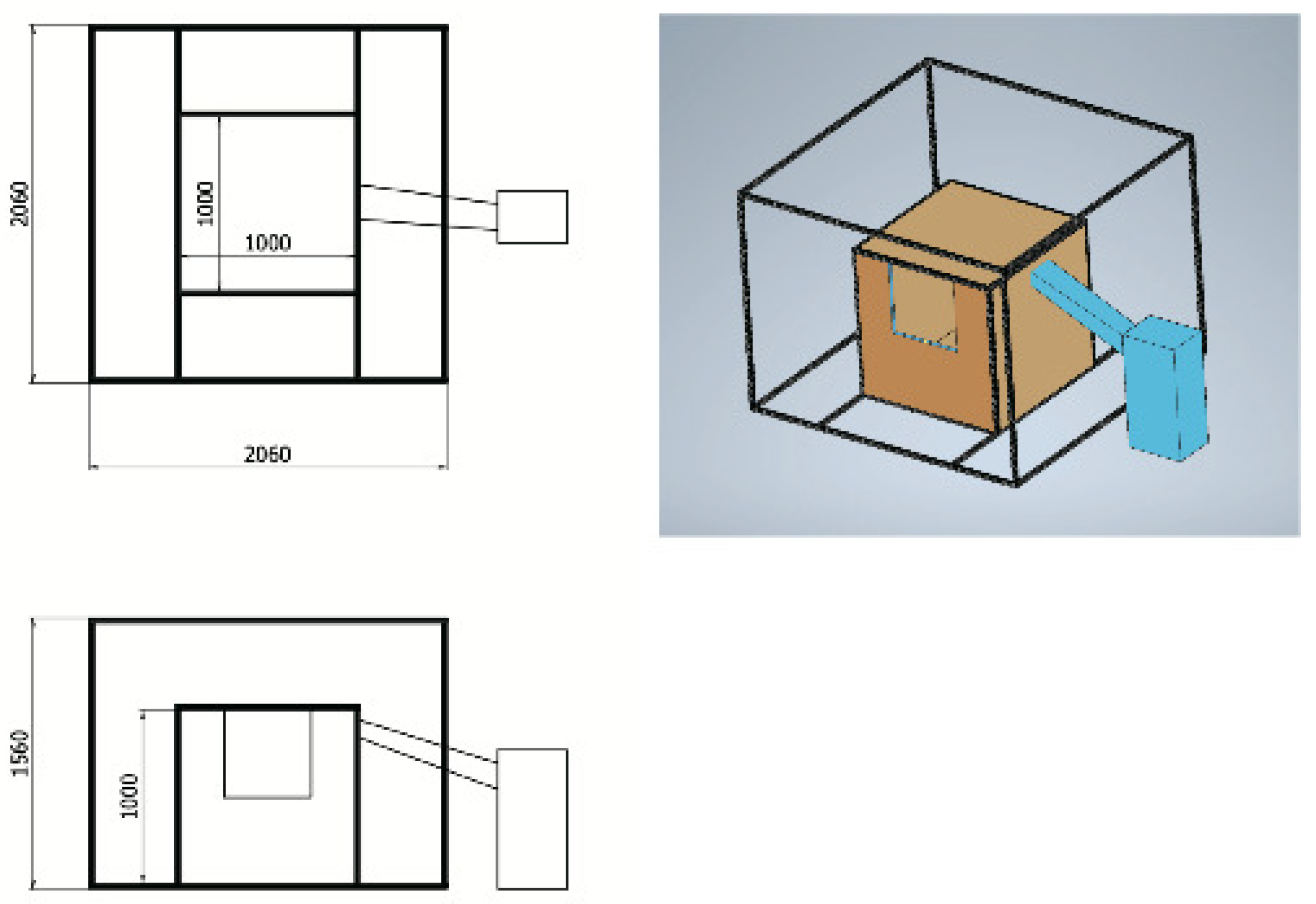
In a real room, it is very difficult or impossible to freely change the temperature or humidity to be the required one in the experiment under various weathers or seasons. To solve this problem, a small-sized model room for experiments in Figure 15 is assembled for this study. The size of this model room is 1 m × 1 m × 1 m, and is covered by the outer box whose size is 2 m × 2 m × 1.5 m. The walls of this box are insulated with the 30 mm thick insulation. In the model room, temperature-controlled air using an air conditioning unit can be supplied. Furthermore, at the bottom of the model room, the heaters are mounted to raise the temperature. To measure the temperature distribution of the room, 27 temperature sensors are installed at equal intervals in the room.

6.3. CFD Simulation Model and Parameters

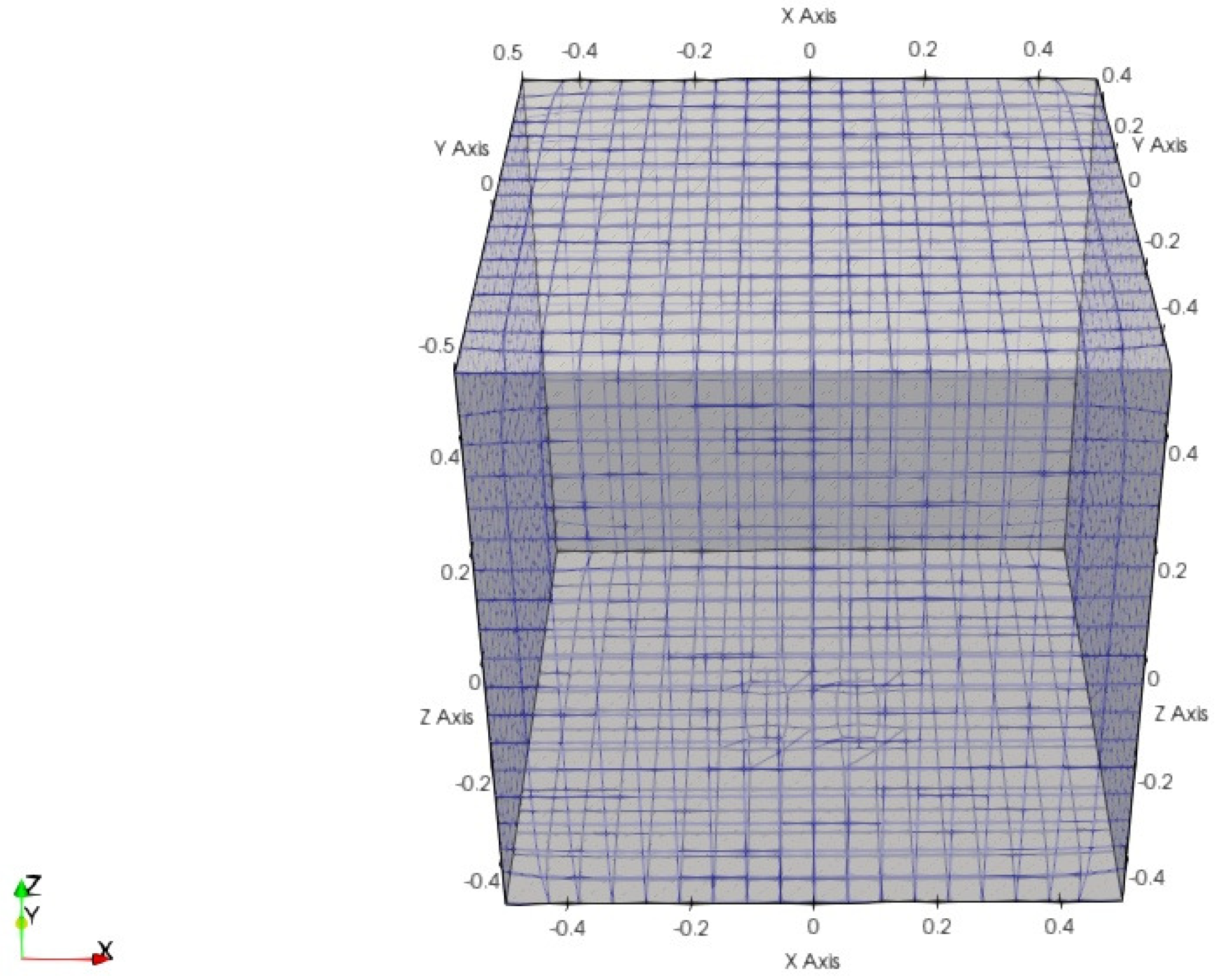
To estimate the temperature distribution of the model room, the CAD model for OpenFOAM in Figure 16 is made to represent the room. The dimension of the CAD model is the same as the real one.

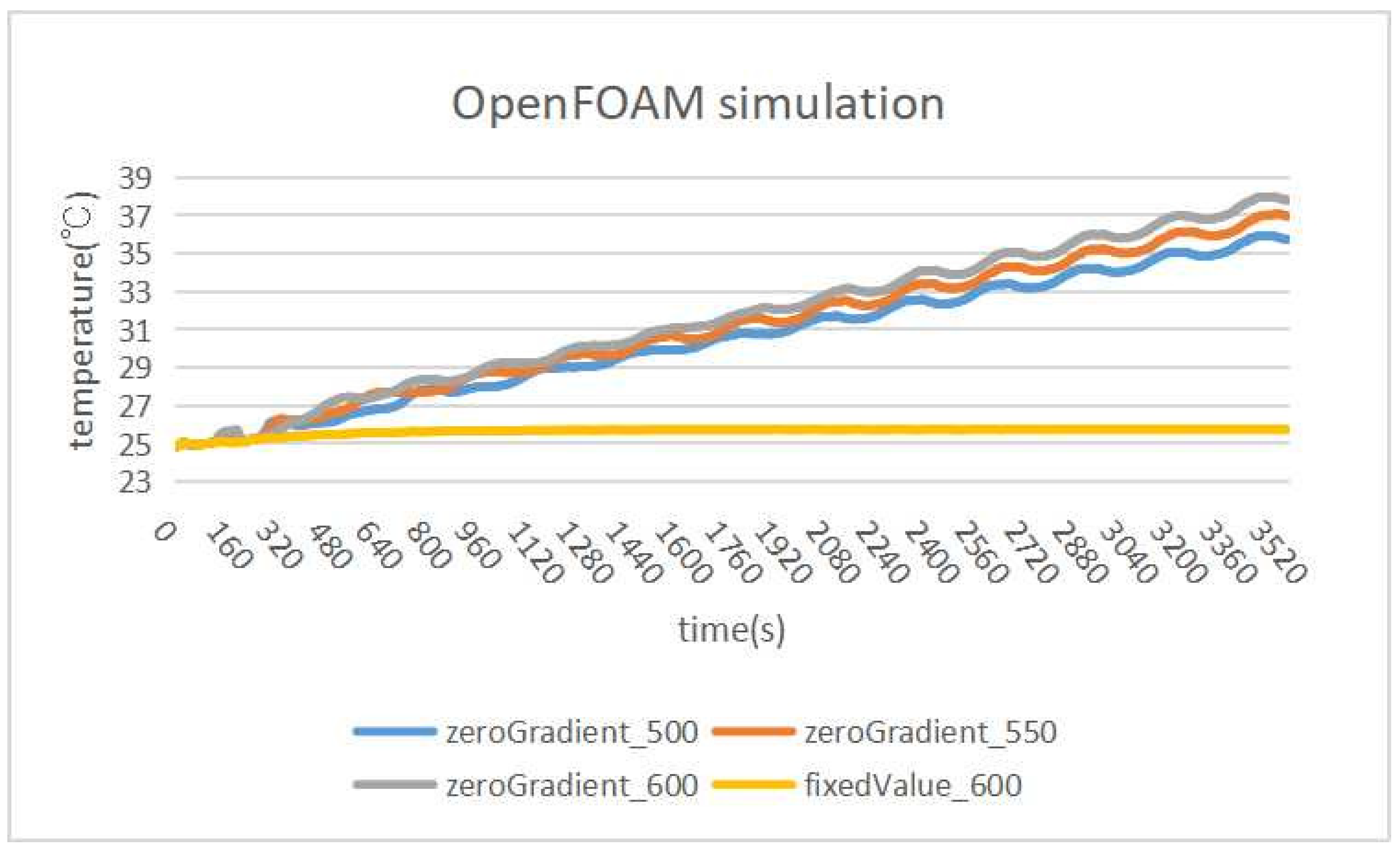
Before starting the CFD simulation using OpenFOAM, the boundary conditions for the walls and the heater need to be set properly, since they strongly influence the simulation result.

Table 8. Boundary conditions.

Wall	zeroGradient	zeroGradient	zeroGradient	fixedValue
heater	500	550	600	600

shows some examples of them. The zeroGradient represents the adiabatic condition and fixedValue represents the wall having a fixed temperature. The boundary condition of the heater is given by heat flux that will be presented later. The origin coordinate (0, 0, 0) in the CAD model is selected as the monitoring point because the sensor is mounted there. Figure 17 shows some simulation results.

6.4. Heat Flux Simulation

OpenFOAM cannot directly set the temperature condition for the heater in the simulation as can be done in reality. Instead, we use the following heat flux equation for the heating condition:

$$q=\lambda \frac{\Delta T}{\Delta x}$$

(5)

where

• q represents the heat flux, where the unit is W/m${}^2$.
• $\lambda$ represents the thermal conductivity through a specified material, which is expressed as the amount of heat that flows per unit of time through a unit area with a temperature gradient of one degree per unit distance.
• $\Delta T$ represents the difference between the outside and inside temperatures of the wall, where the unit is Kelvin(K).
• $\Delta x$ represents the thickness of the wall, where the unit is meter (m).

6.5. Score Function

The boundary conditions of the walls have a large influence on the temperature changes in the room. To accurately predict the temperature changes, the values of the boundary condition parameters in OpenFOAM should be optimized. The score function $S\left(P\right)$ is calculated from the given simulation heat flux values P and the measured temperatures by the following procedure:

(1)

Record the simulation temperature every five seconds for one hour.

(2)

Calculate the absolute value of difference simulation temperature between measurement actual temperature.

(3)

Calculate $S\left(P\right)$ by:

$$S\left(P\right)=\sum _{i=0}^N|T_s^i-T_m^i|$$

(6)

where $T_s^i$ does the i-th simulated temperature at every five seconds, $T_m^i$ does the i-th measured temperature saved at every five seconds, and N does the total number of temperatures. In the parameter optimization algorithm, tabu $t_i$ = 10 and $\Delta p_i$ = 10 are used.

6.6. Evaluations

Here, we evaluate the proposal for the CFD simulation through experiments using the model room.

6.6.1. Experiment Setup

In experiments, the initial boundary conditions in

Table 9. Parameters values before proposal.

Number	Mesh	Heater	Boundary Condition of Wall
pattern1	10,000	heat flux 500	zeroGradient
pattern2	10,000	heat flux 500	fixedValue

are used. zeroGradient represents the adiabatic condition of the wall. fixedValue represents that the outside of the wall has a fixed temperature. The initial temperature of the room including the inside and outside of the wall is $24.85{}^{\circ }$C. As the critical boundary condition parameter, the value of heat flux is optimized by paraOpt, where the values in Table 9 are used as the initial values.

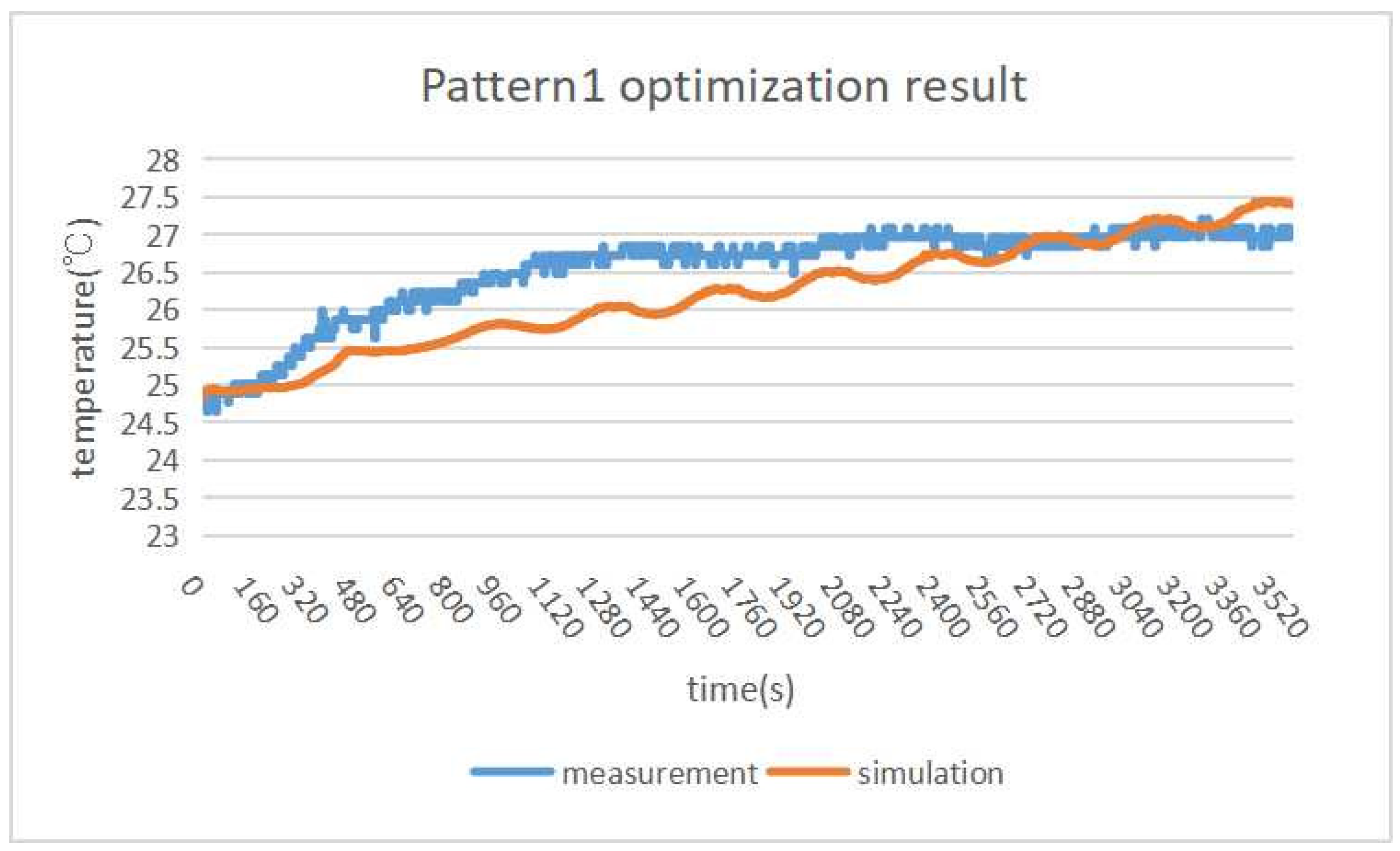
6.6.2. Optimization Results

Figure 18 and Figure 19 show the CFD simulation results after optimizing the parameters using paraOpt with pattern1 and pattern2, respectively. When the two results are compared, pattern2 is better.

In pattern1, paraOpt finds 100 W/m${}^2$ for the optimal heat flux value. Figure 18 compares the measurement and simulation temperatures. Although the heat flux is relatively small, the room temperature increases rapidly, and continues to increase. Here, due to the adiabatic condition, no heat is dissipated to the outside of the room. However, the measurement temperature is saturated and the heat is dissipated outside the room, which suggests that the walls are not adiabatic.

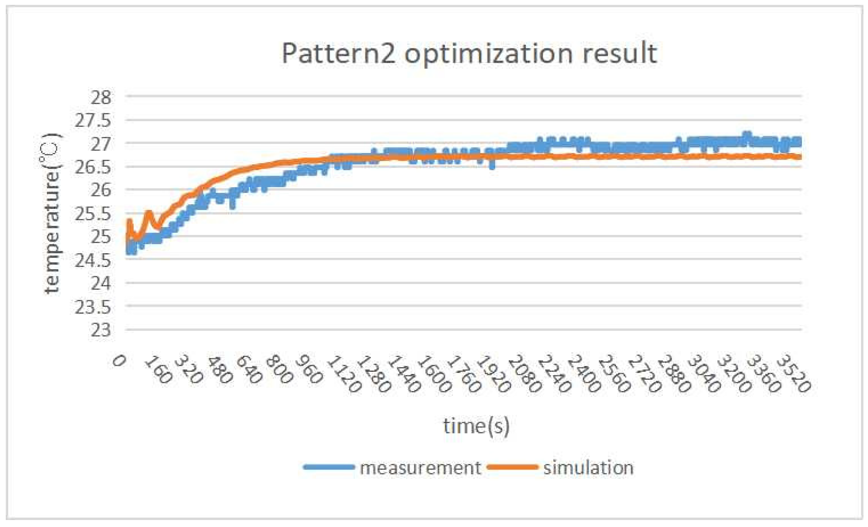
In pattern2, paraOpt finds 1390 W/m${}^2$ for the optimal heat flux value. Figure 19 shows that the measurement and simulation temperatures are similar, where the temperature difference is only $0.22{}^{\circ }$C. paraOpt can find the proper parameter value with the proper assumption of the simulation model.

6.7. Performance Comparison with GA for CFD Model

For CFD Model, we compare the performance of the proposal with GA that is implemented by modifying the source code in [18].

6.7.1. GA Implementation

For CFD Model, the number of chromosomes is set 10, and the mutation rate is 0.1. The initial values of values for heat flux are randomly generated between 100 and 3000. The roulette selection algorithm is adopted. For a new chromosome generation, one randomly selected heat flux is swapped.

6.7.2. Comparison Results

Table 2 shows the PC specification.

Table 10. Temperature for pattern1 of CFD model.

Iterations	GA	paraOpt
100	$1.5{}^{\circ }$C	$1.3{}^{\circ }$C
1000	$0.9{}^{\circ }$C	$0.9{}^{\circ }$C
10,000	$0.9{}^{\circ }$C	$0.9{}^{\circ }$C

,

Table 11. Temperature for pattern2 of CFD model.

Iterations	GA	paraOpt
100	$0.8{}^{\circ }$C	$0.6{}^{\circ }$C
1000	$0.22{}^{\circ }$C	$0.22{}^{\circ }$C
10,000	$0.22{}^{\circ }$C	$0.22{}^{\circ }$C

,

Table 12. CPU time for pattern1 of CFD model.

Iterations	GA	paraOpt
100	63.75 s	55.32 s
1000	527.06 s	450.52 s
10,000	6372.54 s	6145.73 s

and

Table 13. CPU time for pattern2 of CFD model.

Iterations	GA	paraOpt
100	55.45 s	53.01 s
1000	436.87 s	382.14 s
10,000	6238.82 s	6075.87 s

compare the average temperature and the CPU time between GA and paraOpt when the same number of iterations is elapsed. The accuracy is similar between GA and paraOpt where the CPU time is shorter for paraOpt.

7. Discussions on Three Applications

In this section, we summarize and discuss the results in the three applications of the proposal in this paper.

7.1. Performances in Three Applications

We discuss the performances of paraOpt in the three applications.

First, we examine the effectiveness of the proposed algorithm by comparing the accuracies in the three applications before and after applying it.

Table 14. Accuracy improvements in three applications.

Application	Before	After
FILS15.4	81.2%	99.01%
Face Model	295.23	282.56
CFD	0.9${}^{\circ }$C	0.22${}^{\circ }$C

compares the average correct room detection rate for FILS15.4, the average score of the best model for the human face contour approximation model, and the average error between the measured temperature and the estimated one for the CFD simulation. Basically, the accuracy after applying the proposal is sufficiently high, where the one for Face Model may be improved. The before and after represent the before optimization results and optimized results. For FILS15.4, the average detection accuracy is increased from 81.2% to 99.01%, where the improvement is 17.81%. For Face Contour Approximation Model, the average Euclid distance is decreased from 295.23 to 282.56, where the improvement is 12.67. For CFD model, the average temperature difference is decreased from $0.9{}^{\circ }$C to $0.22{}^{\circ }$C, where the improvement is $0.68{}^{\circ }$C.

Next, we evaluate the computation speeds of paraOpt in the three applications.

Table 15. CPU time results.

Application	Time (s)	# of Iterations
FILS15.4 (40 s int.)	7,871	97,000
Face Model	56	200,000
CFD (pattern1)	12,185 (179.45)	290
CFD (pattern2)	25,407 (157.36)	290

shows the CPU time when it runs on the PC with the specifications in Table 2. It also shows the number of iterations before the algorithm was terminated. At running paraOpt, the time to calculate the score function may dominate the CPU time.

For FILS15.4, the CPU time to calculate the score function can become very long to improve the detection accuracy using a lot of measured LQI data. It is proportional to the number of data. In this paper, it is $1.5\times 24\times 60\times 2$ = 259,200. For Face Model, the CPU time is short, because the score function considers only 17 data for keypoints. For CFD, the CPU time becomes very long, because the CFD calculation takes a very long time. Every time the parameter is updated, CFD needs to be calculated. Therefore, the CPU time other than CFD is described in the table with the brackets for references. The speedup of CFD will be in future studies.

7.2. Complexities of Three Applications

Among the three applications, the parameter optimization of FILS15.4 is the most complicated, because it has a lot of critical parameters to determine the accuracy, and even the number of parameters needs to be optimized. For this application, the detection interval, the number of fingerprints for each room or detection unit, and the fingerprint values should be optimized. They are related to each other. Since the fingerprint values can be optimized after the detection interval and the number of fingerprints is selected, we optimize them sequentially in this order in the paper.

The remaining two applications, Face Model and CFD, have less complexity than FILS15.4, where the number of parameters is fixed and is relatively small. However, they keep nonlinearity in optimizing the parameter values in terms of accuracy. We believe that they are still complicated problems where the initial value selection is critical to improving the accuracy.

7.3. Parametrizations in Three Applications

For FILS15.4, all the possible parameters are parameterized to optimize the values except for the number and locations of receivers that should be allocated in the field. Currently, these parameters can be optimized by manually inserting, moving, or removing receivers. They can be optimized if the accurate model of the signal propagation is available for the field, which will be in future works.

For Face Model, currently, only two simple functions, half circle and quadratic curve, are considered. Then, there is a gap in approximating the jaw part of the face contour. The half circle can be too fat, whereas the quadratic curve can be too thin. Therefore, other functions will be necessary to continuously approximate it. Thus, the optimization of the approximate function should be more generalized and parameterized to further improve the accuracy, which will be in future works.

For CFD, currently, only heat flux is optimized. To improve the calculation accuracy of CFD, basically, finer meshes and more physical parameters should be considered. However, they will further increase the CPU time. Since heat flux often differs from the value described in the specifications of the wall materials due to construction conditions, it is optimized in this paper. Other parameters, such as the thermal conductivity, the wall thickness, the number of meshes, and the time step, can be optimized to further improve the accuracy, which will be in future works with the speedup of CFD.

7.4. Important Parameters in Three Applications

For FILS15.4, Figure 4 and Figure 5 show that the detection interval profoundly influences the number of fingerprints and the detection accuracy. Thus, this parameter is the most important.

For Face Model, the three parameters in half circle will equally influence the result and seem to be equally important, while the second-order coefficient in quadratic curve will most influence the result and be most important.

For CFD, clearly, heat flux is the most important parameter because it is the only parameter to be optimized in this application.

8. Conclusions

This paper presented three applications of the parameter optimization algorithm (paraOpt) and showed the superiority of the approach in CPU time and accuracy. In the fingerprint-based indoor localization system using IEEE802.15.4 devices (FILS15.4), the number of fingerprints for each detection point, the fingerprint values, and the detection interval are optimized together by paraOpt, which achieves the average detection accuracy with higher than 99%. In the human face contour approximation model, the half circle and quadratic curve functions were presented. The center coordinates, radii, and coefficients of simple functions to represent the model are optimized, which can well approximate the face contour of various persons. From the results, the quadratic curve function is more accurate. In the computational fluid dynamic (CFD) simulation, the thermal conductivity is optimized, which minimizes the average temperature difference between the estimated and measured ones. From the results with two patterns, pattern2 is more approximate to the measurement data.

In future works, we will improve the parameter optimization algorithm and evaluate it in other applications.