Vector Fitting–Cauchy Method for the Extraction of Complex Natural Resonances in Ground Penetrating Radar Operations

Abstract

In this paper, we obtain the Complex Natural Resonances of an object from the backscattered response in the frequency domain with a novel rational function approximation method based on both Vector Fitting and Cauchy methods. We determine the system order and an initial set of poles, which are used as a basis for a rational function approximation. The results from the simulations and experiments show an improvement in the reconstructed signals and the accuracy of the CNRs calculated, with an increased tolerance to the critical Signal-to-Noise Ratio. This is being used in the problem of GPR landmine humanitarian detection in Colombia.

1. Introduction

The identification of buried objects using Ground Penetrating Radar (GPR) is usually considered as an imaging problem. However, analyzing the image without any knowledge of the target provides only little information about the object itself. For that reason, alternative algorithms in the time and the frequency domain calculate the natural resonances of objects, which are based on the object’s material and shape as a signature.

In this context, the Singularity Expansion Method (SEM), initially proposed by Baum in 1971 [1], states that the electromagnetic Complex Natural Resonances (CNRs) of an object can be calculated from the backscattered late time response in the time domain [2,3]. This has been used in the evaluation of geological formations, buried objects, and other radar operations, for example [4,5]. In Equation (1), which is the starting SEM time-domain equation, the signal $y\left(t\right)$ is decomposed in complex residues $R_i$ and poles $s_i={\alpha }_i+j{\omega }_i$, each with a damping factor and a complex frequency. This Singular Value Decomposition (SVD) based data processing has been used before as preprocessing for data sets with hidden eigenvalues in large data sets; here, this decomposition is also used to analyze data [6].

$$y\left(t\right)\approx \sum _i{R}_i{e}^{-s_{i}t}.$$

(1)

A comparison of CNRs’ extraction methods in the time and frequency domain is presented in [7]. These methods are currently being used in the study of landmine detection for humanitarian purposes; so, the validation of the poles and residues of GPR backscattered signals through the accuracy of the reconstruction for buried objects is critical for this research. The Complex Natural Resonances that lead to target identification are considerably sensitive to the signal–noise ratio (SNR). Then, the recovery of the backscattered signal (not only the reflection of the incident wave) before the relevant information disappears into the noise is crucial for the pole validation stage and the posterior object identification problem [8].

1.1. Cauchy Method

In the frequency domain, SEM is carried out by the rational function approximation in (2), with $H\left(f_i\right)$ as the transfer function in the frequency domain, assuming the response is that of an LTI system [9,10], presented in Equation (2):

$$H\left(f_i\right)\approx \frac{A\left(f_i\right)}{B\left(f_i\right)}=\frac{{\sum }_{k=0}^P{a}_k{f}_i^k}{{\sum }_{k=0}^Q{b}_k{f}_i^k},i=1,2,\dots ,N.$$

(2)

Here, P and Q are the numerator and denominator orders, and the initial values before a Singular Value Decomposition (SVD) can calculate the actual system order are a guess with $P=(N-3)/2$ and $Q=P+1$. The coefficients $a_k$ and $b_k$ are calculated as the final result to find the poles and residues for the system.

The system described in Equation (3), which for a given frequency sample i is described in Equation (4), is the basis for the polynomial expansion matrix $\left[C\right]$ in Equation (5).

$$A\left(f_i\right)-H\left(f_i\right)B\left(f_i\right)=0$$

(3)

$$\begin{array}{c}\hfill a_0+a_1{f}_i+\dots +a_P{f}_i^P-H\left(f_i\right)b_0-\dots -H\left(f_i\right)b_1{f}_1-H\left(f_i\right)b_Q{f}_i^Q=0.\end{array}$$

(4)

Notice how the resulting matrix in Equation (4) has samples to the power of P and Q to find the parameters $a_k$ and $b_k$.

$$\left[\begin{array}{cc}A& -B\end{array}\right]\left[\begin{array}{c}a\\ b\end{array}\right]=\left[\begin{array}{c}C\end{array}\right]\left[\begin{array}{c}a\\ b\end{array}\right]=0$$

(5)

This is solved through Singular Value Decomposition for the initial rank determination and either Total Least Square (TLS) or QR decomposition methods in order to find the solution vector for a and b [9].

1.2. Vector Fitting Method

Correspondingly, we have the rational function approximation used in Vector Fitting (VF) [11,12]. With a set of initial resonances defined by the user, this methodology replaces these poles with an improved set of poles via a scaling procedure in the frequency domain. The problem to be linearly solved is defined in Equation (6),

$$\left[\begin{array}{c}\sigma \left(s\right)f\left(s\right)\\ \sigma \left(s\right)\end{array}\right]=\left[\begin{array}{c}\sum _{n=1}^N\frac{c_n}{s-{\overline{a}}_n}+d+sh\\ \sum _{n=1}^N\frac{{\tilde{c}}_n}{s-{\overline{a}}_n}+1\end{array}\right],$$

(6)

where $f\left(s\right)$ is the frequency domain input signal, $\sigma \left(s\right)$ is an unknown function having the same poles of $f\left(s\right)$, N is the number of CNRs (different from Cauchy’s Method N), h and d are real values, ${\overline{a}}_n$ presents a set of starting complex conjugate poles, and $c_n$ and ${\tilde{c}}_n$ are the complex conjugate residues. Then Equations (7) and (8) derived from Equation (6) are solved as an overdetermined linear problem.

$$\sum _{n=1}^N\frac{c_n}{s-{\overline{a}}_n}+d+sh=\left(\sum _{n=1}^N\frac{{\tilde{c}}_n}{s-{\overline{a}}_n}+1\right)f\left(s\right)$$

(7)

or

$${\left(\sigma f\right)}_{fit}\left(s\right)={\sigma }_{fit}\left(s\right)f\left(s\right).$$

(8)

Now, Equations (9) and (10) show how the poles of $f\left(s\right)$ become equal to the zeros of ${\sigma }_{fit}\left(s\right)$; so, calculating this will lead to a good approximation of the original function.

$${\left(\sigma f\right)}_{fit}\left(s\right)=h\frac{{\displaystyle \prod _{n=1}^{N+1}(s-z_n)}}{{\displaystyle \prod _{n=1}^N(s-{\overline{a}}_n)}},{\sigma }_{fit}\left(s\right)=\frac{{\displaystyle \prod _{n=1}^N(s-{\tilde{z}}_n)}}{{\displaystyle \prod _{n=1}^N(s-{\overline{a}}_n)}}.$$

(9)

Leading to

$$f\left(s\right)={\left(\sigma f\right)}_{fit}\left(s\right){\sigma }_{fit}\left(s\right)=h\frac{{\displaystyle \prod _{n=1}^{N+1}(s-z_n)}}{{\displaystyle \prod _{n=1}^N(s-{\tilde{z}}_n)}}.$$

(10)

Although this vector fitting approximation of the signal takes advantage of the same ${\overline{a}}_n$ in both ${\left(\sigma f\right)}_{fit}\left(s\right)$ and ${\sigma }_{fit}\left(s\right)$, which are positioned taking the original signal into account again, it does not include a system order calculation or the initial poles position. Therefore, it can not be used for system CNR extraction that leads to system identification from scratch.

The algorithm proposed here, the Vector Fitting–Cauchy Method (VCM), can use both models to find CNR in a system and reduce the numerical noise for the final pole location in the complex plane. The formulation and validation for VCM is an extension to the preliminary results presented in [13].

In Section 2, the VCM is presented, while in Section 3 the backscattering scenarios for the frequency domain signals processed are described, alongside examples of the reconstructions and CNRs extracted. Then, Section 4 contains the results for VCM that validate the reconstructions and CNRs calculated, as well as a comparison with the Cauchy Method.

2. Vector Fitting–Cauchy Method

VCM starts with the frequency response of a system $Y\left(s\right)$ and its transfer function approximation as a ratio of $u_k$ and $v_k$ as in Equation (11), again with $P=(N-3)/2$ and $Q=P+1$ as the initial guess for the system order. This selection of the initial resonances is based on Cauchy’s initial set of poles, before an SVD calculates the approximate system order according to the number of singular values in the linear prediction matrix.

$$Y\left(s\right)=\frac{{\displaystyle \sum _{k=0}^P{u}_k{s}_i^k}}{{\displaystyle \sum _{k=0}^Q{v}_k{s}_i^k}}$$

(11)

This motivates again a TLS solution to find the transfer function parameters a and b from the matrix system in Equation (5). The SVD of this matrix $\left[C\right]$ results in Equation (12).

$$\left[U\right]\left[S\right]{\left[V\right]}^{\prime }\left[\begin{array}{c}u\\ v\end{array}\right]=0$$

(12)

The matrix $\left[S\right]$ is diagonal with nonnegative elements in decreasing order and, according to the spacing of floating-point numbers $\delta$, the selection of singular values $\sigma$ (i.e., the rank R of the matrix) can be calculated and used in Equation (13), as in the TLS–Cauchy Method, to also set a new value for P and Q keeping $P=Q-1$ always.

$$P+Q+2=R+1$$

(13)

Now, this new number of coefficients is used to reconstruct $\left[C\right]$ as $\left[C1\right]$ and, from there, determine the solution vector from the last column of the matrix ${\left[V1\right]}^{\prime }$ after applying an SVD. These values are $u_k$ and $v_k$, and from there, we have an initial pole and rank guess of the system response. In other words, from Equations (11)–(13), we have only the initial resonances information to start the following new calculation.

A partial fraction expansion as in Equation (2) gives us the basic poles that are to be included in the TLS problem proposed in Equation (7), producing Equation (14),

$$\begin{array}{c}\hfill Y\left(s\right)=\frac{{\displaystyle u_P{s}^P+u_{P-1}{s}^{P-1}+\dots +u_0}}{{\displaystyle v_Q{s}^Q+v_{Q-1}{s}^{Q-1}+\dots +v_0}}=\frac{{\displaystyle R_1}}{{\displaystyle s-a_1}}+\frac{R_2}{s-a_2}+\dots +\frac{R_N}{s-a_N},\end{array}$$

(14)

where R and a are the residues and their respective poles for a set of damped sinusoidal that could form the original frequency response. If we use Equation (7), we have an overdetermined matrix system to be solved by a least square approach. For a frequency sample, we have

$$\begin{array}{c}{A}_{i}x=b_i,\mathrm{with}\end{array}$$

(15)

$$\begin{array}{c}{A}_i=\left[\begin{array}{cccccccc}\frac{1}{si-a_1}& \dots & \frac{1}{si-a_N}& 1& s_i& \frac{-f\left(s_i\right)}{s_i{a}_1}& \dots & \frac{-f\left(s_i\right)}{s_i{a}_N}\end{array}\right],\end{array}$$

(16)

$$\begin{array}{c}x={\left[\begin{array}{cccccccc}{R}_1& \dots & R_N& d& h& {\tilde{R}}_1& \dots & {\tilde{R}}_N\end{array}\right]}^T,\mathrm{and}\end{array}$$

(17)

$$\begin{array}{c}{b}_i=f\left(s_i\right)\end{array}$$

(18)

The vector $\left[x\right]$ is the starting point to calculate the zeros in ${\sigma }_{fit}\left(s\right)$, i.e., the poles of $f\left(s\right)$. After this, the residues associated can be calculated with the rational function approximation

$$f\left(s\right)=\sum _{n=1}^N\frac{R_n}{s-{\tilde{R}}_n}+d+sh,$$

(19)

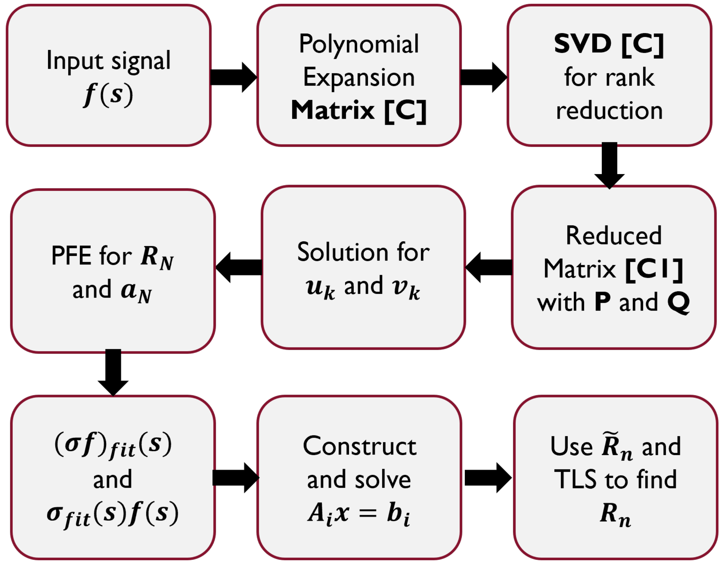
which is again solved as a least square problem. Reconstructing the signal with residues $c_n$, the poles ${\tilde{c}}_N$, d, and $sh$, and comparing it to the input signal gives us the validation for the CNRs calculated here. We include an overview of the method in Figure 1.

3. Backscattering Scenarios

To validate the results of the VCM and also carry out a comparison with the regular and most updated Cauchy Method from [9], a set of simulated and experimental signals were constructed. The idea is to compare the fidelity of the reconstruction of both methods by the Feature Selective Validation (FSV) approach [14]. FSV, proposed by Duffy et al., is used for the comparison of electromagnetic compatibility signals, as it would be executed by expert engineers.

The reconstruction of the input signal using each CNRs’ extraction method uses the complete set of poles and residues extracted and has no manual CNR selection process as the intention is to automate these algorithms as much as possible.

For this reason, the plots in the complex plane also contain resonances that could be considered as errors, because they are not complex conjugated, out of range, or in the positive and real part of the complex plane.

3.1. Simulation

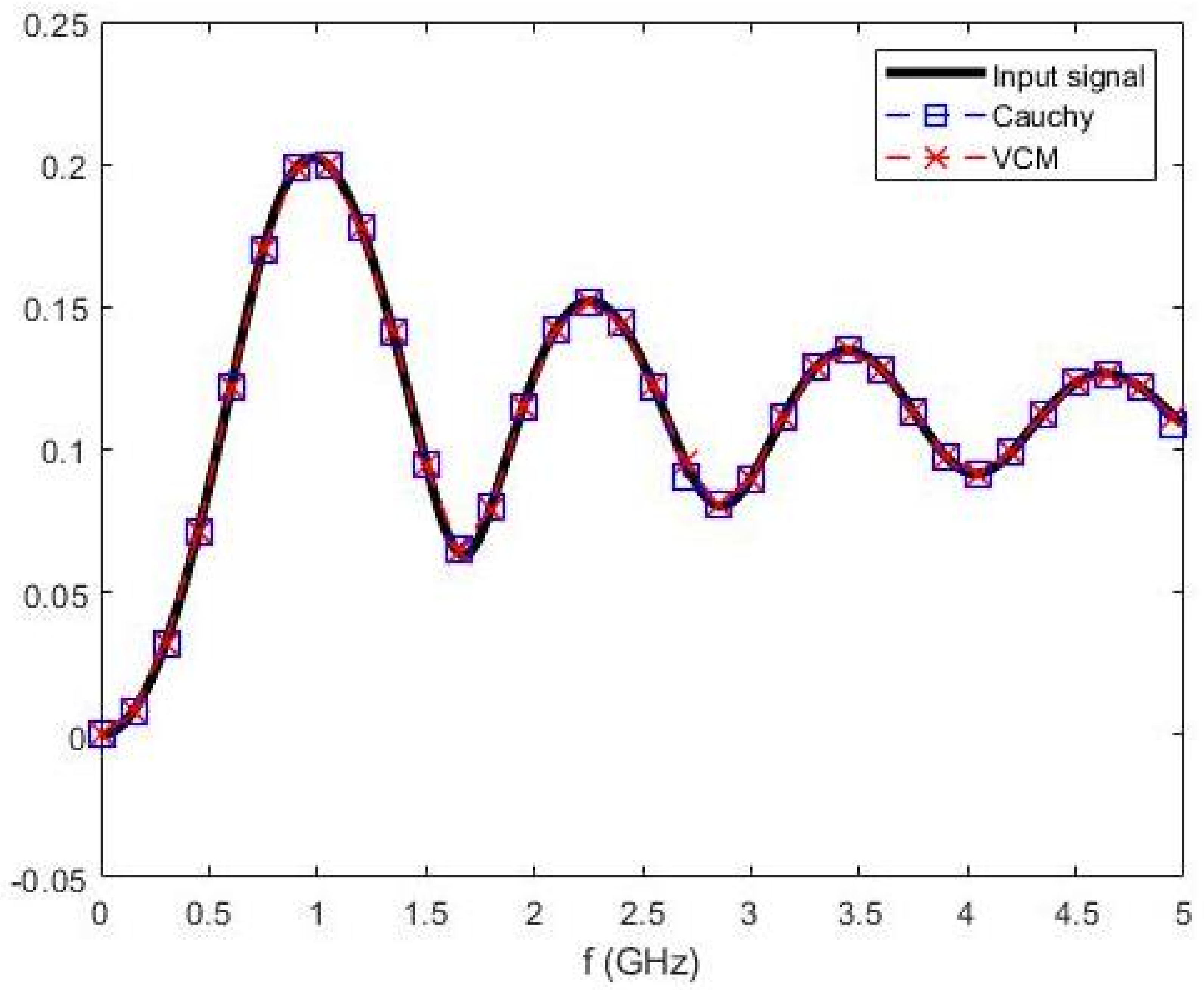
Backscattering scenarios were simulated in CST Microwave Studio to obtain the frequency response signals processed afterward with the Cauchy and VCM methods. A perfectly conducting thin wire, sphere, plate, and cylinder were used as canonical objects, illuminated with a plane wave and placing electric field probes in different positions. An example of the simulated backscattering signals of a metal sphere and the comparison of its reconstructions are presented in Figure 2. Here, the difference in the input signal for both approximations is small compared to the dimension of the data; however, it is calculated using FSV.

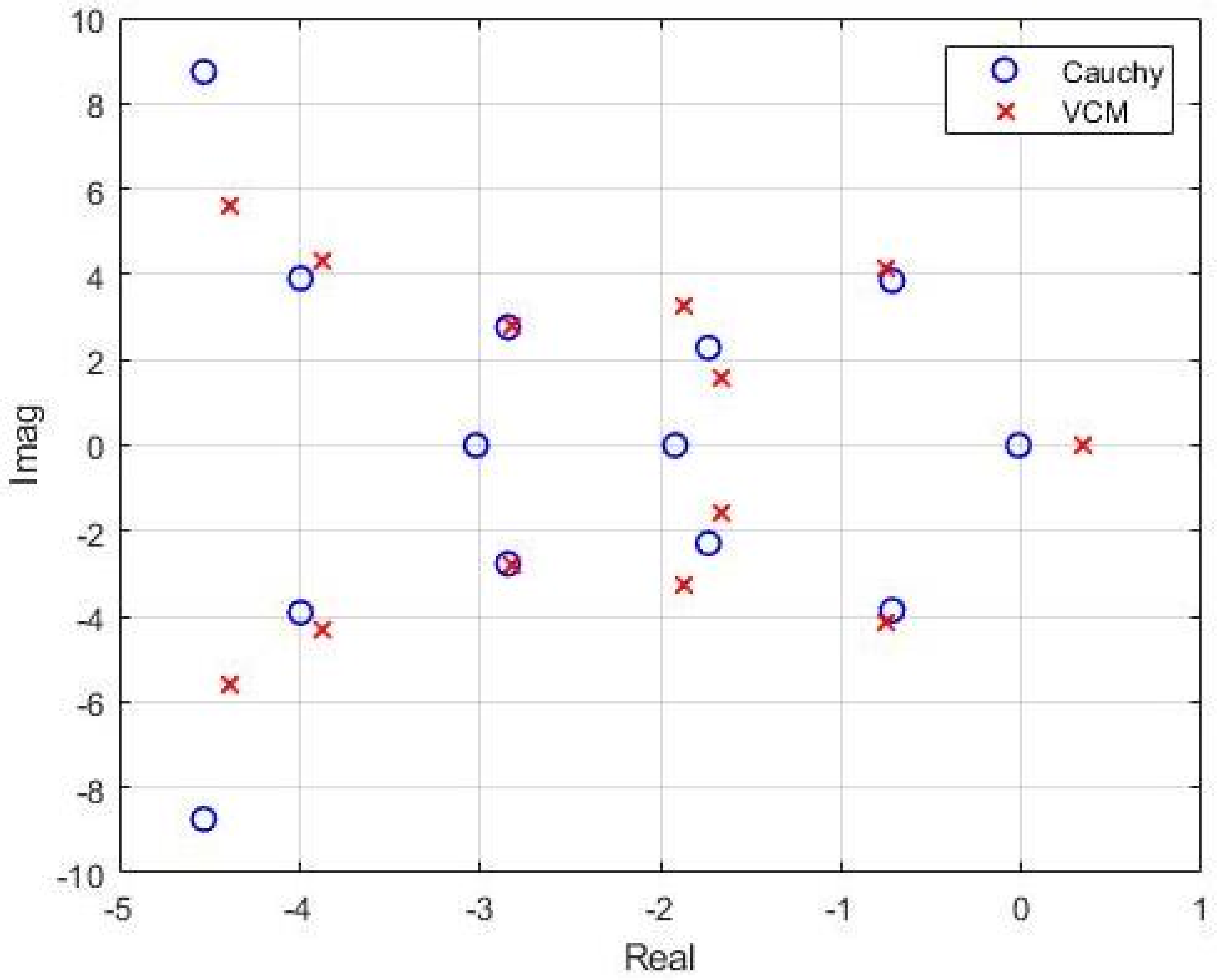
On the other hand, the set of CNRs calculated for this scenario is presented in Figure 3, where the pole shifting in VCM leads to changes in the reconstructed signal.

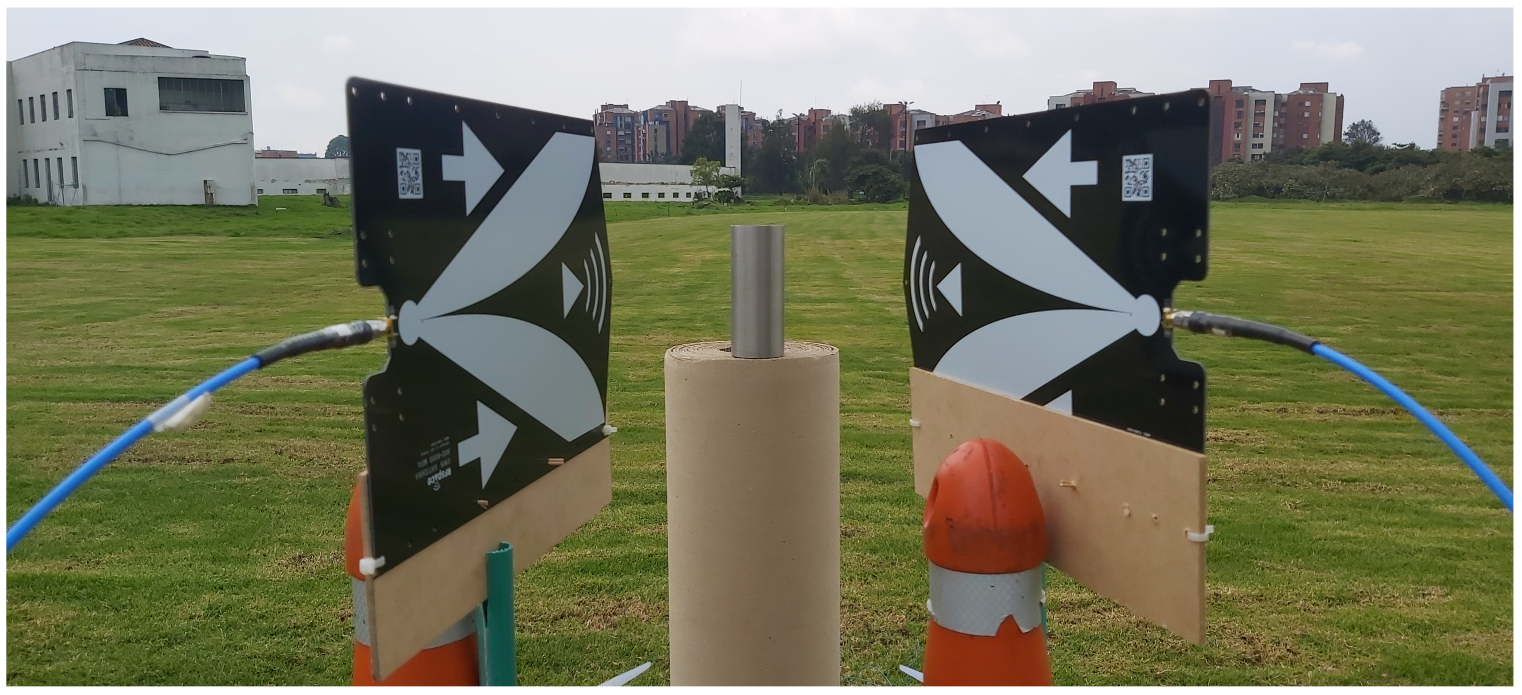
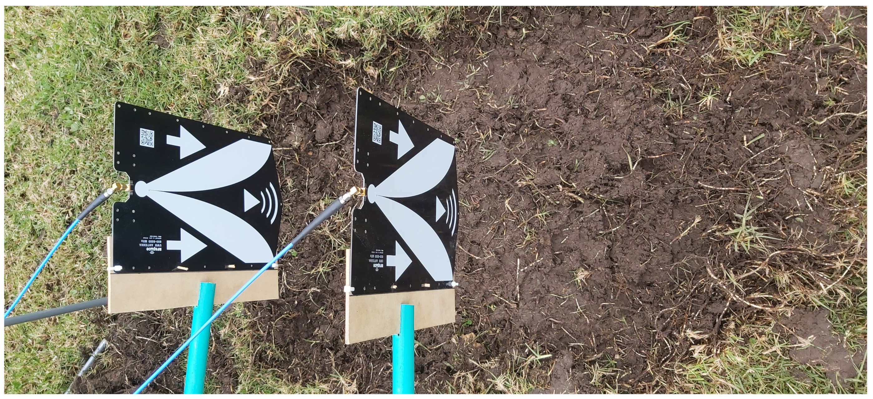
3.2. Experimental

A corner reflector, a cylinder, and a detonator frequently used in the manufacturing of Improvised Explosive Devices (IEDs) in Colombia were the metallic objects used for the two experimental setups. The frequency response was obtained using a VNA up to 3 GHz for free space and up to 6 GHz for the buried scenarios, two TSA600 Vivaldi antennas, and three distances from the source to the object. Furthermore, clutter, antenna coupling, and the background for the experimental signals were removed using the GPR signal acquisition methodology presented in [15].

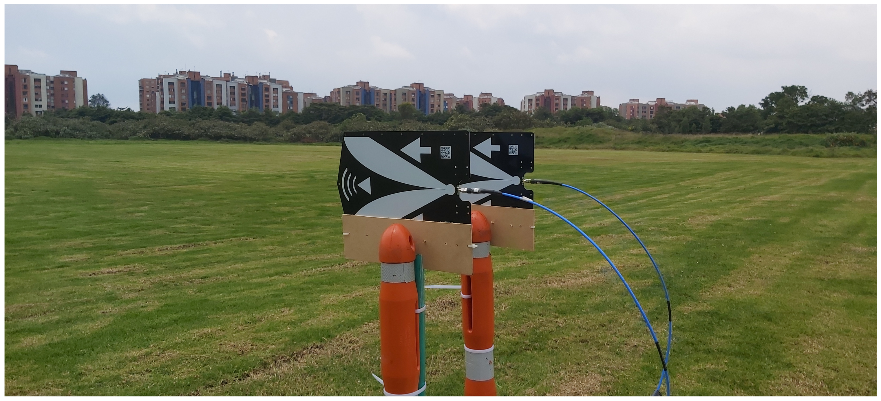
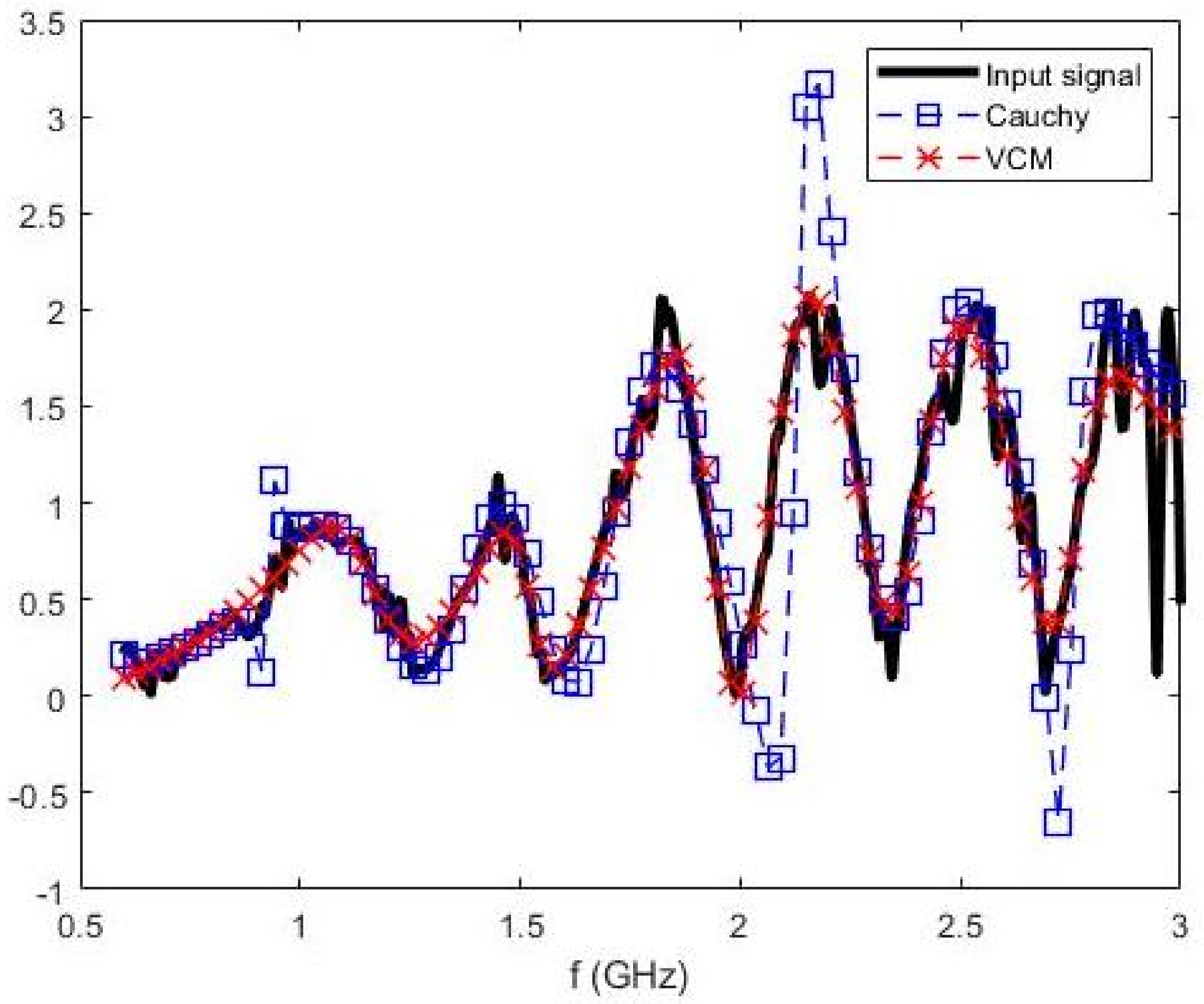
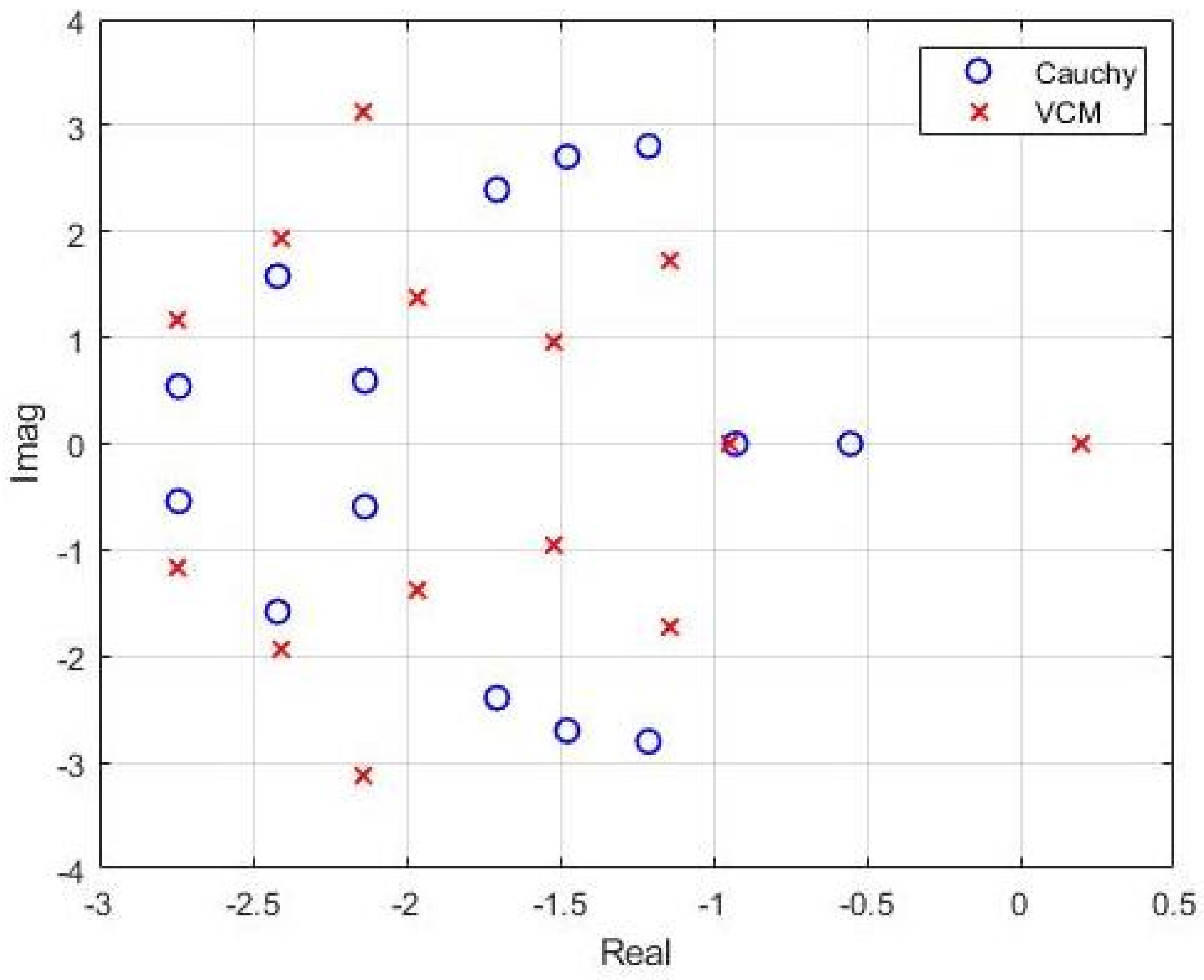
Figure 4 and Figure 5 show the experimental configuration for the metal cylinder in free space, Figure 6 shows an example of the reconstructed signals in the frequency domain, and Figure 7 shows the calculated CNRs in the complex plane. The difference in the reconstructed signals and poles location between Cauchy and VCM becomes more evident in the experimental signals, and it was again calculated using FSV. The difference in the reconstructions for the frequency domain input signals using Cauchy and VCM methods was evaluated with FSV. The curves appear to be similar, but only the numerical evaluation will provide a real comparison, as in Section 4. Again, the SVD-based system order calculation and linearized problem solution can be treated as in [16].

Now, in the experimental setup for buried objects, the same antennas were used, this time targeting the objects buried 15 cm. Figure 8 and Figure 9 present the configuration. Both experiments included IED detonators used in Colombia; the one used here is shown in Figure 10 with an approximate dimension of 54 mm.

Again, as an example of the results to be shown in the next section, the backscattered frequency domain signal for the metal detonator and its associated CNRs for both the Cauchy and VCM methods are displayed in Figure 11 and Figure 12.

The CNR of the highest frequency (imaginary part) for VCM in the complex plane represents a more accurate length of the detonator.

4. Results and Comparison

Among the simulations and experiments, 30 signals were obtained, each one processed with VCM to calculate the corresponding CNRs of a metallic object. After this, FSV provided us with a numerical value for the comparison between the reconstruction and the input signal, as shown in

Table 1. Categories for the similarity of the two signals according to the FSV results.

FSV Categories for Result Value v
Excellent	$vs.<=0.1$
Very good	$0.1<vs.<=0.2$
Good	$0.2<vs.<=0.4$
Fair	$0.4<vs.<=0.8$
Poor	$0.8<vs.<=1.6$
Extremely poor	$v>1.6$

. The execution time in MATLAB 2021a using a core i7 computer with 12 GB RAM and the number of samples used are also shown in the results for the simulation setups in

Table 2. Simulated scenarios’ FSV results for VCM, with execution time and the number of samples used.

		FSV	# of Samples	Execution Time (ms)
Simulation	Thin-Wire	0.001	37	98.5
		0.001	37	99.7
		0.002	37	118.9
	Cylinder	0.063	21	95.3
		0.041	21	95.7
		0.014	21	92
	Plate	0.0001	21	95.8
		0.0002	21	94.8
		0.0004	21	97.3
	Sphere	0.02	37	102
		0.077	37	122.1
		0.037	37	105.6
	Average	0.021	29	101

. As the signal became more complex, the CNR extraction method reduced its accuracy. This means that the resonances of the object were less valid for postprocessing and analysis.

The average FSV for the simulated signals was 0.021, which classifies the reconstruction with VCM in these scenarios as Excellent. For the experimental signals, the results are shown in

Table 3. Free space and buried objects scenarios’ FSV results for VCM, with execution time and the number of samples used.

			FSV	# of Samples	Execution Time (ms)
Experimental Scenarios	Free Space	Corner Reflector	0.18	37	96.07
			0.076	37	97.2
			0.121	37	97.2
		Metal cylinder	0.124	37	171.7
			0.119	37	99.1
			0.164	37	103.6
		Detonator	0.171	37	103.3
			0.155	37	98.8
			0.111	37	107.2
	Buried objects	Corner reflector	0.275	30	100.2
			0.262	30	98
			0.277	30	99.3
		Metal cylinder	0.381	30	99.8
			0.329	30	100.4
			0.204	30	104.2
		Detonator	0.322	30	101.1
			0.126	30	106.1
			0.183	30	98.4
	Average		0.199	34	105

, where the average FSV result was 0.1989 being classified in the Very Good category.

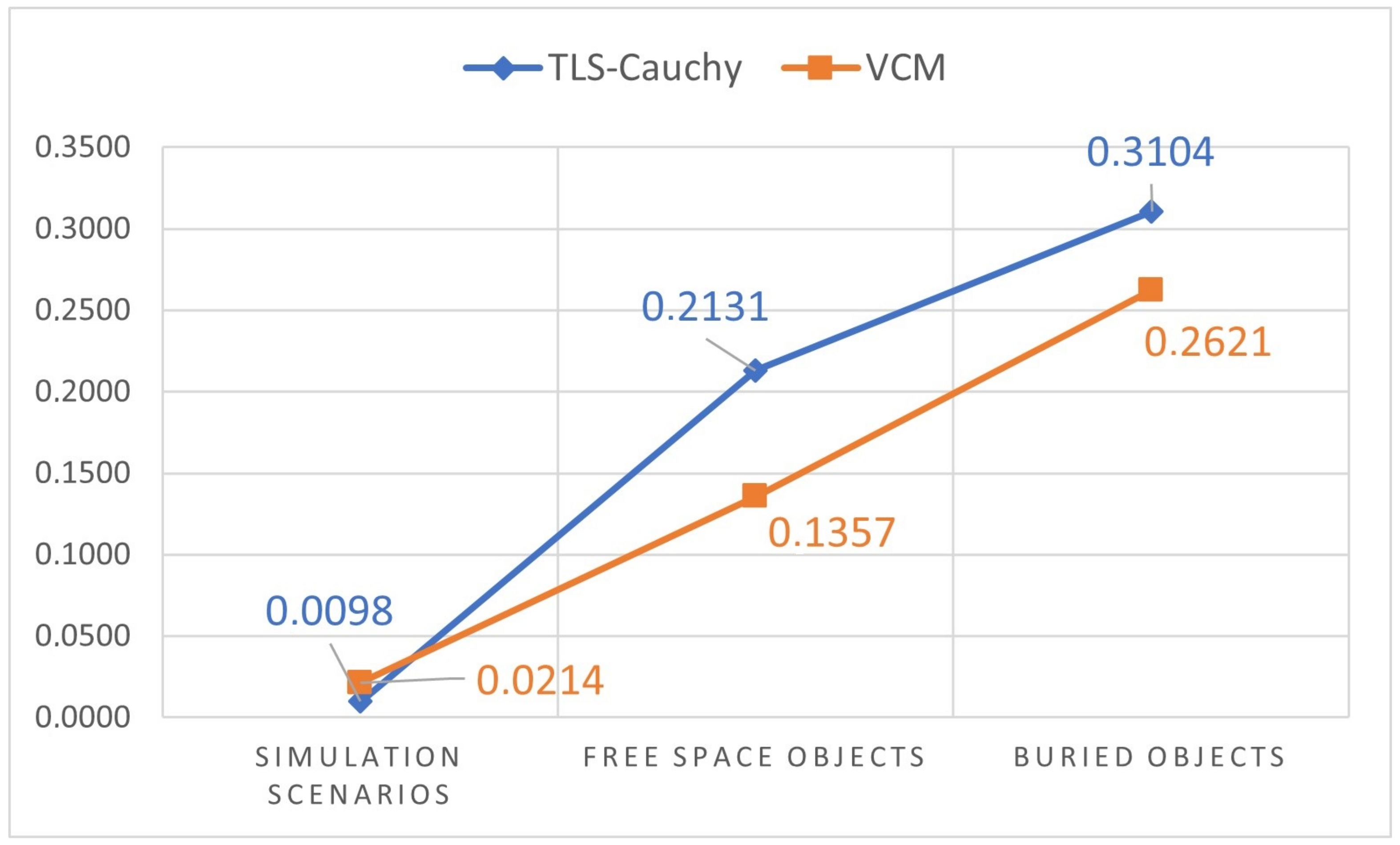
Now, although the validation in the simulated and experimental scenarios resulted in a Very Good reconstruction on average, we also compared the VCM results against the Cauchy method, which is the most updated frequency domain CNR calculation method used in GPR. The average FSV result for the Cauchy method was 0.161, while for VCM it was 0.128. Furthermore, in Figure 13, the values of the FSV result for each scenario are shown.

Here, the Cauchy method outperformed in execution time for all backscattered signals with an average of 61 ms, while for VCM, it was 103 ms. In addition, the reconstruction accuracy for the simulated scenarios was also better in the Cauchy method by 0.0116 in the FSV factor. For all experimental setups, the VCM’s FSV factor was always below Cauchy’s, having a more accurate reconstruction; hence, its CNRs’ extracted were more reliable in these scenarios by 24.2%.

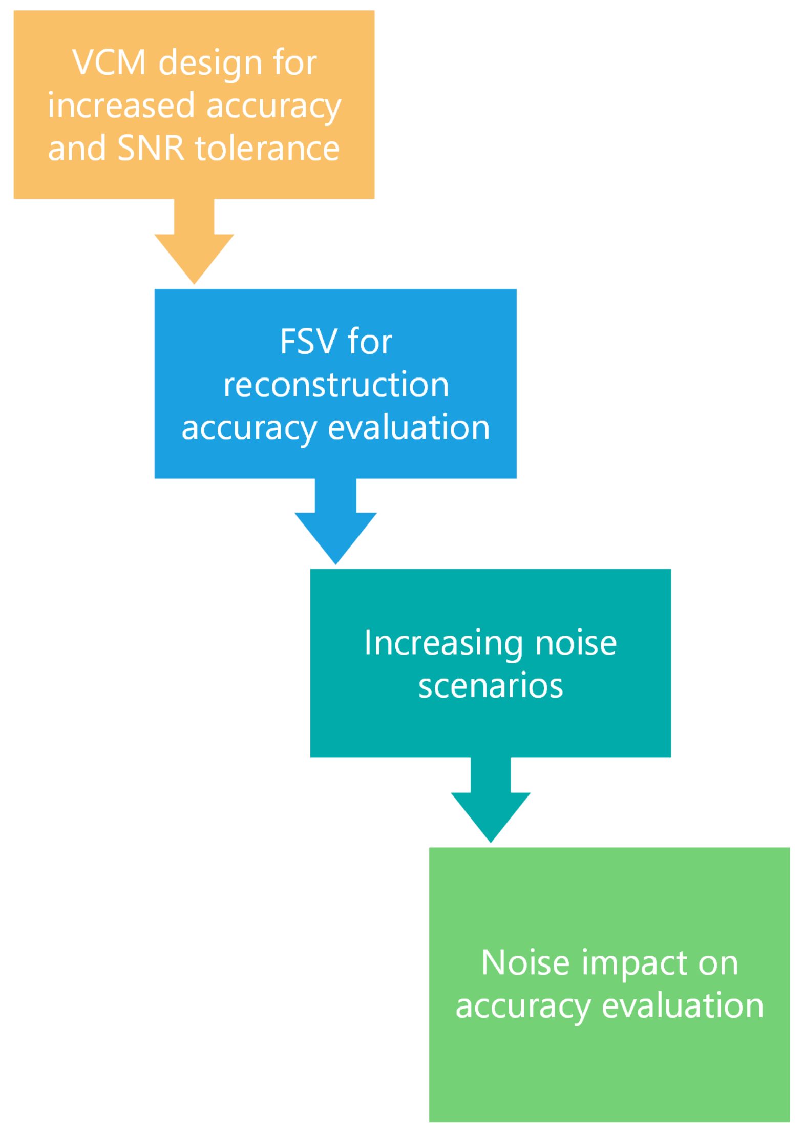
As the accuracy of the reconstructed signal, i.e., the accuracy of the CNRs calculated with previous frequency domain methods is considerably affected by noise, the VCM algorithm was designed. An evaluation of the similarity between the input and the reconstructed signal (FSV) and increasing noise scenarios demonstrated the increased signal-to-noise tolerance of VCM and were used for a noise impact evaluation. Figure 14 summarizes these concepts.

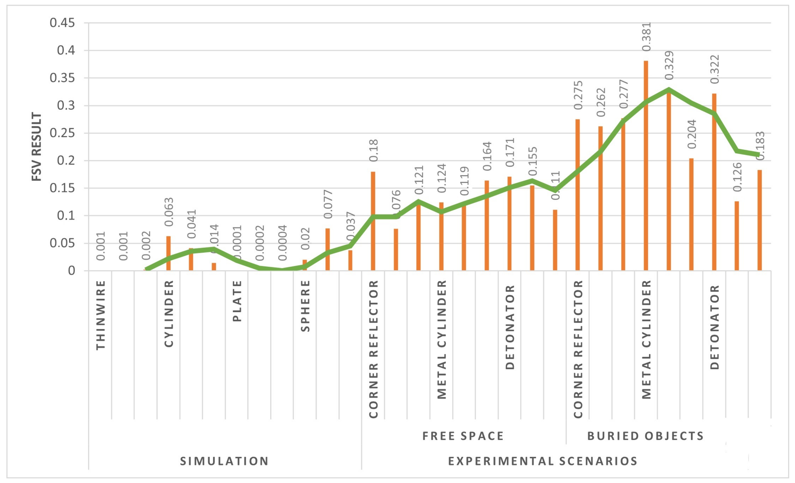
The FSV results data from all scenarios, starting with the simulations, then the free space, and then the buried samples, are considered to have a decreasing SNR, i.e., the backscattering response of interest hides in the response noise as the scenario becomes more complex. If we arrange the information in this manner, an understanding of how well this CNR extraction algorithm performs as noise increases is displayed in Figure 15.

Here, the FSV result increasing alongside the noise and the green line corresponding to a moving average suggest that the signal recovery diminishes in precision as the SNR decreases. This agrees with Dudley in [8], which stated that only approximations to resonances in lossy mediums with frequency-dependent attenuation are ever available in the limits of vanishing noise.

5. Conclusions and Future Work

Here, we presented the Vector Fitting–Cauchy Method (VCM) and validation of the CNRs calculated with frequency-domain methods using FSV. These preliminary results show an advantageous procedure for calculating more reliable resonances from backscattered signals originating from buried objects. As the SNR and the effects on recovery are critical, VCM provides an alternative to previous CNR extraction methods for object recognition. More experiments in different soils will provide a better insight into its behavior in different soil conditions that emulate the landmine context in Colombia. These GPR operations for identifying IEDs is of high interest, and this method, alongside other SEM approaches, are currently being studied and used.

The CNR reliability increase, coming from the validation with FSV and the more accurate pole locations, show a better reconstruction of the signals, and the VCM can be improved in the future by refining the general procedure and reducing the numerical noise in all the matrix operations.

References

- Baum, C.E. On the Singularity Expansion Method for the Solution of Electromagnetic Interaction Problems; Technical Report; Air Force Weapons Lab: Kirtland AFB, NM, USA, 1971. [Google Scholar]
- Baum, C.E.; Rothwell, E.J.; Chen, K.M.; Nyquist, D.P. The Singularity Expansion Method and Its Application to Target Identification. Proc. IEEE 1991, 79, 1481–1492. [Google Scholar] [CrossRef]
- Baum, C.E. The Singularity Expansion Method: Background and Developments. IEEE Antennas Propag. Soc. Newsl. 1986, 28, 14–23. [Google Scholar] [CrossRef]
- Caboussat, A.; Miers, G.K. Numerical approximation of electromagnetic signals arising in the evaluation of geological formations. Comput. Math. Appl. 2010, 59, 338–351. [Google Scholar] [CrossRef] [Green Version]
- Drissi, K.E.K. The Matrix Pencil method applied to smart monitoring and radar. Comput. Methods Exp. Meas. XVII 2015, 59, 13–24. [Google Scholar] [CrossRef] [Green Version]
- Alexopoulos, A.; Drakopoulos, G.; Kanavos, A.; Mylonas, P.; Vonitsanos, G. Two-Step Classification with SVD Preprocessing of Distributed Massive Datasets in Apache Spark. Algorithms 2020, 13, 71. [Google Scholar] [CrossRef] [Green Version]
- Gallego, A.; Pineda, E.; Gutierrez, S.; Román, F. Complex Natural Resonances extraction methods for Ground Penetrating Radar operations. Digit. Signal Process. 2022. Manuscript submitted for publication. [Google Scholar]
- Dudley, D. Progress in identification of electromagnetic systems. IEEE Antennas Propag. Soc. Newsl. 1988, 30, 5–11. [Google Scholar] [CrossRef]
- Lee, W.; Sarkar, T.K.; Moon, H.; Salazar-Palma, M. Computation of the natural poles of an object in the frequency domain using the cauchy method. IEEE Antennas Wirel. Propag. Lett. 2012, 11, 1137–1140. [Google Scholar] [CrossRef]
- Adve, R.; Sarkar, T. The effect of noise in the data on the Cauchy method. Microw. Opt. Technol. Lett. 1994, 7, 242–247. [Google Scholar] [CrossRef]
- Gustavsen, B.; Semlyen, A. Rational Approximatin of Frequency Domain Responses by Vector Fitting. IEEE Trans. Power Deliv. 1999, 14, 1052–1061. [Google Scholar] [CrossRef] [Green Version]
- Gustavsen, B. Improving the pole relocating properties of vector fitting. IEEE Trans. Power Deliv. 2006, 21, 1587–1592. [Google Scholar] [CrossRef]
- Gallego, A.; Vega, F.; Rangel, A. Hybrid Method for the Estimation of Complex Natural Resonances using Cauchy and Vector Fitting. In Proceedings of the 2020 IEEE International Conference on Computational Electromagnetics (ICCEM), Singapore, 24–26 August 2020; pp. 69–71. [Google Scholar]
- Duffy, A.P.; Martin, A.J.; Orlandi, A.; Antonini, G.; Benson, T.M.; Woolfson, M.S. Feature selective validation (FSV) for validation of computational electromagnetics (CEM). part I-the FSV method. IEEE Trans. Electromagn. Compat. 2006, 48, 449–459. [Google Scholar] [CrossRef]
- Lambot, S.; Slob, E.C.; van den Bosch, I.; Stockbroeckx, B.; Vanclooster, M. Modeling of ground-penetrating radar for accurate characterization of subsurface electric properties. IEEE Trans. Geosci. Remote Sens. 2004, 42, 2555–2568. [Google Scholar] [CrossRef]
- Liseno, A.; Pierri, R. Imaging perfectly conducting objects as support of induced currents: Kirchhoff approximation and frequency diversity. J. Opt. Soc. Am. Opt. Image Sci. Vis. 2002, 19, 1308–1318. [Google Scholar] [CrossRef] [PubMed]
Figure 1.
General steps in the VCM algorithm to find CNRs from a frequency domain signal. A reconstructed signal could be compared to the input one for validation purposes.
Figure 2.
Metal sphere signal approximation using the Cauchy and VCM methods.
Figure 3.
CNRs calculated with the Cauchy and VCM methods for a simulated metal sphere.
Figure 4.
Free space experimental setup with no objects.
Figure 5.
Free space experimental setup with a metal cylinder.
Figure 6.
Frequency domain backscattered signal obtained from a metal cylinder in free space at 60 m.
Figure 7.
CNRs calculated with Cauchy and VCM that were used to reconstruct the backscattered signals of the metal cylinder in free space.
Figure 8.
Buried objects experimental setup, soil alone.
Figure 9.
Buried objects experimental setup with a metal IED detonator.
Figure 10.
Electric IED detonators commonly used in Colombia. The approximate dimension is 54 mm, with a diameter of 4 mm.
Figure 11.
Backscattering signal reconstruction with the Cauchy and VCM methods corresponding to an electric metal detonator for IEDs in Colombia.
Figure 12.
CNRs calculated with both the Cauchy and VCM methods using the frequency response of an electric metal detonator for IEDs in Colombia.
Figure 13.
FSV results for both the Cauchy and VCM methods, according to the comparison of the input signals and the corresponding reconstruction in the simulated and experimental setups.
Figure 14.
Summary of the signal-to-noise tolerance improvement and evaluation.
Figure 15.
FSV result for all backscattering scenarios arranged according to increasing signal noise. The green line corresponds to a moving average and is higher for buried objects scenarios.