The Efficient Processing of Moving k-Farthest Neighbor Queries in Road Networks ^†

Abstract

Given a set of facilities F and a query point q, a k-farthest neighbor (kFN) query returns the k farthest facilities $f_1,f_1,\cdots ,f_k$ from q. This study considers the moving k-farthest neighbor (MkFN) query that constantly retrieves the k facilities farthest from a moving query point q in a road network. The main challenge in processing MkFN queries in road networks is avoiding the repeated retrieval of candidate facilities as the query point arbitrarily moves along the road network. To this end, this study proposes a moving farthest search algorithm (MOFA) to compute valid segments for the query segment in which the query point is located. Each valid segment has the same k facilities farthest from the query locations in the valid segment. Therefore, MOFA retrieves candidate facilities only once for the query segment and computes valid segments using these candidate facilities, thereby avoiding the repeated retrieval of candidate facilities when the query point moves. An empirical study using real-world road networks demonstrates the superiority and scalability of MOFA compared to a conventional solution.

1. Introduction

Given a positive integer k, query point q, and set of facilities F, the k-farthest neighbor (kFN) query retrieves the k facilities farthest from the query point q, whereas the k-nearest neighbor (kNN) query retrieves the k facilities closest to the query point q. kFN queries are the logical opposite of kNN queries. This study considers moving k-farthest neighbor (MkFN) queries in road networks. MkFN queries constantly retrieve the k facilities farthest from a moving query point q. The kFN search has real-world applications, including computational geometry, artificial intelligence, pattern recognition, and information retrieval methods [1,2,3,4,5,6,7,8,9,10,11,12]. A farthest neighbor (FN) search specifically determines the smallest radius of a circle centered on a point q that covers all facilities. Consider a real-world scenario involving a team of commandos on a mission in which the leader requests that no member of the team should be more than 1 km away from him. Naturally, the leader should pay close attention to the farthest team members to monitor their activities and ask them not to move too far away. As another example of the FN search, locating obnoxious facilities such as waste incinerators is often performed in a manner that will maximize the distance between residential areas and these facilities.

Given a positive integer $k=2$, the moving query point q, and set of five facilities $F=\{f_1,f_2,f_3,f_4,f_5\}$ (Figure 1), the MkFN query should constantly retrieve the two facilities farthest from the moving query point q in the road network. Suppose that the query point q locations at timestamps $t_1$ and $t_2$ are represented by $q_{t_1}$ and $q_{t_2}$, respectively. $f_1$ and $f_2$ are the two facilities farthest from $q_{t_1}$, and $f_4$ and $f_5$ are the two facilities farthest from $q_{t_2}$. A simple solution for MkFN queries in road networks involves computing the network distance from a query point q to each facility f in F. An additional $O\left(\right|F|·\log \left|F\right|)$ time is required to retrieve the k facilities farthest from q. However, this simple solution cannot be used in practical applications because kFN queries should be regularly evaluated to refresh the query results while q moves continuously. Therefore, this study proposes a moving farthest search algorithm called MOFA that enables the efficient evaluation of MkFN queries in road networks. MOFA computes the valid segments for the query segment in which the query point q moves such that it does not repeatedly retrieve candidate facilities whenever q moves. To this end, MOFA quickly retrieves the candidate facilities for the query segment and computes the valid segments using the candidate facilities. Each query location in the valid segment has the same k facilities farthest from the query location.

Figure 2 presents an example of an MkFN query, where q moves along query segment $\overline{q_s{q}_{\mathrm{e}}}$. First, the moving query point q submits a query segment $\overline{q_s{q}_{\mathrm{e}}}$ to the location-based service (LBS) server, instead of the current q location. Next, the LBS server returns a set of valid segments for $\overline{q_s{q}_{\mathrm{e}}}$, where each valid segment has the same k facilities farthest from each query location in the valid segment. This study assumes that query points (e.g., vehicles and pedestrians) move, while facilities (e.g., garbage incinerators and chemical plants) are stationary. To the best of our knowledge, this is the first attempt to study the efficient processing of MkFN queries in road networks.

The main contributions of this study are summarized below.

• This study proposes MOFA to compute valid segments for the query segment in which a query point moves.
• MOFA retrieves candidate facilities once and has a stable query processing time that is independent of the query frequency.
• An extensive empirical evaluation is performed using real-world road networks to demonstrate the superiority of MOFA compared to a conventional solution.

The remainder of this paper is organized as follows. Section 2 reviews the related research. Section 3 describes the MkFN query problem and notation used in this study. Section 4 describes the clustering of facilities and calculation of distances between facility clusters and a border point. Section 5 presents MOFA for MkFN query processing in road networks, and Section 6 evaluates an example of MkFN query using MOFA. Section 7 presents the empirical results obtained using MOFA and conventional algorithms with different setups, and Section 8 summarizes our conclusions.

2. Related Works

Many studies have been conducted on the efficient processing of spatial queries based on the FN search [1,2,3,4,5,6,7,8,9,10,11,12].

• Reverse FN (RFN) query [3,4,5,7,8,9,13]. Given a set of facilities F and a query point q, an RFN query retrieves the facilities in F that have q as their farthest neighbor. Recently, RFN queries have attracted increasing attention based on their applicability. Several studies have been conducted to efficiently evaluate RFN queries in Euclidean spaces [3,4,8,9,13] and road networks [5,7].
• Approximate FN query [1,10,11,14]. Given an approximation ratio c ($c>1$) and success probability $\delta$, a c-approximate FN query retrieves the c-approximate farthest neighbors with a confidence of at least $\delta$. Approximate FN search algorithms are considered acceptable in high-dimensional spaces because it is typically not feasible to return the exact farthest neighbors in a large set of points. Huang et al. [10,14] developed a reverse-query-aware locality-sensitive hashing scheme for high-dimensional c-approximate FN searches over external memory. They also proposed a heuristic variant that applied data-dependent object selection to reduce the number of data objects. Liu et al. [11] proposed a c-approximate FN algorithm called reverse incremental locality-sensitive hashing for high-dimensional data that employs a continuous search strategy for each projection dimension.
• Aggregate FN query [2,6]. Given a set of query points Q and an aggregate function (e.g., min, max, and sum), the aggregate FN query retrieves a facility f from a set of facilities F such that the aggregate distance from f to all query points in Q is maximized. Gao et al. [2] studied the aggregate FN query in Euclidean space and proposed the smallest-bounding and best-first algorithms. Wang et al. [6] presented effective solutions to aggregate FN queries in road networks.
• Moving spatial query [15,16,17,18]. Various types of moving spatial queries have been studied extensively, including kNN [15,16,17] and range [18] queries. Nutanong et al. [17] developed an incremental safe region-based technique known as the $V^{*}$-diagram to process moving kNN queries in Euclidean space and in undirected spatial networks. Yung et al. [18] proposed an algorithm for computing the boundaries, which are referred to as safe exits, of the safe regions of moving-range queries in road networks. The associated studies considered different problem scenarios from those in our study, and their solutions were found to be inappropriate for our problem scenarios.

Spatial access methods based on Euclidean distance cannot process MkFN queries in road networks because network distance evaluation is much more expensive than Euclidean distance evaluation. Solutions for the MkNN search [15,16,17] are not applicable to MkFN query settings because MkFN queries focus on the farthest neighbors, rather than the nearest neighbors. This is an extended version of a preliminary conference report presented at the KSCI Summer Conference 2021 [19]. The preliminary conference report [19] describes the key concepts of MOFA without empirical evidence. Therefore, in this study, MOFA was thoroughly analyzed and an empirical evaluation was performed. This study also differs from our previous studies [20,21] in several aspects. Cho [20] considered kFN join queries in a spatial network. The kFN join query focuses on evaluating a snapshot of the kFN query for each query point in Q. Cho and Attique [21] presented the group processing of multiple kFN (GMP) algorithms to efficiently process multiple kFN queries in road networks. The GMP algorithm exploits shared computation techniques to rapidly process snapshot kFN queries for multiple query points with distinct query conditions. Unlike our previous studies [20,21] on snapshot kFN queries, this study focuses on computing valid segments for continuous kFN queries of a moving query point.

Table 1. Comparison between our problem scenario and those of previous studies.

References	Space Domain	Query Type
[3,4,8,9,13]	Euclidean space	Reverse FN query
[1,4,10,11,12,14]	Euclidean space	FN query
[2]	Euclidean space	Aggregate FN query
[5,7]	Road network	Reverse FN query
[6]	Road network	Aggregate FN query
[20]	Road network	FN join query
[21]	Road network	Multiple FN query
This study	Road network	Moving FN query

compares our problem scenario with those in previous studies to identify the differences between them.

3. Notation and Formal Problem Description

Definition 1.

kFN query [1,2,3,4,5,6,7,8]. Given a set of facilities F, positive integer k, and query point q, the query point q retrieves the set of k facilities farthest from q, which is denoted as $\mathrm{\Phi }\left(q\right)$.

Definition 2.

MkFN query. Given a set of facilities F, positive integer k, and moving query point q, the moving query point q constantly retrieves the set of k facilities farthest from q. We assume that $\overline{q_s{q}_e}$ is a query segment in which q moves. Then, the MkFN query result can be represented as $\mathrm{\Phi }\left(\overline{q_s{q}_e}\right)=\left\{〈q,\mathrm{\Phi }\left(q\right)〉\right|q\in \overline{q_s{q}_e}\}$.

Definition 3.

Road network and network distance [22,23,24,25,26]. A road network G is modeled as a weighted undirected graph $G=〈V,E,W〉$, where V is a set of road intersections, E is a set of road segments, and W represents the distance matrix. The network distance $d(q,f)$ between q and f, where q and f are two points on G, is the sum of the lengths of the road segments along the shortest path between q and f. The terms “network distance” and “length of the shortest path” are used interchangeably.

4. Clustering Facilities and Computing Distances

Section 4.1 discusses grouping nearby facilities into clusters. Section 4.2 discusses calculating the largest and smallest distances from the border point of the query segment to a facility cluster.

4.1. Clustering Facilities into Facility Clusters

Figure 3 presents an example MkFN query q, where $k=2$ and $F=\{f_1,f_2,\cdots ,f_6\}$. This example is used to elaborate the solution process. The example MkFN query requires that the moving query point q constantly retrieves the two facilities farthest from itself. The vertex list in which query point q moves is referred to as the query segment for q. In this example, $\overline{v_1{v}_2}$ is the query segment for q (Figure 3). For ease of identification, the query segment is shown in bold.

Figure 4 illustrates the segmentation of a road network. In this figure, the intersection vertices corresponding to road intersections are marked using dashed circles. The example road network contains six intersection vertices $v_1$, $v_2$, $v_3$, $v_4$, $v_5$, and $f_5$. The degrees are represented by numbers in parentheses. In this study, a road network is split into vertex lists using intersection vertices. Therefore, facility segments adjacent to an intersection vertex are grouped into a facility cluster, as illustrated in Figure 5.

Figure 5 illustrates the clustering method for grouping facilities into facility clusters. The clustering method first groups facilities in a vertex list into a facility segment. Adjacent facility segments are then grouped into a facility cluster. First, the facilities $f_1$, $f_2$, and $f_3$ in a vertex list $\overline{v_3{f}_2{v}_5}$ are connected to form a facility segment $\overline{f_1{f}_2{f}_3}$. Similarly, the facilities $f_4$ and $f_5$ in the vertex list $\overline{f_5{v}_4}$ are connected to form a facility segment $\overline{f_4{f}_5}$. Therefore, there are three facility segments $\overline{f_1{f}_2{f}_3}$, $\overline{f_4{f}_5}$, and $f_6$ (Figure 5a). Next, the two facility segments $\overline{f_4{f}_5}$ and $f_6$ are connected using the intersection vertex $f_5$ to form a facility cluster $\{\overline{f_4{f}_5},\overline{f_5{f}_6}\}$. Therefore, a set of facilities $F=\{f_1,f_2,\cdots ,f_6\}$ changes into a set of facility clusters $\overline{F}=\{\left\{\overline{f_1{f}_2{f}_3}\right\},\{\overline{f_4{f}_5},\overline{f_5{f}_6}\}\}$. In the proposed method, facility segments constitute a facility cluster, which is represented by a set of facility segments.

4.2. Computing Distances between a Facility Cluster and a Border Point of the Query Segment

The largest and smallest distances between a facility cluster $\overline{F_C}$ and a border point $q_b$ of the query segment $\overline{q_{\mathrm{s}}{q}_{\mathrm{e}}}$ are computed, where $q_b\in \{q_s,q_e\}$. The smallest and largest distances between $\overline{F_C}$ and $q_b$ are represented by $d_{min}(q_b,\overline{F_C})=min\left\{d(q_b,f)\right|f\in \overline{F_C}\}$ and $d_{max}(q_b,\overline{F_C})=max\left\{d(q_b,f)\right|f\in \overline{F_C}\}$, respectively. The smallest distance between $q_b$ and $\overline{F_C}$ is evaluated as $d_{min}(q_b,\overline{F_C})=min\left\{d(q_b,f_b)\right|f_b\in B\left(\overline{F_C}\right)\}$, where $f_b$ is a border point of $\overline{F_C}$. However, the largest distance between $q_b$ and $\overline{F_C}$ is evaluated as $d_{max}(q_b,\overline{F_C})=max\left\{d_{max}(q_b,\overline{f_l{f}_m})\right|\overline{f_l{f}_m}\in \overline{F_C}\}$, where $\overline{f_l{f}_m}$ is a facility segment in $\overline{F_C}$, and $d_{max}(q_b,\overline{f_l{f}_m})$ is the largest distance between $q_b$ and $\overline{f_l{f}_m}$.

The largest and smallest distances between a facility cluster $\overline{F_C}$ and a border point $q_b$ of the query segment are computed using the example in Figure 5, where $q_b\in \{v_1,v_2\}$ and $\overline{F}=\{\left\{\overline{f_1{f}_2{f}_3}\right\},\{\overline{f_4{f}_5},\overline{f_5{f}_6}\}\}$. Figure 6, Figure 7, Figure 8 and Figure 9 illustrate the computations of $d_{max}(v_1,\left\{\overline{f_1{f}_2{f}_3}\right\})$, $d_{max}(v_1,\{\overline{f_4{f}_5},\overline{f_5{f}_6}\})$, $d_{max}(v_2,\left\{\overline{f_1{f}_2{f}_3}\right\})$, and $d_{max}(v_2,\{\overline{f_4{f}_5},\overline{f_5{f}_6}\})$, respectively.

Figure 6 depicts the computation of $d_{max}(v_1,\overline{f_1{f}_2{f}_3})$. The distances from $v_1$ to endpoints $f_1$ and $f_3$ of $\overline{f_1{f}_2{f}_3}$ are $d(v_1,f_1)=21$ and $d(v_1,f_3)=21$, respectively, because the path from $v_1$ to $f_1$ ($f_3$) is $v_1\to v_3\to f_1$ ($v_1\to v_2\to v_4\to v_5\to f_3$). Imagine a point f in $\overline{f_1{f}_2{f}_3}$. The distance from $v_1$ to f is then evaluated to $d(v_1,f)$$=min\{d(v_1,f_1)+len\left(\overline{f_{1}f}\right),d(v_1,f_3)+len\left(\overline{f_{3}f}\right)\}$$=min\{21+len\left(\overline{f_{1}f}\right),21+len\left(\overline{f_{3}f}\right)\}$ because the path from $v_1$ to f should be $v_1\to f_1\to f$ or $v_1\to f_3\to f$. Let $x=len\left(\overline{f_{1}f}\right)$. Accordingly, $len\left(\overline{f_{3}f}\right)=5-x$ because $len\left(\overline{f_{1}f}\right)+len\left(\overline{f_{3}f}\right)=5$. The distance from $v_1$ to f can be represented as $d(v_1,f)=min\left\{21+x,21+(5-x)\right\}$ for $0\le x\le 5$. As shown in Figure 6, the largest and smallest distances from $v_1$ to $\overline{f_1{f}_2{f}_3}$ are evaluated as $d_{max}(v_1,\overline{f_1{f}_2{f}_3})=23.5$ and $d_{min}(v_1,\overline{f_1{f}_2{f}_3})=21$, respectively. The star sign (★) in Figure 6 is used to signify $d_{max}(v_1,\overline{f_1{f}_2{f}_3})=23.5$.

Figure 7 illustrates the $d_{max}(v_1,\{\overline{f_4{f}_5},\overline{f_5{f}_6}\})$ computation. Naturally, the largest distance between $v_1$ and $\{\overline{f_4{f}_5},\overline{f_5{f}_6}\}$ is evaluated as $d_{max}(v_1,\{\overline{f_4{f}_5},\overline{f_5{f}_6}\})$ $=max\{d_{max}(v_1,\overline{f_4{f}_5}),$ $d_{max}(v_1,\overline{f_5{f}_6})\}$. Figure 7a,b present the $d_{max}(v_1,\overline{f_4{f}_5})$ and $d_{max}(v_1,\overline{f_5{f}_6})$ computations, respectively. The distance from $v_1$ to $f_4$ ($f_5$) is $d(v_1,f_4)=12$ ($d(v_1,f_5)=8$) because the shortest path from $v_1$ to $f_4$ ($f_5$) is $v_1\to v_2\to f_5\to f_4$ ($v_1\to v_2\to f_5$). Imagine a point f in $\overline{f_4{f}_5}$. The distance from $v_1$ to f is computed as $d(v_1,f)=$$min\{d(v_1,f_4)+len\left(\overline{f_{4}f}\right),d(v_1,f_5)+len\left(\overline{f_{5}f}\right)\}$ $=min\{12+len\left(\overline{f_{4}f}\right),8+len\left(\overline{f_{5}f}\right)\}$; therefore, the largest and smallest distances from $v_1$ to $\overline{f_4{f}_5}$ are calculated as $d_{max}(v_1,\overline{f_4{f}_5})=12$ and $d_{min}(v_1,\overline{f_4{f}_5})=8$, respectively (Figure 7a). The same method in Figure 6 can be used to compute the largest and smallest distances from $v_1$ to $\overline{f_5{f}_6}$ (Figure 7b). The detailed procedure for the largest and smallest distance computation from $v_1$ to $\overline{f_5{f}_6}$ is omitted for simplicity. The shortest path from $v_1$ to $f_5$ ($f_6$) is $v_1\to v_2\to f_5$ ($v_1\to v_2\to f_5\to f_6$), and the distance from $v_1$ to $f_5$ ($f_6$) is $d(v_1,f_5)=8$ ($d(v_1,f_6)=11$). Therefore, the largest and smallest distances between $v_1$ and $\{\overline{f_4{f}_5},\overline{f_5{f}_6}\}$ are computed as $d_{max}(v_1,\{\overline{f_4{f}_5},\overline{f_5{f}_6}\})=12$ and $d_{min}(v_1,\{\overline{f_4{f}_5},\overline{f_5{f}_6}\})=8$, respectively.

Figure 8 demonstrates the $d_{max}(v_2,\overline{f_1{f}_2{f}_3})$ computation. Note that the shortest path from $v_2$ to $f_1$ ($f_3$) is $v_2\to v_4\to v_3\to f_1$ ($v_2\to v_4\to v_5\to f_3$), and the distance from $v_2$ to $f_1$ ($f_3$) is $d(v_2,f_1)=17$ ($d(v_2,f_3)=16$). The same method in Figure 6 can be used to compute the largest and smallest distances from $v_2$ to $\overline{f_1{f}_2{f}_3}$ (Figure 8). The detailed procedure for computing the largest and smallest distances from $v_2$ to $\overline{f_1{f}_2{f}_3}$ is omitted for simplicity. The largest and smallest distances between $v_2$ and $\overline{f_1{f}_2{f}_3}$ are $d_{max}(v_2,\overline{f_1{f}_2{f}_3})=19$ and $d_{min}(v_2,\overline{f_1{f}_2{f}_3})=16$, respectively. The star sign (★) in Figure 8 is used to signify $d_{max}(v_2,\overline{f_1{f}_2{f}_3})=19$.

Figure 9 presents the $d_{max}(v_2,\{\overline{f_4{f}_5},\overline{f_5{f}_6}\})$ computation. The largest distance between $v_2$ and $\{\overline{f_4{f}_5},\overline{f_5{f}_6}\}$ is evaluated as $d_{max}(v_2,\{\overline{f_4{f}_5},\overline{f_5{f}_6}\})$ $=max\{d_{max}(v_2,\overline{f_4{f}_5}),$$d_{max}(v_2,\overline{f_5{f}_6})\}$. Figure 9a,b depict the $d_{max}(v_2,\overline{f_4{f}_5})$ and $d_{max}(v_2,\overline{f_5{f}_6})$ computations, respectively. The distance from $v_2$ to $f_4$ ($f_5$) is $d(v_2,f_4)=7$ ($d(v_2,f_5)=3$) because the shortest path from $v_2$ to $f_4$ ($f_5$) is $v_2\to f_5\to f_4$ ($v_2\to f_5$). The same method in Figure 6 can be used to compute the largest and smallest distances from $v_2$ to $\overline{f_4{f}_5}$ (Figure 9a). Thus, the largest and smallest distances from $v_2$ to $\overline{f_4{f}_5}$ are $d_{max}(v_2,\overline{f_4{f}_5})=7$ and $d_{min}(v_2,\overline{f_4{f}_5})=3$, respectively. The detailed procedure for computing the largest and smallest distances from $v_2$ to $\overline{f_4{f}_5}$ is omitted for simplicity.

The distance from $v_2$ to $f_5$ ($f_6$) is $d(v_2,f_5)=3$ ($d(v_2,f_6)=6$) because the shortest path from $v_2$ to $f_5$ ($f_6$) is $v_2\to f_5$ ($v_2\to f_5\to f_6$). The same method in Figure 6 can be used to compute the largest and smallest distances from $v_2$ to $\overline{f_5{f}_6}$ (Figure 9b). Thus, the largest and smallest distances from $v_2$ to $\overline{f_5{f}_6}$ are $d_{max}(v_2,\overline{f_5{f}_6})=6$ and $d_{min}(v_2,\overline{f_5{f}_6})=3$, respectively. The detailed procedure for computing the largest and smallest distances from $v_2$ to $\overline{f_5{f}_6}$ is also omitted for simplicity. Therefore, the largest and smallest distances between $v_2$ and $\{\overline{f_4{f}_5},\overline{f_5{f}_6}\}$ are $d_{max}(v_2,\{\overline{f_4{f}_5},\overline{f_5{f}_6}\})=7$ and $d_{min}(v_2,\{\overline{f_4{f}_5},\overline{f_5{f}_6}\})=3$, respectively.

5. MOFA Algorithm for MkFN Query Processing in Road Networks

Algorithm 1 presents the MOFA algorithm, which has three steps. The first step groups facilities into facility clusters using the clustering method described in Section 4.1; therefore, a set F of facilities changes to a set $\overline{F}$ of facility clusters. The second step retrieves the candidate facilities for a query segment $\overline{q_s{q}_e}$, which are retrieved from border points $q_s$ and $q_e$. To this end, the $find\_candidates$ function is called from $q_s$ ($q_e$), whose result is stored to $\mathrm{\Sigma }\left(q_s\right)$ ($\mathrm{\Sigma }\left(q_e\right)$). In the third step, the valid segments for $\overline{q_s{q}_e}$ are computed using the candidate facilities in $\mathrm{\Sigma }\left(q_s\right)\cup \mathrm{\Sigma }\left(q_e\right)$. Note that $\mathrm{\Phi }\left(\overline{q_s{q}_e}\right)$ includes valid segments for $\overline{q_s{q}_e}$ and the k facilities farthest from them.

Algorithm 1:$\mathrm{MOFA}(k,\overline{q_s{q}_e},F)$.

Input: k: number of FNs requested for q, $\overline{q_s{q}_e}$: query segment, F: set of facilities Output: $\mathrm{\Phi }\left(\overline{q_s{q}_e}\right)$: query result for $\overline{q_s{q}_e}$, i.e., $\mathrm{\Phi }\left(\overline{q_s{q}_e}\right)=\left\{〈q,\mathrm{\Phi }\left(q\right)〉\right|q\in \overline{q_s{q}_e}\}$ 1: // Step 1: Facilities are grouped into facility clusters, which is explained in Section 4.1. 2: $\overline{F}\leftarrow cluster\_facilities\left(F\right)$ 3: // Step 2: Candidate facilities for $\overline{q_s{q}_e}$ are retrieved by border points, which is detailed in Algorithm 2. 4: $\mathrm{\Sigma }\left(q_s\right)\leftarrow find\_candidates(k,q_s,len\left(\overline{q_s{q}_e}\right),\overline{F})$       //Candidate facilities for $\overline{q_s{q}_e}$ are retrieved by $q_s$. 5: $\mathrm{\Sigma }\left(q_e\right)\leftarrow find\_candidates(k,q_e,len\left(\overline{q_s{q}_e}\right),\overline{F})$       //Candidate facilities for $\overline{q_s{q}_e}$ are retrieved by $q_e$. 6: // Step 3: valid segments for $\overline{q_s{q}_e}$ are evaluated using the candidate facilities in $\mathrm{\Sigma }\left(q_s\right)\cup \mathrm{\Sigma }\left(q_e\right)$, which is detailed in Algorithm 3. 7: $\mathrm{\Phi }\left(\overline{q_s{q}_e}\right)\leftarrow compute\_valid\_segments(k,\overline{q_s{q}_e},\mathrm{\Sigma }\left(q_s\right)\cup \mathrm{\Sigma }\left(q_e\right))$ 8: return$\mathrm{\Phi }\left(\overline{q_s{q}_e}\right)$    //$\mathrm{\Phi }\left(\overline{q_s{q}_e}\right)$ is a set of valid segments, each of which has a set of k facilities for the valid segment.

Algorithm 2 fetches a set of candidate facilities for the query segment $\overline{q_s{q}_e}$. The set of candidate facilities for $\overline{q_s{q}_e}$, $\mathrm{\Sigma }\left(q_b\right)$, is initially set to the empty set (Line 1). The candidate distance is initially set to $d_{cand}\left(q_b\right)=0$ and used to determine whether or not f is a candidate facility for $\overline{q_s{q}_e}$. The largest distance from $q_b$ to each facility cluster in $\overline{F}$ is computed and elaborated in Section 4.2. We then arrange the facility clusters in a descending order based on their largest distance to $q_b$. The arranged facility clusters are investigated one by one. The remaining facility clusters to be examined do not need to be accessed if $d_{max}(q_b,\overline{F_C})<d_{cand}\left(q_b\right)$, that is, the largest distance from $q_b$ to the next facility cluster $\overline{F_C}$ is smaller than the candidate distance. This is because the remaining facilities cannot be candidate facilities for $\overline{q_s{q}_e}$. Otherwise (i.e., $d_{max}(q_b,\overline{F_C})\ge d_{cand}\left(q_b\right)$), each facility f in $\overline{F_C}$ must be investigated to determine whether or not f is a candidate facility for $\overline{q_s{q}_e}$. For this, $d(q_b,f)$ should be computed. If $q_b$ is enclosed by $\overline{F_C}$, the distance from $q_b$ to f is calculated using a graph traversal algorithm such as the A* search algorithm [27]; otherwise (i.e., unless $q_b$ is enclosed by $\overline{F_C}$), the distance is evaluated as $d(q_b,f)\leftarrow min\{d(q_b,f_b)+d(f_b,f)|f_b\in B\left(\overline{F_C}\right)\}$ because a border point $f_b$ of $\overline{F_C}$ must be in the path from $q_b$ to f, i.e., $q_b\to f_b\to f$. Accordingly, $d(q_b,f)\ge d_{cand}\left(q_b\right)$. Unnecessary facilities f should be removed from $\mathrm{\Sigma }\left(q_b\right)$; thus, each facility f in $\mathrm{\Sigma }\left(q_b\right)$ is examined to verify that f is a candidate facility for $\overline{q_s{q}_e}$. f is removed from $\mathrm{\Sigma }\left(q_b\right)$ if it does not satisfy the qualification of a candidate facility. Finally, the set of candidate facilities for $\overline{q_s{q}_e}$, $\mathrm{\Sigma }\left(q_b\right)$ is returned either if all of the facility clusters are investigated or if $d_{cand}\left(q_b\right)>d_{max}(q_b,\overline{F_C})$ (Line 11 and 12), i.e., the candidate distance is larger than the largest distance from $q_b$ to the facility cluster $\overline{F_C}$.

Algorithm 2:$find\_candidates(k,q_b,len\left(\overline{q_s{q}_e}\right),\overline{F})$.

Input: k: number of FNs requested for q, $len\left(\overline{q_s{q}_e}\right)$: length of $\overline{q_s{q}_e}$, $q_b$: border point of $\overline{q_s{q}_e}$, $\overline{F}$: set of facility clusters Output: $\mathrm{\Sigma }\left(q_b\right)$: set of candidate facilities for $\overline{q_s{q}_e}$, which are obtained from $q_b$ 1: $\mathrm{\Sigma }\left(q_b\right)\leftarrow \varnothing$                       //The set of candidate facilities for $\overline{q_s{q}_e}$ is initially set to the empty set. 2: $d_{cand}\left(q_b\right)\leftarrow 0$                       //$d_{cand}\left(q_b\right)$ determines whether f is a candidate facility for $\overline{q_s{q}_e}$ or not. 3: // Section 4.2 elaborates the calculation of the largest distances between $q_b$ and facility clusters in $\overline{F}$. 4: for each facility cluster $\overline{F_C}\in \overline{F}$ do 5:    compute $d_{max}(q_b,\overline{F_C})$ 6: // The facility clusters $\overline{F_C}$ are arranged for $q_b$ in a decreasing order based on $d_{max}(q_b,\overline{F_C})$. 7: $\overline{F}\leftarrow arrange\_facility\_clusters\left(\overline{F}\right)$$\overline{F}$                   //keeps the ordered facility clusters for $q_b$. 8: // Facility clusters are examined consecutively. 9: for each ordered facility cluster $\overline{F_C}\in \overline{F}$ do 10:    // Note that $d_{cand}\left(q_b\right)$ is updated in Line 23. 11:    if $d_{cand}\left(q_b\right)>d_{max}(q_b,\overline{F_C})$ then 12:      go to line 24       //The facilities in $\overline{F_C}$ cannot be candidate facilities for $\overline{q_s{q}_e}$. 13:    // Each facility f in $\overline{F_C}$ is accessed to retrieve candidate facilities for $\overline{q_s{q}_e}$. 14:    for each facility $f\in \overline{F_C}$ do 15:      // If $q_b$ is inside $\overline{F_C}$, then $d(q_b,f)$ is calculated by a graph search algorithm. 16:      if $q_b\in \overline{F_C}$ then 17:         $d(q_b,f)$ is calculated by a graph traversal algorithm such as [27] 18:      else 19:         $d(q_b,f)\leftarrow min\{d(q_b,f_b)+d(f_b,f)|f_b\in B\left(\overline{F_C}\right)\}$         //Note that the path from $q_b$ to f is $q_b\to f_b\to f$. 20:      // If $d(q_b,f)\ge d_{cand}\left(q_b\right)$, then f should be included in $\mathrm{\Sigma }\left(q_b\right)$. 21:      if $d(q_b,f)\ge d_{cand}\left(q_b\right)$ then 22:         $\mathrm{\Sigma }\left(q_b\right)\leftarrow \mathrm{\Sigma }\left(q_b\right)\cup \left\{f\right\}$                          //$\mathrm{\Sigma }\left(q_b\right)$ collects candidate facilities for $\overline{q_s{q}_e}$. 23:    $d_{cand}\left(q_b\right)\leftarrow d(q_b,f_{kth})-len\left(\overline{q_s{q}_e}\right)$                         //$f_{kth}$ is the current kth FN of $q_b$. 24: // Unnecessary facilities are eliminated from $\mathrm{\Sigma }\left(q_b\right)$. 25: for each facility $f\in \mathrm{\Sigma }\left(q_b\right)$ do 26:    // If $d(q_b,f)<d_{cand}\left(q_b\right)$, then f is no longer a candidate facility for $\overline{q_s{q}_e}$. 27:    if $d(q_b,f)<d_{cand}\left(q_b\right)$ then 28:      $\mathrm{\Sigma }\left(q_b\right)\leftarrow \mathrm{\Sigma }\left(q_b\right)-\left\{f\right\}$                                  //f is removed from $\mathrm{\Sigma }\left(q_b\right)$. 29: return$\mathrm{\Sigma }\left(q_b\right)$                           //The set of candidate facilities for $\overline{q_s{q}_e}$, $\mathrm{\Sigma }\left(q_b\right)$, is returned.

Algorithm 3 computes the valid segments for $\overline{q_s{q}_e}$ by using candidate facilities in $\mathrm{\Sigma }\left(q_s\right)\cup \mathrm{\Sigma }\left(q_e\right)$. The computation of the valid segments for the example MkFN query is presented in detail in Section 6.2. First, $\mathrm{\Phi }\left(\overline{q_s{q}_e}\right)$ is initially set to the empty set. While q moves along $\overline{q_s{q}_e}$, the distance from q to each candidate facility f in $\mathrm{\Sigma }\left(q_s\right)\cup \mathrm{\Sigma }\left(q_e\right)$ is calculated, i.e., $\left\{(q,d(q,f))\right|q\in \overline{q_s{q}_e},f\in \mathrm{\Sigma }\left(q_s\right)\cup \mathrm{\Sigma }\left(q_e\right)\}$). Subsequently, $(q,d(q,f\left)\right)$ is plotted in the two-dimensional space. For each query point q in $\overline{q_s{q}_e}$, the kth FN $f_{kth}$ and its distance to q are identified among the candidate facilities in $\mathrm{\Sigma }\left(q_s\right)\cup \mathrm{\Sigma }\left(q_e\right)$ as follows: $\left\{(q,d(q,f_{kth}))\right|q\in \overline{q_s{q}_e},f_{kth}\in \mathrm{\Sigma }\left(q_s\right)\cup \mathrm{\Sigma }\left(q_e\right)\}$. The valid segments in $\overline{q_s{q}_e}$ are computed while q moves along $\overline{q_s{q}_e}$. Each valid segment has the same k facilities farthest from the valid segment. Specifically, for each $q_i$ and $q_j$ in the same valid segment $\overline{q_l{q}_m}$, both $q_i$ and $q_j$ have the same k facilities farthest from them, that is, $\forall q_i,q_j\in \overline{q_l{q}_m}$, $\mathrm{\Phi }\left(q_i\right)=\mathrm{\Phi }\left(q_j\right)$. Finally, the set of valid segments for $\overline{q_s{q}_e}$, $\mathrm{\Phi }\left(\overline{q_s{q}_e}\right)$ is returned.

Algorithm 3:$compute\_valid\_segments(k,\overline{q_s{q}_e},\mathrm{\Sigma }\left(q_s\right)\cup \mathrm{\Sigma }\left(q_e\right))$.

Input: k: number of FNs requested for q, $\overline{q_s{q}_e}$: query segment, $\mathrm{\Sigma }\left(q_s\right)\cup \mathrm{\Sigma }\left(q_e\right)$: set of candidate facilities for $\overline{q_s{q}_e}$ Output: $\mathrm{\Phi }\left(\overline{q_s{q}_e}\right)$: set of valid segments for $\overline{q_s{q}_e}$ 1: $\mathrm{\Phi }\left(\overline{q_s{q}_e}\right)\leftarrow \varnothing$                        //$\mathrm{\Phi }\left(\overline{q_s{q}_e}\right)$ is initially set to the empty set. 2: for each candidate facility $f\in \mathrm{\Sigma }\left(q_s\right)\cup \mathrm{\Sigma }\left(q_e\right)$ do 3:    evaluate $d(q,f)$ while q moves along $\overline{q_s{q}_e}$, i.e., $\left\{(q,d(q,f))\right|q\in \overline{q_s{q}_e},f\in \mathrm{\Sigma }\left(q_s\right)\cup \mathrm{\Sigma }\left(q_e\right)\}$ 4:    plot $(q,d(q,f\left)\right)$ into the two-dimensional space 5: for each query point $q\in \overline{q_s{q}_e}$ do 6:    identify the kth FN $f_{kth}$ while q moves along $\overline{q_s{q}_e}$, i.e., $\left\{(q,d(q,f_{kth}))\right|q\in \overline{q_s{q}_e},f_{kth}\in \mathrm{\Sigma }\left(q_s\right)\cup \mathrm{\Sigma }\left(q_e\right)\}$ 7:    compute k facilities farthest from q while q moves along $\overline{q_s{q}_e}$, i.e., $\mathrm{\Phi }\left(q\right)=\left\{f\right|d(q,f)\ge d(q,f_{kth}),f\in \mathrm{\Sigma }\left(q_s\right)\cup \mathrm{\Sigma }\left(q_e\right)\}$ 8:    identify and add valid segment to the query result, i.e., $\mathrm{\Phi }\left(\overline{q_s{q}_e}\right)\leftarrow \mathrm{\Phi }\left(\overline{q_s{q}_e}\right)\cup \left\{〈\overline{q_l{q}_m},\mathrm{\Phi }\left(q_l\right)〉\right\}$ 9: return$\mathrm{\Phi }\left(\overline{q_s{q}_e}\right)$                //The set of valid segments for $\overline{q_s{q}_e}$, $\mathrm{\Phi }\left(\overline{q_s{q}_e}\right)$, is returned.

6. Evaluation of the Example MkFN Query Using MOFA

In Section 6.1, the candidate facilities for the query segment $\overline{v_1{v}_2}$ is found in the example MkFN query. In Section 6.2, the valid segments for the query segment $\overline{v_1{v}_2}$ are computed.

6.1. Finding the Candidate Facilities for the Query Segment $\overline{v_1{v}_2}$

Table 2. Summary of the computation of the candidate facilities for $\overline{v_1{v}_2}$.

${\mathit{q}}_{\mathit{b}}$	$\left\{\overline{{\mathit{f}}_1{\mathit{f}}_2{\mathit{f}}_3}\right\}$	$\{\overline{{\mathit{f}}_4{\mathit{f}}_5},\overline{{\mathit{f}}_5{\mathit{f}}_6}\}$	${\mathit{d}}_{\mathbf{cand}}\left({\mathit{q}}_{\mathit{b}}\right)$	${\Sigma }\left({\mathit{q}}_{\mathit{b}}\right)$
$v_1$	$d_{max}(v_1,\left\{\overline{f_1{f}_2{f}_3}\right\})=23.5$	$d_{max}(v_1,\{\overline{f_4{f}_5},\overline{f_5{f}_6}\})=12$	$d_{cand}\left(v_1\right)=16$	$\mathrm{\Sigma }\left(v_1\right)=\{f_1,f_2,f_3\}$
$v_2$	$d_{max}(v_2,\left\{\overline{f_1{f}_2{f}_3}\right\})=19$	$d_{max}(v_2,\{\overline{f_4{f}_5},\overline{f_5{f}_6}\})=7$	$d_{cand}\left(v_2\right)=12$	$\mathrm{\Sigma }\left(v_2\right)=\{f_1,f_2,f_3\}$

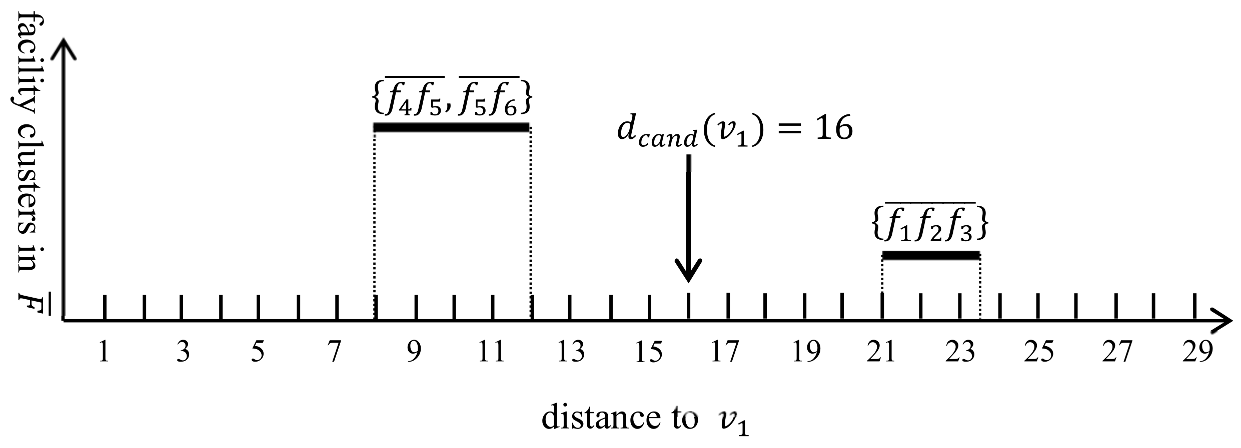
summarizes the computation of the candidate facilities at border points $v_1$ and $v_2$ of the query segment $\overline{v_1{v}_2}$ and includes the largest distances between the border points and the facility clusters in $\overline{F}$, candidate distances, and sets of candidate facilities at the border points. Recall that the kFN queries are issued only at the border points of the query segment, in which the query point q stays to find the candidate facilities for the query segment. Thus, for the example MkFN query, MOFA evaluates the kFN queries at border points $v_1$ and $v_2$ to find the candidate facilities for $\overline{v_1{v}_2}$. First, the kFN query is evaluated at $v_1$. The largest distances between $v_1$ and the facility clusters in $\overline{F}$ are calculated. Subsequently, the facility clusters $\overline{F_C}$ are arranged in a descending order based on $d_{max}(v_1,\overline{F_C})$. Figure 10 depicts that the facility clusters $\left\{\overline{f_1{f}_2{f}_3}\right\}$ and $\{\overline{f_4{f}_5},\overline{f_5{f}_6}\}$ are sorted using their largest distance to $v_1$ as follows: $\overline{F}=\{\left\{\overline{f_1{f}_2{f}_3}\right\},\{\overline{f_4{f}_5},\overline{f_5{f}_6}\}\}$. $\left\{\overline{f_1{f}_2{f}_3}\right\}$ is investigated, followed by $\{\overline{f_4{f}_5},\overline{f_5{f}_6}\}$. After exploring $\left\{\overline{f_1{f}_2{f}_3}\right\}$, $v_1$ chooses $f_1$, $f_2$, and $f_3$ as the candidate facilities for $\overline{v_1{v}_2}$ because the distance from $v_1$ to the second FN ($f_1$ or $f_3$) is 21, and the candidate distance for $v_1$ is $d_{cand}\left(v_1\right)=16$. The distances from $v_1$ to $f_1$, $f_2$, and $f_3$ are $d(v_1,f_1)=21$, $d(v_1,f_2)=22$, and $d(v_1,f_3)=2$1, respectively (Figure 6). The other facility cluster $\{\overline{f_4{f}_5},\overline{f_5{f}_6}\}$ does not need be explored because $d_{cand}\left(v_1\right)=16$ is larger than $d_{max}(v_1,\{\overline{f_4{f}_5},\overline{f_5{f}_6}\})=12$ (Figure 10). Finally, a set of candidate facilities at $v_1$ is evaluated as $\mathrm{\Sigma }\left(v_1\right)=\{f_1,f_2,f_3\}$.

In the same manner, the kFN query is evaluated at $v_2$ to find the candidate facilities for the query segment $\overline{v_1{v}_2}$. The largest distances between $v_2$ and the facility clusters in $\overline{F}$ are calculated. The facility clusters $\overline{F_C}$ are then arranged in a descending order based on $d_{max}(v_2,\overline{F_C})$. Figure 11 shows that the facility clusters $\left\{\overline{f_1{f}_2{f}_3}\right\}$ and $\{\overline{f_4{f}_5},\overline{f_5{f}_6}\}$ are sorted using their largest distance to $v_2$ as follows: $\overline{F}=\{\left\{\overline{f_1{f}_2{f}_3}\right\},\{\overline{f_4{f}_5},\overline{f_5{f}_6}\}\}$. $\left\{\overline{f_1{f}_2{f}_3}\right\}$ is investigated, followed by $\{\overline{f_4{f}_5},\overline{f_5{f}_6}\}$. After exploring $\left\{\overline{f_1{f}_2{f}_3}\right\}$, $v_2$ chooses $f_1$, $f_2$, and $f_3$ as the candidate facilities for the query segment $\overline{v_1{v}_2}$ because the distance from $v_2$ to the second FN $f_1$ is 17, and the candidate distance for $v_2$ is $d_{cand}\left(v_2\right)=12$. The distances from $v_2$ to $f_1$, $f_2$, and $f_3$ are $d(v_2,f_1)=17$, $d(v_2,f_2)=18$, and $d(v_2,f_3)=16$, respectively (Figure 8). The other facility cluster $\{\overline{f_4{f}_5},\overline{f_5{f}_6}\}$ does not have to be explored because $d_{cand}\left(v_2\right)=12$ is larger than $d_{max}(v_2,\{\overline{f_4{f}_5},\overline{f_5{f}_6}\})=7$ (Figure 11). Finally, a set of candidate facilities at $v_2$ is evaluated as $\mathrm{\Sigma }\left(v_2\right)=\{f_1,f_2,f_3\}$.

6.2. Computing the Valid Segments for the Query Segment $\overline{v_1{v}_2}$

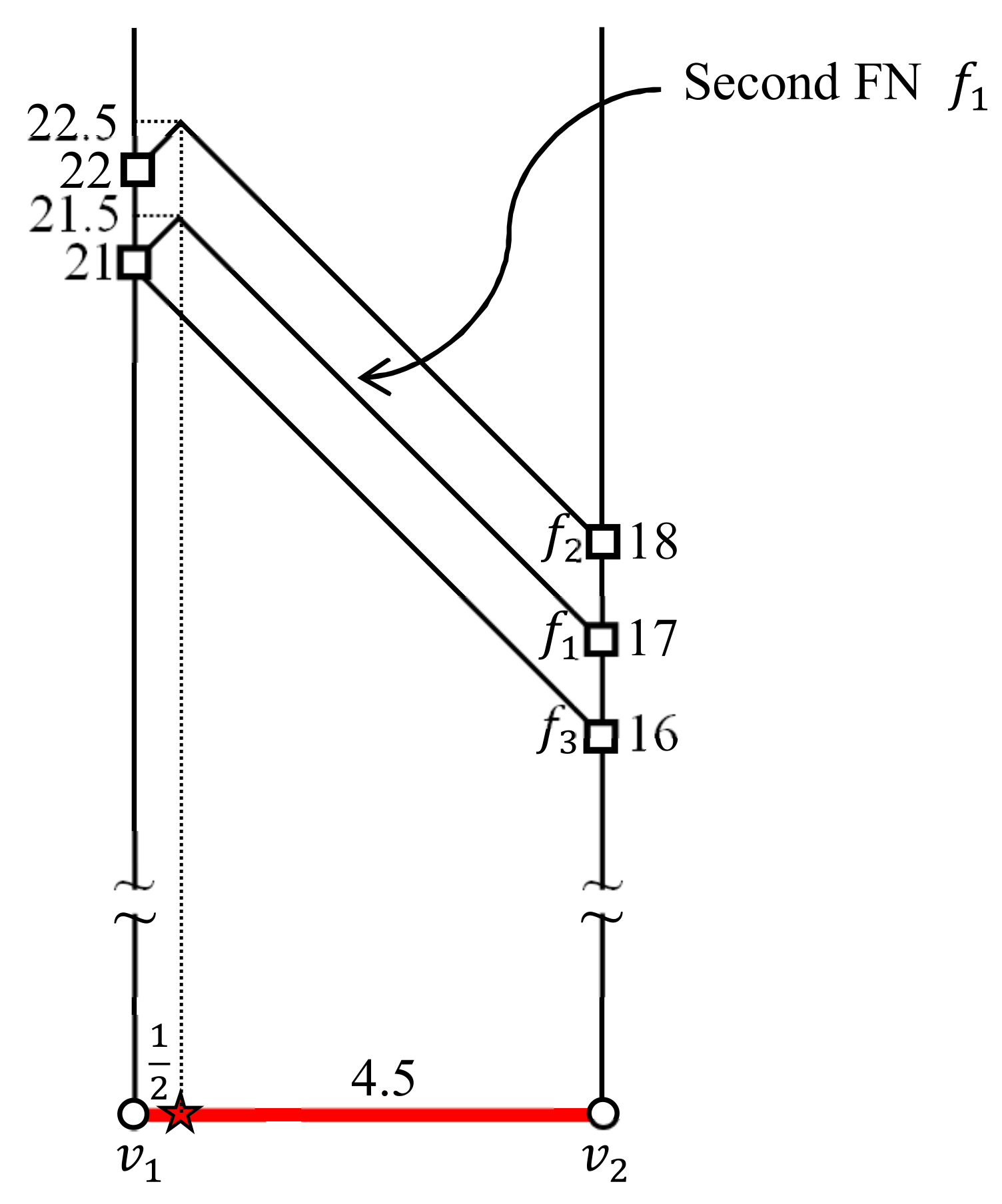
Figure 12 shows the changes in the distance from each candidate facility f to a query point q in $\overline{v_1{v}_2}$, where $f\in \{f_1,f_2,f_3\}$. The distance from $f_1$ to $v_1$ ($v_2$) is $d(f_1,v_1)=21$ ($d(f_1,v_2)=17$). Figure 12a demonstrates the change in the distance from $f_1$ to q in $\overline{v_1{v}_2}$. The shortest path from $f_1$ to q in $\overline{v_1{v}_2}$ is either $f_1\to v_1\to q$ or $f_1\to v_2\to q$. The distance from $f_1$ to q is evaluated as $d(f_1,q)=\left\{min(d(f_1,v_1)+len\left(\overline{v_{1}q}\right),d(f_1,v_2)+len\left(\overline{v_{2}q}\right))\right|q\in \overline{v_1{v}_2}\}$$=\left\{min(21+len\left(\overline{v_{1}q}\right),17+len\left(\overline{v_{2}q}\right))\right|q\in \overline{v_1{v}_2}\}$, where $len\left(\overline{v_{1}q}\right)+len\left(\overline{v_{2}q}\right)=5$. Similarly, the change in the distance from $f_2$ to q in $\overline{v_1{v}_2}$ can be drawn (Figure 12b), where $d(f_2,v_1)=22$ and $d(f_2,v_2)=18$. In the same manner, the change in the distance from $f_3$ to q in $\overline{v_1{v}_2}$ can also be drawn (Figure 12c), where $d(f_3,v_1)=21$ and $d(f_3,v_2)=16$.

Figure 13 plots $d(q,f_1)$, $d(q,f_2)$, and $d(q,f_3)$ together, which are illustrated in Figure 12a–c, respectively, to compute the valid segments in $\overline{v_1{v}_2}$. Recall that the query points in the valid segment have the same k FNs. The example MkFN query requires two facilities farthest from the query point q in $\overline{v_1{v}_2}$; hence, the second FN must be identified from each query point q. Figure 13 shows that facility $f_1$ is the second FN for the entire query segment $\overline{v_1{v}_2}$, and facility $f_2$ is farther from the query point q than the second FN $f_1$. Therefore, a valid segment can be found in $\overline{v_1{v}_2}$, and the query result is $\mathrm{\Phi }\left(\overline{v_1{v}_2}\right)=\left\{〈\overline{v_1{v}_2},\left\{f_1,f_2\right\}〉\right\}$.

7. Empirical Evaluation

Section 7.1 describes the empirical settings considered in this study. Section 7.2 presents the experimental results. In this section, we empirically evaluate the proposed MOFA and its conventional solution under various circumstances.

7.1. Empirical Settings

Table 3. Real road networks.

Road Network	Description	Vertices	Edges	Vertex lists
SJ	City streets in San Joaquin, California	18,263	23,874	20,040
NA	Highways in North America	175,813	179,179	12,416
SF	City streets in San Francisco, California	174,956	223,001	192,276

describes the three real-world road networks [28] considered in our empirical evaluation. These road networks are part of the road network in the United States and vary in size. Ten query points were considered to measure query execution time. The query points regularly evaluate kFN queries, and each query point moves within a query segment. A data space can typically be considered as a unit square with its upper-left corner at the coordinate (0,0) and its lower-right corner at (1,1). Facilities were generated to simulate highly skewed point of interest distributions. First, the centroids $c_1,c_2,\cdots ,c_m$ are randomly populated within the data space, where m$(1\le m\le 10)$ denotes the total number of centroids. The facilities around each centroid exhibit a Gaussian distribution with the mean indicating the centroid and the standard deviation set to ${\sigma =10}^{-2}$.

Table 4. Empirical settings.

Parameter	Range
Number of query points ($\left|Q\right|$)	10
Number of facilities ($\left|F\right|$)	1, 2, 3, 4, 5 ($\times {10}^3$)
Number of FNs required (k)	1, 2, 4, 8, 16
Query frequency in the query segment ($Q_F$)	2, 4, 8, 10, 20
Distribution of facilities	Gaussian distribution
Number of centroids for the facilities in F ($\left|C\right|$)	1, 3, 5, 7, 10
Standard deviation for the normal distribution ($\sigma$)	${10}^{-2}$
Road network	SJ, NA, SF

lists the empirical parameter settings. Each of these parameters was determined through a series of experiments in which a single parameter was varied while the other parameters remained constant at the bolded default values.

A conventional algorithm regularly evaluates kFN queries for the moving query point q. This method was considered as a benchmark to evaluate MOFA’s performance. All algorithms were implemented using C++ in the Microsoft Visual Studio development environment. All common subroutines of the algorithms were reused for similar tasks. For this empirical study, it was assumed that all indexing structures of the algorithms were stored in the main memory to rapidly process the MkFN queries. This assumption has often been used in other studies [22,29] on online LBSs. Repeated evaluations were performed to compute the average time required to answer MkFN queries. The TNR method [30] was employed to quickly calculate the network distance between two points during query processing. The empirical study was executed on a computer running the Windows 11 operating system equipped with an 8-core processor (i9-9900) running at 3.1 GHz with 32 GB of RAM.

7.2. Empirical Results

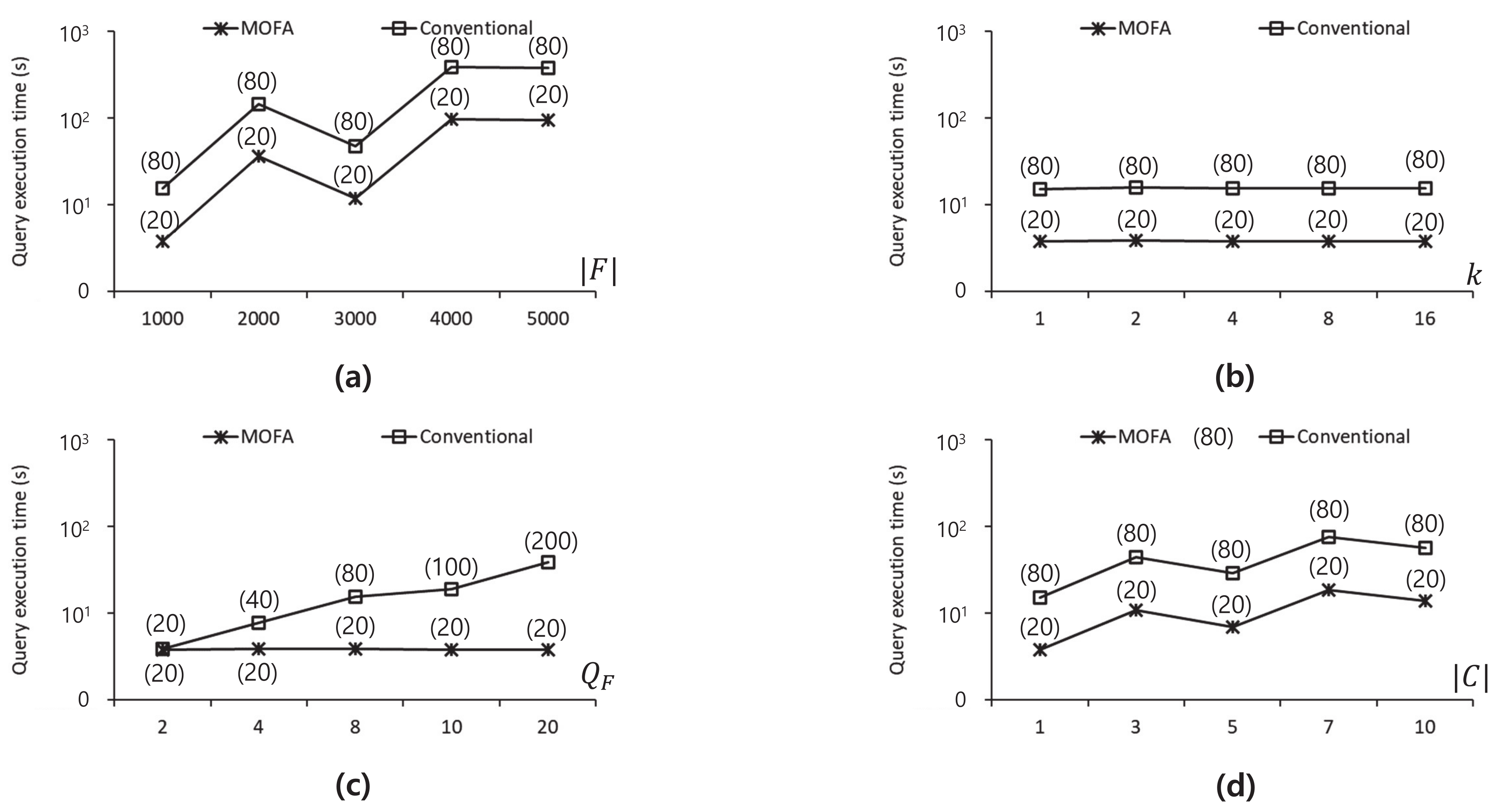
Figure 14 compares the proposed MOFA and conventional algorithm on the SJ road network. Each chart presents the MkFN execution time and number of kFN queries required to answer the MkFN query. The numbers in parentheses in Figure 14, Figure 15 and Figure 16 refer to the number of kFN queries required by MOFA and the conventional algorithm for answering the MkFN query. MOFA requires only two kFN queries to be evaluated to compute the valid segments for the query segment. However, the conventional algorithm requires kFN queries to be regularly evaluated to refresh the query results as the query point moves. In other words, the conventional algorithm evaluates a number of kFN queries linearly proportional to the query frequency, whereas MOFA evaluates only two kFN queries, regardless of the query frequency, as the query point moves within a query segment. Figure 14a presents the query execution times of MOFA and the conventional algorithm when the number of facilities varies from 1000 to 5000 (i.e., ${10}^3\le \left|F\right|\le 5\times {10}^3$). In all cases of $\left|F\right|$, MOFA outperforms the conventional algorithm. For this empirical study, 10 query points were considered with each query point evaluating eight kFN queries while moving along its query segment. Therefore, the MOFA and conventional algorithms evaluated 20 and 80 kFN queries, respectively. Figure 14b presents the query execution times when the number of FNs required varies from 1 to 16 (i.e., $1\le k\le 16$). For all cases of k, MOFA is approximately four times faster than the conventional algorithm. The query execution times of MOFA and the conventional algorithms are stable, regardless of k. This is because kFN query evaluation sorts facility clusters based on their distances to the query point and processes the sorted facility clusters. Figure 14c presents the query execution times when the query frequency varies from 2 to 20 (i.e., $2\le Q_F\le 20$). The query execution time of MOFA is stable and independent of the query frequency, whereas that of the conventional algorithm increases with the query frequency. Figure 14d presents the query execution times when the number of centroids for the facilities in F varies from 1 to 10 (i.e., $1\le \left|C\right|\le 10$). The kFN query execution time tends to increase with the $\left|C\right|$ value. This is because the facilities become more widely distributed as the $\left|C\right|$ value increases, resulting in an increase in query execution time.

Figure 15 compares the performance of MOFA and the conventional algorithm on the NA road network. The empirical results obtained using the NA road network exhibit performance patterns similar to those obtained using the SJ road network. Figure 15a presents the query execution times for ${10}^3\le \left|F\right|\le {5\times 10}^3$. MOFA is four times faster than the conventional algorithm. Figure 15b presents the query execution times for $1\le k\le 16$. Again, MOFA is four times faster than the conventional algorithm. The query execution times are stable and independent of the k value. Figure 15c presents the query execution times for $2\le Q_F\le 20$. MOFA is 1.0, 2.0, 4.2, 5.2, and 10.3 times faster than the conventional algorithm when $Q_F=2,4,8,10$, and 20, respectively. Figure 15d presents the query execution times for $1\le \left|C\right|\le 10$. MOFA is up to four times faster than the conventional algorithm.

Figure 16 presents the performance of MOFA and the conventional algorithm on the SF road network. Figure 16a presents the query execution times for ${10}^3\le \left|F\right|\le {5\times 10}^3$, indicating that MOFA outperforms the conventional algorithm by up to four times when $\left|F\right|=5000$. Figure 16b presents the query execution times for $1\le k\le 16$, indicating that MOFA outperforms the conventional algorithm by up to four times in terms of query execution time. The query execution times are stable and independent of the k value. Figure 16c presents the query execution times when $2\le Q_F\le 20$, indicating that MOFA is 1.0, 2.0, 4.2, 5.2, and 10.3 times faster than the conventional algorithm when $Q_F=2,4,8,10$, and 20, respectively. Figure 16d presents the query execution times for $1\le \left|C\right|\le 10$, indicating that MOFA is up to 4.2 times faster than the conventional algorithm when $\left|C\right|=10$. In summary, MOFA is faster than the conventional algorithm in all cases. In particular, the difference in performance between MOFA and the conventional algorithm increases with the query frequency. This confirms that MOFA benefits from the rapid retrieval of candidate facilities at the border points of the query segment and from the computation of valid segments for the query segment.

8. Conclusions

This study was motivated by the fact that moving query points such as pedestrians and vehicles, arbitrarily move within a road network. Therefore, existing solutions based on Euclidean distances cannot provide spatial queries for road network databases. This study proposed a moving farthest search algorithm called MOFA to compute valid segments for the query segment where a query point is located. MOFA performs an initial batch processing of MkFN queries in road networks to retrieve candidate facilities once and then computes the valid segments for the query segment. Empirical evaluation demonstrated that MOFA significantly outperformed the conventional algorithm and provided stable performance, regardless of the query frequency.

References

- Curtin, R.R.; Echauz, J.R.; Gardner, A.B. Exploiting the structure of furthest neighbor search for fast approximate results. Inf. Syst. 2019, 80, 124–135. [Google Scholar] [CrossRef]
- Gao, Y.; Shou, L.; Chen, K.; Chen, G. Aggregate farthest-neighbor queries over spatial data. In Proceedings of the International Conference on Database Systems for Advanced Applications, Hong Kong, China, 22–25 April 2011; pp. 149–163. [Google Scholar]
- Liu, J.; Chen, H.; Furuse, K.; Kitagawa, H. An efficient algorithm for arbitrary reverse furthest neighbor queries. In Proceedings of the Asia-Pacific Web Conference on Web Technologies and Applications, Kunming, China, 11–13 April 2012; pp. 60–72. [Google Scholar]
- Liu, W.; Yuan, Y. New ideas for FN/RFN queries based nearest Voronoi diagram. In Proceedings of the International Conference on Bio-Inspired Computing: Theories and Applications, Huangshan, China, 12–14 July 2013; pp. 917–927. [Google Scholar]
- Tran, Q.T.; Taniar, D.; Safar, M. Reverse k nearest neighbor and reverse farthest neighbor search on spatial networks. Trans. Large-Scale Data- Knowl.-Centered Syst. 2009, 1, 353–372. [Google Scholar]
- Wang, H.; Zheng, K.; Su, H.; Wang, J.; Sadiq, S.W.; Zhou, X. Efficient aggregate farthest neighbour query processing on road networks. In Proceedings of the Australasian Database Conference on Databases Theory and Applications, Brisbane, Australia, 14–16 July 2014; pp. 13–25. [Google Scholar]
- Xu, X.-J.; Bao, J.; Yao, B.; Zhou, J.; Tang, F.; Guo, M.; Xu, J. Reverse furthest neighbors query in road networks. J. Comput. Sci. Technol. 2017, 32, 155–167. [Google Scholar] [CrossRef]
- Yao, B.; Li, F.; Kumar, P. Reverse furthest neighbors in spatial databases. In Proceedings of the International Conference on Data Engineering, Shanghai, China, 29 March–2 April 2009; pp. 664–675. [Google Scholar]
- Liu, Y.; Gong, X.; Kong, D.; Hao, T.; Yan, X. A Voronoi-based group reverse k farthest neighbor query method in the obstacle space. IEEE Access 2020, 8, 50659–50673. [Google Scholar] [CrossRef]
- Huang, Q.; Feng, J.; Fang, Q.; Ng, W. Two efficient hashing schemes for high-dimensional furthest neighbor search. IEEE Trans. Knowl. Data Eng. 2017, 29, 2772–2785. [Google Scholar] [CrossRef]
- Liu, W.; Wang, H.; Zhang, Y.; Qin, L.; Zhang, W. I/O efficient algorithm for c-approximate furthest neighbor search in high dimensional space. In Proceedings of the International Conference on Database Systems for Advanced Applications, Jeju, Korea, 24–27 September 2020; pp. 221–236. [Google Scholar]
- Pagh, R.; Silvestri, F.; Sivertsen, J.; Skala, M. Approximate furthest neighbor in high dimensions. In Proceedings of the International Conference on Similarity Search and Applications, Glasgow, UK, 12–14 October 2015; pp. 3–14. [Google Scholar]
- Wang, S.; Cheema, M.A.; Lin, X.; Zhang, Y.; Liu, D. Efficiently computing reverse k furthest neighbors. In Proceedings of the International Conference on Data Engineering, Helsinki, Finland, 16–20 May 2016; pp. 1110–1121. [Google Scholar]
- Huang, Q.; Feng, J.; Fang, Q. Reverse query-aware locality-sensitive hashing for high-dimensional furthest neighbor search. In Proceedings of the International Conference on Data Engineering, San Diego, CA, USA, 19–22 April 2017; pp. 167–170. [Google Scholar]
- Aly, A.M.; Aref, W.G.; Ouzzani, M. Spatial queries with two kNN predicates. In Proceedings of the International Conference on Very Large Data Bases, Istanbul, Turkey, 27–31 August 2012; pp. 1100–1111. [Google Scholar]
- Gu, Y.; Yu, G.; Yu, X. An efficient method for k nearest neighbor searching in obstructed spatial databases. J. Inf. Sci. Eng. 2014, 30, 1569–1583. [Google Scholar]
- Nutanong, S.; Zhang, R.; Tanin, E.; Kulik, L. Analysis and evaluation of V*-kNN: An efficient algorithm for moving kNN queries. VLDB J. 2010, 19, 307–332. [Google Scholar] [CrossRef]
- Yung, D.; Yiu, M.L.; Lo, E. A safe-exit approach for efficient network-based moving range queries. Data Knowl. Eng. 2012, 72, 126–147. [Google Scholar] [CrossRef]
- Cho, H.-J. Batch processing algorithm for moving k-farthest neighbor queries in road networks. In Proceedings of the KSCI Summer Conference 2021, Jeju, Korea, 15–17 July 2021; pp. 223–224. [Google Scholar]
- Cho, H.-J. Cluster nested Loop k-farthest neighbor join algorithm for spatial networks. ISPRS Int. J. Geo-Inf. 2022, 11, 123. [Google Scholar] [CrossRef]
- Cho, H.-J.; Attique, M. Group processing of multiple k-farthest neighbor queries in road networks. IEEE Access 2020, 8, 110959–110973. [Google Scholar] [CrossRef]
- Abeywickrama, T.; Cheema, M.A.; Taniar, D. k-nearest neighbors on road networks: A journey in experimentation and in-memory implementation. In Proceedings of the International Conference on Very Large Data Bases, New Delhi, India, 5–9 September 2016; pp. 492–503. [Google Scholar]
- Lee, K.C.K.; Lee, W.-C.; Zheng, B.; Tian, Y. ROAD: A new spatial object search framework for road networks. IEEE Trans. Knowl. Data Eng. 2012, 24, 547–560. [Google Scholar] [CrossRef]
- Zhong, R.; Li, G.; Tan, K.-L.; Zhou, L.; Gong, Z. G-tree: An efficient and scalable index for spatial search on road networks. IEEE Trans. Knowl. Data Eng. 2015, 27, 2175–2189. [Google Scholar] [CrossRef]
- Zhang, M.; Li, L.; Hua, W.; Zhou, X. Efficient batch processing of shortest path queries in road networks. In Proceedings of the International Conference on Mobile Data Management, Hong Kong, China, 10–13 June 2019; pp. 100–105. [Google Scholar]
- Zhang, M.; Li, L.; Hua, W.; Zhou, X. Batch processing of shortest path queries in road networks. In Proceedings of the Australasian Database Conference on Databases Theory and Applications, Sydney, Australia, 29 January–1 February 2019; pp. 3–16. [Google Scholar]
- Zeng, W.; Church, R.L. Finding shortest paths on real road networks: The case for A*. Int. J. Geogr. Inf. Sci. 2009, 23, 531–543. [Google Scholar] [CrossRef]
- Real Datasets for Spatial Databases. Available online: https:/www.cs.utah.edu/~lifeifei/SpatialDataset.htm (accessed on 28 May 2022).
- Wu, L.; Xiao, X.; Deng, D.; Cong, G.; Zhu, A.D.; Zhou, S. Shortest path and distance queries on road networks: An experimental evaluation. In Proceedings of the International Conference on Very Large Data Bases, Istanbul, Turkey, 27–31 August 2012; pp. 406–417. [Google Scholar]
- Bast, H.; Funke, S.; Matijevic, D. Ultrafast shortest-path queries via transit nodes. In Proceedings of the International Workshop on Shortest Path Problem, Piscataway, NJ, USA, 13–14 November 2006; pp. 175–192. [Google Scholar]
Figure 1.
Example of MkFN queries in a road network.
Figure 2.
Interaction between the moving query point q and location-based service (LBS) server while q moves along .
Figure 3.
Example of an MkFN query q in a road network.
Figure 4.
Segmentation of an example road network using road intersections.
Figure 5.
Clustering method for grouping facilities into facility clusters: (a) grouping facilities into facility segments; (b) grouping facility segments into facility clusters.
Figure 6.
and .
Figure 7.
and ; (a) and ; (b) and .
Figure 8.
Figure 9.
Figure 10.
Arrangement of the facility clusters based on their largest distance to .
Figure 11.
Figure 12.
Changes in the distance from each candidate facility f to a query point q in : (a) change of for ; (b) change of for ; (c) change of for .
Figure 13.
Plot of , , and for .
Figure 14.
Performance comparisons between MOFA and the conventional algorithm on the SJ road network: (a) ; (b) ; (c) ; (d) .
Figure 15.
Performance comparisons between MOFA and the conventional algorithm on the NA road network: (a) ; (b) ; (c) ; (d) .
Figure 16.
Performance comparisons between MOFA and the conventional algorithm on the SF road network: (a) ; (b) ; (c) ; (d) .