Clustering Algorithm with a Greedy Agglomerative Heuristic and Special Distance Measures

Abstract

Automatic grouping (clustering) involves dividing a set of objects into subsets (groups) so that the objects from one subset are more similar to each other than to the objects from other subsets according to some criterion. Kohonen neural networks are a class of artificial neural networks, the main element of which is a layer of adaptive linear adders, operating on the principle of “winner takes all”. One of the advantages of Kohonen networks is their ability of online clustering. Greedy agglomerative procedures in clustering consistently improve the result in some neighborhood of a known solution, choosing as the next solution the option that provides the least increase in the objective function. Algorithms using the agglomerative greedy heuristics demonstrate precise and stable results for a k-means model. In our study, we propose a greedy agglomerative heuristic algorithm based on a Kohonen neural network with distance measure variations to cluster industrial products. Computational experiments demonstrate the comparative efficiency and accuracy of using the greedy agglomerative heuristic in the problem of grouping of industrial products into homogeneous production batches.

1. Introduction

The search for a clustering algorithm that has both high accuracy and stability of the result, and, at the same time, a high speed of operation, is one of the problems of cluster analysis. The clustering result depends on the initially selected number of subsets, as well as the selected measure of similarity (dissimilarity) [1]. One of the most famous automatic grouping models is the k-means model [2], which was proposed by Steinhaus [3]. The goal of the k-means problem is to find k points (centers, centroids) X₁, …, X_k in an M-dimensional space, such that the sum of the squared distances from the known points (data vectors) A₁, …, A_m to the nearest of the required points reaches a minimum:

$$\arg \min F(X_1,\dots ,X_k)={\displaystyle \sum _{j\in \{1,k\}}\min {\Vert X_j-A_i\Vert }^2}.$$

(1)

Optimization model (1) can be considered as a location problem, where the points X_j have to be placed in an optimal way. Location theory has been developing for a long time separately from cluster analysis while solving very close or completely identical problems. Weiszfeld proposed an iterative procedure for solving the Weber problem, one of the simplest location problems, based on an iterative weighted least squares method [4]. This algorithm determines a set of weights that are inversely proportional to the distances from the current estimate to the sample points and creates a new estimate that is the weighted average of the sample according to these weights. In specific situations, Weiszfeld’s algorithm is very slow and does not always converge.

Local search methods for solving location problems are used in Ref. [5]. The standard local descent algorithm starts with an initial solution S = {X₁, …, X_k}, chosen randomly or with the help of some auxiliary algorithm. At each step of the local descent, there is a transition from the current solution to a neighboring solution with a smaller value of the objective function until the local optimum is reached. The key problem here is to find the set of neighboring solutions n(S). At each step of the local search, the neighborhood function n(S) specifies a set of possible search directions. Neighborhood functions can be very diverse, and the neighborhood relation is not always symmetrical. Local search algorithms are widely used to solve NP-hard discrete optimization problems. However, simple local descent does not allow the finding of the global optimum of the problem.

Local search methods were further developed in so-called metaheuristics, in particular in the search algorithm with variable neighborhoods (variable neighborhoods search, VNS). Its main idea is to systematically change the neighborhood function and the corresponding change in the landscape during the local search.

The k-means problem was algorithmically implemented by S. Lloyd [6]. For the observation vector X, the k-means algorithm is designed to determine k centers and assign data points (objects) to each center to form clusters C_j, j = 1… k while minimizing the difference between the objects within the cluster. In the k-means algorithm, it is necessary to initially predict the number of groups (clusters).

In addition, the result obtained depends on the initial choice of centers, which is one of the main disadvantages of the algorithm. The modern literature offers many approaches to setting the initial centroids for the k-means algorithm, which are basically various evolutionary and random search methods. One of the most popular methods is the k-means++ algorithm [7], where the first centroid is chosen randomly and further selection goes with a certain probability. Moreover, in Ref. [8], a similar method is developed based on finding areas with maximum density. In Ref. [9], the authors propose a brute-force approach to the initialization of the k-means algorithm. Kalczynski et al. in Ref. [10] introduce three algorithms (merging, construction and separation) to create starting solutions of the k-means problem. In Ref. [11], a heuristic-based algorithm to improve the initial seeding of the k-means clustering described is implemented, where a hybrid approach with a genetic algorithm and the differential evolution heuristic is used. Detailed overviews of the existing initialization approaches may be found in Refs. [12,13,14].

The Kohonen neural network [15] of the vector quantization type is an autoassociator closely related to k-means. This competitive network can be related to unsupervised learning. The Kohonen learning law is an algorithm that finds the centroid (called “codebook vector”) closest to each training case and moves the winning centroid closer to the training case. Another type of Kohonen network is the self-organizing map competitive network that provides a topological mapping from the input space to the clusters. Kohonen networks are used in many fields of interest, such as speech recognition [16,17], image compression [18,19], image segmentation [20], face recognition [21,22,23], classification of weather patterns [24], malware detection [25], seasonal sales planning [26], medical decision-making [27,28], e-learning recommendations [29], denial of service attack defense detection [30], groundwater quality assessment [31], exploration of the investment patterns [32] and others.

Greedy agglomerative heuristic procedures [33,34] are tools to improve a result in a certain neighborhood of the solution. An agglomerative procedure starts with some solution S containing an excessive number of centroids and sequentially removes them. The elements of the clusters, related to the removed centroids, are redistributed among the remaining clusters. The greedy strategies are used to decide which clusters are most similar to be merged together at each iteration of the agglomerative procedure. For subsequent iterations, the chosen method is that which gave the best increase in the objective function in the previous iterations. The practice of solving NP-hard problems shows the efficiency of the transition from randomized recombination procedures to the search for the best recombination method [35]. The authors in Ref. [36] proposed methods of greedy agglomerative heuristics based on the location theory models. Algorithms using these methods are often randomized, but the results are quite stable. The method of greedy agglomerative heuristics uses evolutionary algorithms as one of the ways to organize a global search.

To date, the vast majority of the algorithms developed for continuous location problems use the most common distance measures (Euclidean, Manhattan). However, taking into account the characteristics of the feature space of a specific practical problem, the choice of a distance measure can lead to an increase in the accuracy of clustering. For instance, Itakura–Saito distance was used to build the learning vector quantization algorithm. In Ref. [19], a method is proposed for using the Mahalanobis distance as the basis for grouping. The Mahalanobis distance was also used to cluster incoming data into neural nodes in a self-organizing incremental neural network [22]. Kohonen networks with graph-based augmented metrics are presented in Ref. [37]. In Ref. [38], a distance measure for a self-organizing map is defined based on data distribution, and it is calculated with the use of an energy function. A distance metric learning method is often applied. For instance, in Ref. [22], the Mahalanobis matrix is computed, which assures small distances between the nearest neighbor points from the same class and the separation of points belonging to different classes by a large margin. Metric learning for the SOM based on the adaptive subspaces is represented in Ref. [39]. Furukawa [40] offers a nonlinear metrics learning method. The authors in Ref. [41] use an ensemble approach to metric learning with objective function generalization. Yoneda and Furukawa [42] propose a co-training approach, which collapses the objective function, thereby avoiding undesirable local optima.

In our work, our aim is solving the problem of the automatic grouping of objects. As a base, we use different types of Kohonen networks and modify them with the greedy agglomerative heuristic and different types of distance measures. Then, we test our approach on the applied problem.

The rest of this paper is organized as follows. In the Section 2, we introduce the Kohonen neural network model and propose our new algorithm involving the greedy agglomerative heuristic procedure. In the Section 3, we describe the computational experiments with a practically important dataset. In the Section 4 and Section 5, we discuss the results and provide a short conclusion.

2. Kohonen Neural Networks for Clustering Problem

2.1. Distance Measures

In clustering problems, the key concept is the concept of distance metrics between objects. Metric is a function that determines the measure of the distance between objects in the metric space R_p. Metric space is a set of points with a distance function d(x_i, y_i). The distance of order p between two points is determined by the Minkowski function (l_p–norm) [1,43,44]:

$$d(x,y)={\left({\displaystyle \sum _{i=1}^M{\left|x_i-y_i\right|}^p}\right)}^{\frac{1}{p}},$$

(2)

where x and y are vectors of parameter values, M is the vector dimension. The parameter p is determined by the researcher; it can be used to progressively increase or decrease the weight of the i-th variable. Special cases of the Minkowski function depend on the p value. For p = 2, the function calculates the Euclidean distance between two points (l₂–norm):

$$d(x,y)=\sqrt{{\displaystyle \sum _{i=1}^M{\left(x_i-y_i\right)}^2}}.$$

(3)

The squared Euclidean distance is often used:

$$d(x,y)={\displaystyle \sum _{i=1}^M{\left(x_i-y_i\right)}^2}.$$

(4)

For p = 1, the function calculates the Manhattan distance, also called rectangular (l₁–norm):

$$d(x,y)={\displaystyle \sum _{i=1}^M\left|x_i-y_i\right|}.$$

(5)

For p = ∞, the function calculates the Chebyshev distance, returning the largest value of the difference between the object parameters modulo:

$$d(x,y)=\max \left|x_i-y_i\right|.$$

(6)

In addition to the cases of the dependence of the distance function on the parameter p, there are other methods for calculating distances, for example, the Mahalanobis distance [45]. Mahalanobis distance can be defined as a measure of dissimilarity (difference) between vectors from the same probability distribution with the covariance matrix C:

$$d(x,y)=\sqrt{{\displaystyle \sum _{i=1}^M{\left(x_i-y_i\right)}^T·C^{-1}·\left(x_i-y_i\right)}}.$$

(7)

If the covariance matrix is identity, then the distance becomes equal to Euclidean. The covariance matrix is defined as:

$$C=\mathrm{cov}(x,y)=\mu \left[\left(x-\mu (x)\right)\left(y-\mu (y)\right)\right],$$

(8)

where μ is expected value. In most cases, the literature presents problems with Euclidean or Manhattan metrics.

In our study, we use five different types of distance measures to evaluate which one is preferable in our case.

2.2. Vector Quantization Networks and Self-Organizing Kohonen Maps

A Kohonen network [15,39] is a self-organized neural network that enables us to allocate groups (clusters) of input vectors that have some common features. The Kohonen network (or Kohonen layer) is a single-layer network, each neuron of which is connected to all components of the input vector. The input vector is a description of one of the objects to be clustered. The number of neurons coincides with the number of clusters K that the network should allocate. Linear weighted adders are used as neurons in the Kohonen network. Each j-th neuron is described by a vector of weights W_j = (w_1j, w_2j, …, w_Mj), where M is input vector dimension, j = 1…K. The input vector has the form X_i = (x_1i, x_2i, …, x_Mi), i = 1…N, where N is number of objects.

According to the methods of adjusting the input weights of the adders and the problems being solved, many varieties of Kohonen networks are distinguished [46]. The most famous of them are:

• Vector quantization networks (VQ), closely related to k-means method;
• Self-organizing Kohonen maps (SOM), which provide a “topological” mapping from the input space to the clusters. Neurons in SOMs are organized into a grid (usually two-dimensional);
• Learning vector quantization networks (LVQ), which include supervised learning and used for classification problems.

First two types of Kohonen networks refer to unsupervised learning, considered in this article.

Vector quantization consists of replacing a continuous distribution by a finite set of quantizers while minimizing a predefined distortion criterion and may be used to determine groups (clusters) of data sharing common properties [46]. Since vector quantization is a natural application for k-means, the centroids are also referred to as a “codes”, and the table mapping codes to centroid is often referred to as a “codebook”.

Competition mechanisms are used to train the network according to principle “winner takes all”, for instance, simple competitive learning (SCL) algorithm [47]. When the vector X is fed to the network input, the neuron wins, the weight vector of which is the least different from the input vector: $d\left(X,W_{cl}\right)=\underset{1\le j\le K}{\min }d\left(X,W_j\right)$. This problem with K key vectors W_j in the feature space of the observed data X in terms of vector quantization is defined as a minimization of encoding distortion, i.e., as minimization problem:

$$D={\sum }_{j=1}^K{\sum }_{x\in V\left(j\right)}\left|\right|x-W_j\left|\right|{}^2 \to min$$

(9)

where V(j) consists of points X_i ∈ X closest to W_j.

The SCL algorithm is in fact the online version of the Lloyd’s algorithm. If all data points are known in advance, this algorithm works offline as a batch algorithm (batch vector quantization, BVQ). The k-means method is an intermediate version, where only one data point is randomly chosen, and only the winning centroid is updated as the mean value of its cluster [46]. Thus, we can say that Kohonen networks have an advantage over the k-means model in that they allow organizing the online clustering. Basic version of SCL algorithm is represented in Algorithm 1.

Algorithm 1. Basic SCL algorithm

Required: Set of initial data vectors X1, …, XN, where N is the number of points; set the number of neurons K; η0 (η = η0), where η0 is the initial learning rate; set the step of changing the learning rate Δη;

1. Set the weight of each neuron Wj ($j=1,K$)

2. While η > 0:

3. for $i=\overline{1,N}$ do

4. for $j=\overline{1,K}$ do

5. Find the closest neuron Wcl to Xi: $cl=arg\underset{1\le j\le K}{min}d\left(X_i,W_j\right)$

6. Update the closest neuron: Wcl = Wcl + η⋅(Xi − Wcl)

7. η = η − Δη

Self-organizing Kohonen maps [15,39] produce a mapping from a multidimensional input space onto a lattice of neurons. The mapping is topology-preserving in that neighboring neurons respond to “similar” input patterns. SOMs are typically organized as one- or two- dimensional lattices for the purpose of visualization and dimensionality reduction. During training, the winner neuron and its topological neighbors are adapted to make their weight vectors more similar to the input pattern that caused the activation. SOM algorithm with time limit is represented in Algorithm 2.

Thus, the SCL algorithm is a particular case of the SOM algorithm, when the neighborhood is reduced to zero. The magnitude of the changes decreases with time and is smaller for neurons far away from the winning neuron. The learning rates and neighborhood functions can be applied in various ways. However, these functions should be decreasing [48].

Algorithm 2. Basic SOM algorithm

Required: Set of initial data X1, …, XN, where N is the number of points; set the number of neurons K; η0 (η = η0), where η0 is the initial learning rate.

1. Set the weight of each neuron Wj ($j=1,K$)

2. t = 0

3. While maximum time is not exceeded: t ≤ Tmax:

4. Randomly choose Xi from initial data X1, …, XN.

5. Find the closest neuron Wcl to Xi: $cl=arg\underset{1\le j\le K}{min}d\left(X_i,W_j\right)$

6. Update the closest neuron Wcl and its neighbors V(Wcl).

Here, V(Wcl) is the set of indexes in the neighborhood of Wcl, including Wcl:

For each p in V(Wcl):

Wp = Wp + η(t) · h(t,d (Wp,Wcl)) · (Xi − Wp),

where η(t) is learning rate, h(t,d (Wp,Wcl)) is neighborhood function.

7. t = t + 1

8. End while

Several methods can be used to initialize the neurons. The simplest one is when the initial values are chosen randomly. Another method is to initialize the weights by the average of the minimum and the maximum values of the elements of the vectors that have to be classified.

Moreover, there are different types of stopping rules that can be applied at step 2 of Algorithm 1 and step 3 of Algorithm 2. A fixed threshold for the error, time limit of fixed number of algorithm repeating can be used.

2.3. Proposed Algorithms

For our purposes, we take as a basis the Kohonen network. First, we use vector quantization type (Algorithm 3). The idea is to initialize the excess number of neurons and then gradually decrease their number. The algorithm processes data points one by one. After a certain step, the neuron is removed, the removal of which shows the smallest increase in the value of the objective function. The learning rate decreases after a certain number of steps SN.

Algorithm 3. SCL-based algorithm with a greedy agglomerative heuristic (SCL-GREEDY)

Required: Set of initial data X1, …, XN, where N is the number of points; set the number of neurons K1; η0 (η = η0), where η0 is the initial learning rate; set the step of changing the learning rate Δη

1.  Increase the number of neurons k times K = K · K1

2.  Set the weight of each neuron Wj ($j=1,K$)

3.  Determine the number of steps to calculate η: SN = trunc(N/K), jj = 1

4.  While η > 0:

5.  For $i=\overline{1,N}$, do

6.  For $j=\overline{1,K}$, do

7.  Find the closest neuron Wcl to Xi: $cl=arg\underset{1\le j\le K}{min}d\left(X_i,W_j\right)$

8.  Update the closest neuron Wcl: Wcl = Wcl +η·(Xi − Wcl)

9.  For each neuron Wj, calculate sum of distances to the initial data

X1, …, Xi:

$S_j={\displaystyle \sum _{j=1}^K{\displaystyle \sum _{q=1}^i{\Vert W_j-X_q\Vert }^2}}$

10. IF i%(SN + 1) == 0, THEN Recalculate η: jj = jj + 1, η = η0/jj

11. IF K <> K1, THEN remove neuron Wj with the maximum sum of distances $S_j$

12. η = η – Δη

13. End while

SOM-based algorithm with a greedy agglomerative heuristic is represented in Algorithm 4.

Batch versions of described algorithms are similar to their online versions except that the neuron weights are recalculated after passing through all sample points. We denote batch version of SCL algorithm as BVQ (as in Ref. [46]) and batch version of SOM algorithm as BSOM.

Algorithm 4. SOM-based algorithm with a greedy agglomerative heuristic (SOM-GREEDY)

Required: Set of initial data X1, …, XN, where N is the number of points; set the number of neurons K1; η0 (η = η0), where η0 is the initial learning rate.

1. Increase the number of neurons k times K = k · K1

2. Set the weight of each neuron Wj ($j=1,K$)

3. t = 0

4. While maximum time is not exceeded: t ≤ Tmax:

5. Randomly choose Xi from initial data X1, …, XN.

6. Find the closest neuron Wcl to Xi: $cl=arg\underset{1\le j\le K}{min}d\left(X_i,W_j\right)$

7. Update the closest neuron Wcl and its neighbors V(Wcl).

Here, V(Wcl) is the set of indexes in the neighborhood of Wcl, including Wcl:

For each p in V(Wcl):

Wp = Wp + η(t) · h(t,d (Wp,Wcl)) · (Xi − Wp),

where η(t) is learning rate, h(t,d (Wp,Wcl)) is neighborhood function.

8. For each neuron Wj, calculate sum of distances to the initial data X1, …, Xi: $S_j={\displaystyle \sum _{j=1}^K{\displaystyle \sum _{q=1}^i{\Vert W_j-X_q\Vert }^2}}$

9. IF K <> K1, THEN remove neuron Wj with the maximum sum of distances $S_j$

10. η = η − Δη

11. t = t + 1

12. End while

3. Computational Experiment and Analysis

For the experiment, we considered the sample consisting of four different homogeneous batches of electronic radio components [49]. The total number of devices in all batches is 446. We considered various combinations of batches: mixed lots from four, three and two batches. Four-batch mixed lot contains 62 parameters (features), three-batch mixed lot and two-batch mixed lot contain 41 parameters. The difficulty of the sample is that the number of parameters in it is large enough relative to the number of sample elements.

Each experiment is performed in online mode and in batch mode. We used different types of distance measures: Chebyshev distance (ChD), Euclidean distance (EuD), squared Euclidean distance (SEuD), Mahalanobis distance (MahD), Manhattan distance (ManD). The choice of the method for initializing the weight coefficients was also different: average, random and with preliminary clustering by the k-means algorithm. Each experiment was run 30 times.

Algorithms were implemented in Java. For the computational experiments, we used the following test system: AMD Ryzen 5-1600 6C/12T 3200MHz CPU, 16 CB RAM. Each experiment took an average of 1 min of computer time.

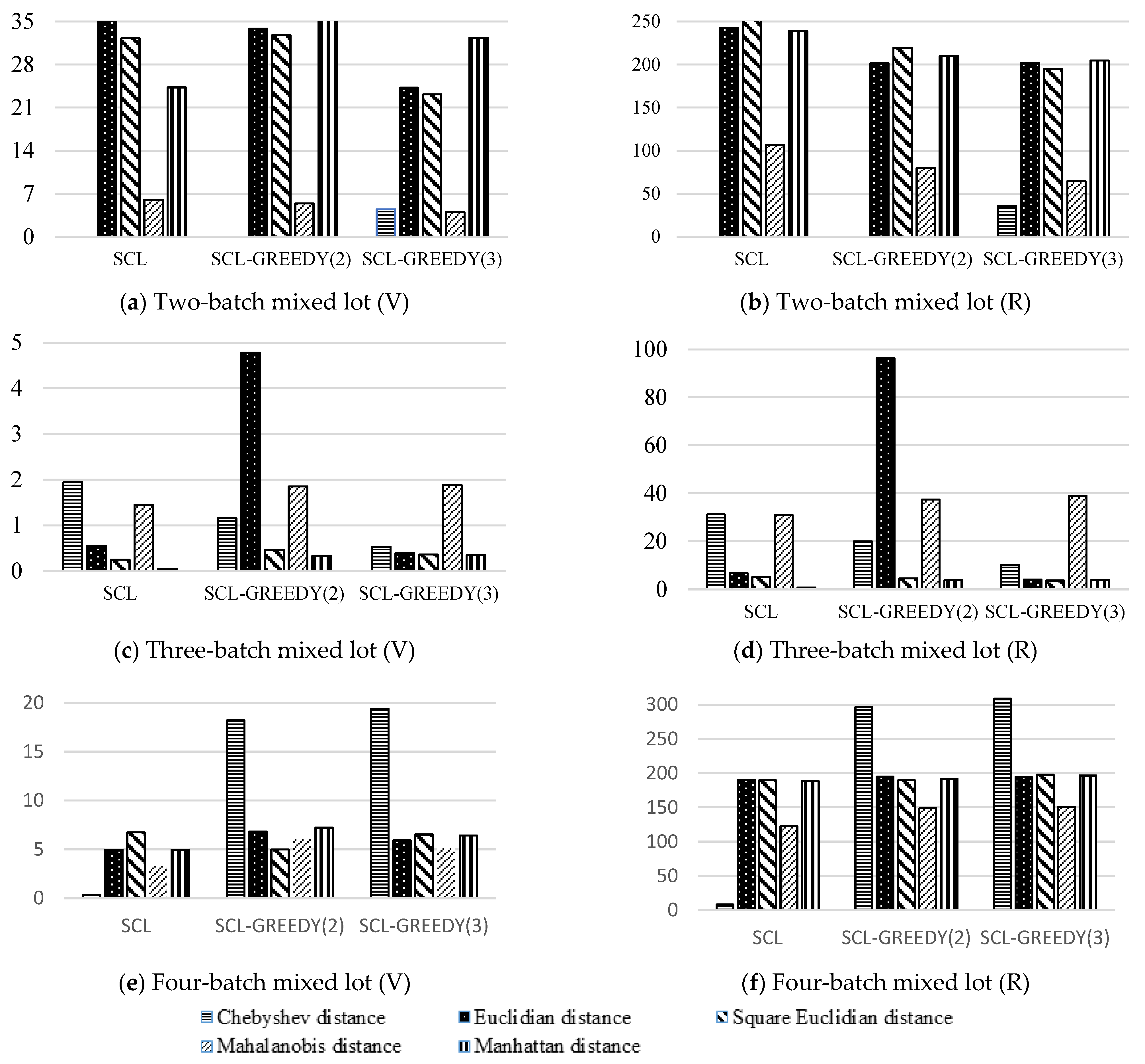
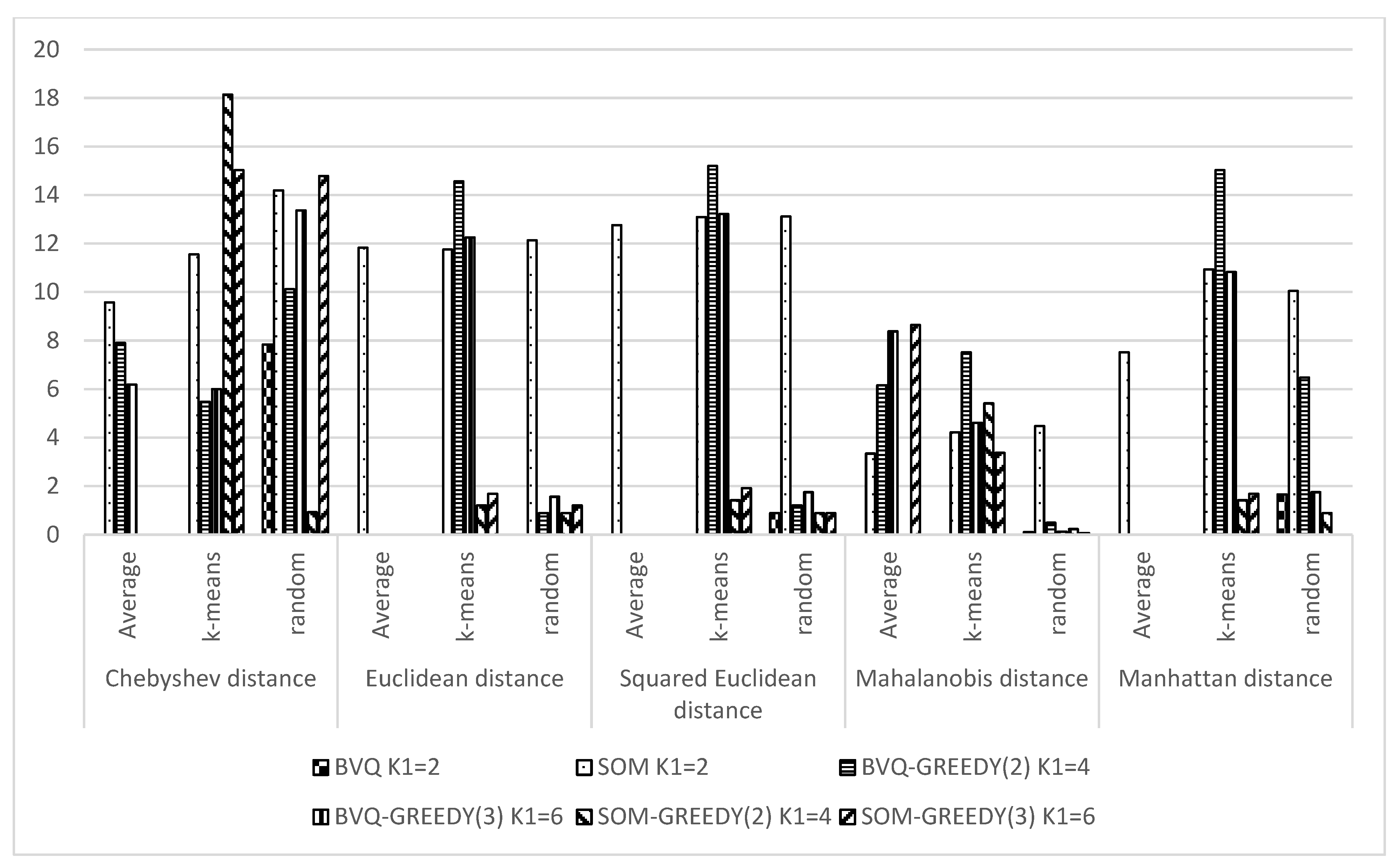
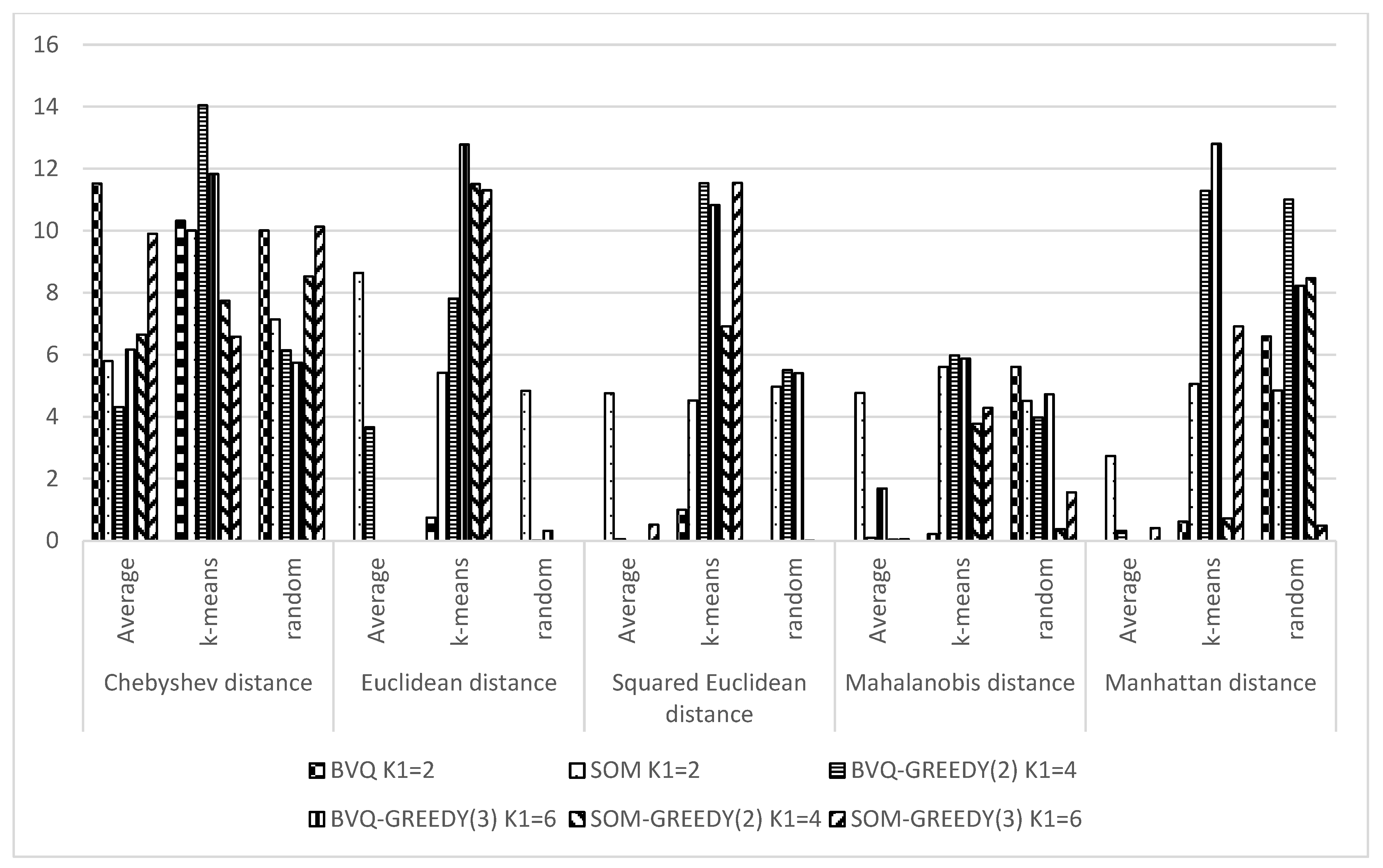
3.1. Experiments in Online Mode

In this section, we compare the results of the experiment performed with SCL and SCL-GREEDY methods. Experiment with initial number of neurons K1 coinciding with a given number of clusters is marked as SCL; experiments with the initial number of neurons exceeding the specified number of clusters by two (K = 2 × K1) and three (K = 3 × K1) times are marked as SCL-GREEDY(2) and SCL-GREEDY(3).

Computational experiments showed that the use of the greedy agglomerative heuristic in SCL algorithm, in most cases, improves the accuracy of batch separation. Moreover, clustering accuracy decreases with increasing number of homogeneous batches in a mixed lot (Figure 1).

With regard to the influence of the distance measure on the clustering accuracy, it can be noted that the Chebyshev distance has an advantage over the others except two-batch mixed lot. However, in the case of the Chebyshev distance, we were dealing with a large coefficient of variation and a span coefficient for 3 and 4 mixed lots.

Moreover, for various combinations of batches, the minimum (Min), maximum (Max), mean (Mean), standard deviation (σ), coefficient of variation (V) and the span factor (R) of the objective function are calculated (

Table 1. Objective function value summarized after 30 attempts (Chebyshev distance).

Parameter	SCL	SCL-GREEDY(2)	SCL-GREEDY(3)
Two-batch mixed lot (p < 0.00001)
	K1 = 2	K1 = 4	K1 = 6
Min	415.627	371.1297	301.2941
Max	415.627	371.1322	337.3007
Mean	415.627	371.1301	329.2811 1
σ	6.38E-12	0.000772	14.67288
V	1.53E-12	0.000208	4.456033
R	2.80E-11	0.002558	36.00667
Three-batch mixed lot (p < 0.00001)
	K1 = 3	K1 = 6	K1 = 9
Min	406.912	397.815	397.787
Max	438.101	417.747	407.933
Mean	431.002	415.140	406.966
σ	8.395	4.783	2.167
V	1.948	1.152	0.533
R	31.189	19.933	10.146
Four-batch mixed lot (p = 0.61708)
	K1 = 4	K1 = 8	K1 = 12
Min	606.056	596.008	594.863
Max	614.033	892.644	903.672
Mean	609.644	689.886	704.368
σ	2.167	125.611	136.492
V	0.355	18.208	19.378
R	7.977	296.636	308.810

¹ The best mean values of objective function are given in bold if the difference between SCL algorithm and its greedy version is statistically significant at p ≤ 0.05 (statistical significance was tested using the Wilcoxon rank sum test).

,

Table 2. Objective function value summarized after 30 attempts (Euclidean distance).

Parameter	SCL	SCL-GREEDY(2)	SCL-GREEDY(3)
Two-batch mixed lot (p < 0.00001)
	K1 = 2	K1 = 4	K1 = 6
Min	198.486	193.825	191.610
Max	441.215	395.174	393.348
Mean	296.329	251.285	206.390 1
σ	104.214	84.992	50.003
V	35.168	33.823	24.228
R	198.486	193.825	191.610
Three-batch mixed lot (p = 0.00214)
	K1 = 3	K1 = 6	K1 = 9
Min	365.927	274.081	365.719
Max	372.730	370.565	369.705
Mean	371.892	366.467	367.961
σ	2.059	17.518	1.459
V	0.554	4.780	0.396
R	6.803	96.484	3.986
Four-batch mixed lot (p = 0.0012)
	K1 = 4	K1 = 8	K1 = 12
Min	952.563	939.212	914.629
Max	1142.812	1133.992	1108.637
Mean	1113.352	1084.122	1071.603
σ	55.095	74.012	63.228
V	4.949	6.827	5.900
R	952.563	939.212	914.629

¹ The best mean values of objective function are given in bold if the difference between SCL algorithm and its greedy version is statistically significant at p ≤ 0.05 (statistical significance was tested using the Wilcoxon rank sum test).

,

Table 3. Objective function value summarized after 30 attempts (squared Euclidean distance).

Parameter	SCL	SCL-GREEDY(2)	SCL-GREEDY(3)
Two-batch mixed lot (p < 0.00001)
	K1 = 2	K1 = 4	K1 = 6
Min	198.486	193.825	191.611
Max	450.382	413.390	386.087
Mean	312.271	228.919	205.969 1
σ	100.749	74.987	47.677
V	32.263	32.757	23.148
R	251.896	219.564	194.475
Three-batch mixed lot (p < 0.00001)
	K1 = 3	K1 = 6	K1 = 9
Min	367.557	366.012	366.085
Max	372.730	370.568	369.725
Mean	372.527	369.305	368.306
σ	0.942	1.715	1.324
V	0.253	0.464	0.360
R	5.173	4.556	3.640
Four-batch mixed lot (p = 0.02088)
	K1 = 4	K1 = 8	K1 = 12
Min	952.513	939.456	914.668
Max	1142.098	1129.014	1112.335
Mean	1097.790	1099.933	1067.170
σ	73.902	54.806	69.570
V	6.732	4.983	6.519
R	189.584	189.558	197.668

¹ The best mean values of objective function are given in bold if the difference between SCL algorithm and its greedy version is statistically significant at p ≤ 0.05 (statistical significance was tested using the Wilcoxon rank sum test).

,

Table 4. Objective function value summarized after 30 attempts (Mahalanobis distance).

Parameter	SCL	SCL-GREEDY(2)	SCL-GREEDY(3)
Two-batch mixed lot (p = 0.06288)
	K1 = 2	K1 = 4	K1 = 6
Min	352.603	359.915	356.673
Max	458.955	439.944	421.191
Mean	399.825	396.924	388.449
σ	24.151	21.471	15.522
V	6.040	5.409	3.996
R	106.353	80.029	64.519
Three-batch mixed lot (p = 0.00338)
	K1 = 3	K1 = 6	K1 = 9
Min	462.220	455.998	451.949
Max	493.155	493.356	490.924
Mean	484.589	480.276	476.854 1
σ	7.020	8.892	8.978
V	1.449	1.851	1.883
R	30.935	37.358	38.976
Four-batch mixed lot (p = 0.00034)
	K1 = 4	K1 = 8	K1 = 12
Min	962.070	980.266	959.326
Max	1084.960	1129.044	1109.918
Mean	1050.083	1044.941	996.063
σ	34.760	63.595	51.328
V	3.310	6.086	5.153
R	122.890	148.778	150.592

¹ The best mean values of objective function are given in bold if the difference between SCL algorithm and its greedy version is statistically significant at p ≤ 0.05 (statistical significance was tested using the Wilcoxon rank sum test).

and

Table 5. Objective function value summarized after 30 attempts (Manhattan distance).

Parameter	SCL	SCL-GREEDY(2)	SCL-GREEDY(3)
Two-batch mixed lot (p < 0.00001)
	K1 = 2	K1 = 4	K1 = 6
Min	198.486	193.825	191.609
Max	437.413	403.538	396.210
Mean	360.874	248.205	224.361 1
σ	87.569	88.921	72.589
V	24.266	35.826	32.354
R	238.927	209.712	204.602
Three-batch mixed lot (p < 0.00001)
	K1 = 3	K1 = 6	K1 = 9
Min	372.016	366.748	365.858
Max	372.730	370.567	369.709
Mean	372.636	369.982	368.337
σ	0.179	1.256	1.271
V	0.048	0.340	0.345
R	0.714	3.819	3.851
Four-batch mixed lot (p = 0.00096)
	K1 = 4	K1 = 8	K1 = 12
Min	952.637	939.453	912.548
Max	1140.960	1131.118	1109.011
Mean	1114.074	1077.780	1062.806
σ	55.075	77.853	68.147
V	4.944	7.223	6.412
R	188.324	191.665	196.463

¹ The best mean values of objective function are given in bold if the difference between SCL algorithm and its greedy version is statistically significant at p ≤ 0.05 (statistical significance was tested using the Wilcoxon rank sum test).

, Figure 2).

Statistical significance of difference in the objective function values given by SCL algorithm and best of its greedy version were tested with Wilcoxon rank sum test. The best (minimal) mean values of objective function are given in bold if the precedence is statistically significant at p ≤ 0.05.

For Chebyshev distance, the best objective function value was achieved with SCL-GREEDY(3) algorithm for two and three batches in a mixed lot. For four batches, the difference between algorithms was insignificant. The coefficient of variation and span factor have minimal values with SCL algorithm for two-batch mixed lot and four-batch mixed lot. For three-batch mixed lot, the coefficient of variation and span factor show best result with SCL-GREEDY(3).

For Euclidean distance, the best objective function value was achieved with SCL-GREEDY(3) algorithm for two and four batches, and with SCL-GREEDY(2) for three batches. The coefficient of variation and span factor have minimal values with SCL-GREEDY(3) algorithm for almost all mixed lots. For the four-batch mixed lot, the coefficient of variation shows best result with SCL algorithm.

For squared Euclidean distance, for all mixed lots, SCL-GREEDY(3) gives the best value of objective function. Besides, SCL-GREEDY(3) algorithm gives minimal values of the coefficient of variation and span factor for the two-batch mixed lot and minimal value of the span factor for the three-batch mixed lot. SCL-GREEDY(2) algorithm gives minimal values of the coefficient of variation and span factor for the four-batch mixed lot. SCL algorithm for the three-batch mixed lot gives minimal value of the coefficient of variation.

For Mahalanobis distance, the difference between objective function values was insignificant for two-batch mixed lot. For three-batch and four-batch mixed lots, the minimal objective function value was achieved with SCL-GREEDY(3) algorithm. The coefficient of variation and span factor have minimal values with SCL-GREEDY(3) for the two-batch mixed lot. For the three-batch and four-batch mixed lots, the coefficient of variation and span factor show best result with SCL algorithm.

For Manhattan distance, the precedence of SCL-GREEDY(3) algorithm in objective function value was observed for all mixed lots. The coefficient of variation and span factor have minimal values with SCL algorithm for almost all mixed lots. For the two-batch mixed lot, the span factor shows best result with SCL-GREEDY(3) algorithm.

From Figure 2, it can be seen that the coefficient of variation is minimum with Chebyshev distance and Mahalanobis distance for mixed two-batch lot. For mixed three-batch lot, the coefficient of variation is minimum with square Euclidean distance and Manhattan distance. The worst (maximum) value it shows with Chebyshev distance for four-batch lot; other distances are similar to each other in this case.

The span factor shows the best result with Chebyshev distance and Mahalanobis distance for mixed two-batch lot. For mixed three-batch lot and four-batch lot, the span factor is the best with square Euclidean distance and Manhattan distance.

3.2. Experiments in Batch Mode

In this section, we compare the results of the experiment performed with modifications of BVQ and SOM algorithms. Experiment with initial number of neurons K1 coinciding with a given number of clusters is marked as BVQ and SOM; experiments with the initial number of neurons exceeding the specified number of clusters by two (K = 2 × K1) and three (K = 3 × K1) times are marked as BVQ-GREEDY(2), BVQ-GREEDY(3), SOM-GREEDY(2) and SOM-GREEDY(3). We used different methods for initializing the weight coefficients: by average, by random and with preliminary clustering by the k-means algorithm.

Experiments showed that, like in online mode, clustering accuracy decreases with increasing number of homogeneous batches in a mixed lot (

Table 6. Accuracy of device clustering for BVQ, SOM, BVQ-GREEDY(2), BVQ-GREEDY(3), SOM-GREEDY(2) and SOM-GREEDY(3) algorithms (two-batch mixed lot).

Algorithm	Initialization Method	ChD	EuD	SEuD	MahD	ManD
BVQ	average	0.98	1	1	1	1
	k-means	0.98	1	1	1	1
	random	0.98	1	1	0.62	1
BVQ-GREEDY(2)	average	0.99	1	1	1	1
	k-means	1	1	1	1	1
	random	0.99	1	1	1	1
BVQ-GREEDY(3)	average	1	1	1	1	1
	k-means	1	1	1	1	1
	random	1	1	1	1	1
SOM	average	1	1	1	1	1
	k-means	1	1	1	1	1
	random	1	1	1	1	1
SOM-GREEDY(2)	average	1	1	1	1	1
	k-means	1	1	1	1	1
	random	1	1	1	0.63	1
SOM-GREEDY(3)	average	1	1	1	1	1
	k-means	1	1	1	1	1
	random	1	1	1	0.62	1
k-means	random	0.99	0.98	0.98	0.67	0.99

,

Table 7. Accuracy of device clustering for BVQ, SOM, BVQ-GREEDY(2), BVQ-GREEDY(3), SOM-GREEDY(2) and SOM-GREEDY(3) algorithms (three-batch mixed lot).

Algorithm	Initialization Method	ChD	EuD	SEuD	MahD	ManD
BVQ	average	0.72	0.64	0.64	0.94	0.64
	k-means	0.97	0.64	0.64	0.92	0.64
	random	0.60	0.64	0.64	0.62	0.64
BVQ-GREEDY(2)	average	0.95	1	1	0.95	1
	k-means	0.95	1	1	0.92	1
	random	0.95	0.64	0.64	0.51	0.64
BVQ-GREEDY(3)	average	0.95	1	1	0.95	1
	k-means	0.95	0.98	1	0.94	0.98
	random	0.96	0.64	0.64	0.39	0.64
SOM	average	0.69	0.57	0.98	0.93	0.98
	k-means	0.7	0.98	0.98	0.91	0.98
	random	0.7	0.98	0.56	0.88	0.98
SOM-GREEDY(2)	average	0.96	0.64	0.64	0.94	0.64
	k-means	0.96	0.64	0.64	0.94	0.64
	random	0.70	0.64	0.64	0.44	0.64
SOM-GREEDY(3)	average	0.96	0.64	0.64	0.95	0.64
	k-means	0.96	0.64	0.64	0.93	0.64
	random	0.96	0.64	0.64	0.40	0.64
k-means	random	0.62	0.63	0.66	0.49	0.63

and

Table 8. Accuracy of device clustering for BVQ, SOM, BVQ-GREEDY(2), BVQ-GREEDY(3), SOM-GREEDY(2) and SOM-GREEDY(3) algorithms (four-batch mixed lot).

Algorithm	Initialization Method	ChD	EuD	SEuD	MahD	ManD
BVQ	average	0.39	0.60	0.60	0.65	0.63
	k-means	0.76	0.60	0.60	0.49	0.48
	random	0.71	0.59	0.59	0.52	0.59
BVQ-GREEDY(2)	average	0.99	0.99	0.64	0.50	0.64
	k-means	0.92	0.92	0.92	0.50	0.99
	random	0.99	0.59	0.59	0.58	0.59
BVQ-GREEDY(3)	average	0.99	0.99	0.99	0.50	0.99
	k-means	0.74	0.74	0.74	0.57	0.99
	random	0.99	0.59	0.74	0.56	0.59
SOM	average	0.99	0.99	0.99	0.97	0.98
	k-means	0.38	0.98	0.65	0.98	0.98
	random	0.99	0.65	0.68	0.59	0.49
SOM-GREEDY(2)	average	0.99	0.75	0.75	0.47	0.47
	k-means	0.72	0.74	0.74	0.52	0.59
	random	0.64	0.58	0.58	0.56	0.59
SOM-GREEDY(3)	average	0.64	0.62	0.74	0.47	0.48
	k-means	0.58	0.74	0.74	0.57	0.59
	random	0.66	0.59	0.59	0.56	0.37
k-means	random	0.39	0.65	0.65	0.65	0.66

). Moreover, it can be seen that the use of the greedy agglomerative heuristic in batch mode improves the accuracy of batch separation for BVQ algorithm but degrades for SOM algorithm.

From Table 6, it can be seen that, for two-batch mixed lot, all presented algorithms exceed k-means in accuracy. However, BVQ, SOM-GREEDY(2), SOM-GREEDY(3) algorithms showed worse results for random initialization with Mahalanobis distance.

From Table 7, it can be seen that, for three-batch mixed lot, all presented algorithms were approximately equal to k-means algorithm in accuracy except Chebyshev distance. For BVQ algorithm, its greedy version was more accurate, but, for SOM algorithm, its greedy version was better only for Chebyshev distance.

From Table 8, it can be seen that, for four-batch mixed lot, all presented algorithms were approximately equal to k-means algorithm in accuracy except Chebyshev distance. For BVQ algorithm, its greedy version was more accurate. For SOM algorithm, on the contrary, result was generally better than its greedy version.

Characteristics of objective function value for batch-type algorithms with various combinations of distance measure and initialization method are given in

Table A1. Objective function value summarized after 30 attempts (Chebyshev distance, initialization by average).

Parameter	BVQ	SOM	BVQ- GREEDY(2)	BVQ- GREEDY(3)	SOM- GREEDY(2)	SOM- GREEDY(3)
Two-batch mixed lot
	K1 = 2		K1 = 4	K1 = 6	K1 = 4	K1 = 6
Min	207.903	194.919	204.323	204.113	205.657	206.582
Max	207.903	217.269	204.323	216.201	205.657	249.768
Mean	207.903	203.274	204.323	205.577	205.657	222.260
σ	0.000	10.011	0.000	3.144	0.000	20.395
V	0.000	4.925	0.000	1.529	0.000	9.176
R	0.000	22.351	0.000	12.088	0.000	43.187
Three-batch mixed lot
	K1 = 3		K1 = 6	K1 = 9	K1 = 6	K1 = 9
Min	342.987	252.824	294.450	303.473	258.930	254.905
Max	342.987	353.693	342.987	345.475	258.930	254.905
Mean	342.987	334.532	317.101	331.474	258.930	254.905
σ	0.000	32.018	25.064	20.495	0.000	0.000
V	0.000	9.571	7.904	6.183	0.000	0.000
R	0.000	100.869	48.537	42.001	0.000	0.000
Four-batch mixed lot
	K1 = 4		K1 = 8	K1 = 12	K1 = 8	K1 = 12
Min	553.715	493.863	493.936	493.368	553.548	559.033
Max	701.325	578.828	563.388	561.249	705.364	701.241
Mean	613.034	523.175	548.875	528.842	576.858	616.482
σ	70.632	30.295	23.659	32.589	38.347	61.034
V	11.522	5.791	4.311	6.162	6.647	9.900
R	147.610	84.965	69.452	67.881	151.816	142.208

,

Table A2. Objective function value summarized after 30 attempts (Chebyshev distance, initialization by k-means).

Parameter	BVQ	SOM	BVQ- GREEDY(2)	BVQ- GREEDY(3)	SOM- GREEDY(2)	SOM- GREEDY(3)
Two-batch mixed lot
	K1 = 2		K1 = 4	K1 = 6	K1 = 4	K1 = 6
Min	207.903	195.429	204.323	204.113	205.657	216.201
Max	207.903	217.037	335.401	337.849	335.401	337.849
Mean	207.903	204.757	230.805	320.018	270.697	307.738
σ	0.000	9.869	54.136	47.057	44.573	43.024
V	0.000	4.820	23.455	14.705	16.466	13.981
R	0.000	21.608	131.079	133.737	129.744	121.648
Three-batch mixed lot
	K1 = 3		K1 = 6	K1 = 9	K1 = 6	K1 = 9
Min	258.930	252.467	294.450	303.473	258.930	254.905
Max	258.930	347.462	366.993	365.509	366.993	366.993
Mean	258.930	328.184	349.165	351.103	302.155	335.717
σ	0.000	37.900	19.111	21.056	54.798	50.449
V	0.000	11.548	5.473	5.997	18.136	15.027
R	0.000	94.995	72.543	62.036	108.063	112.088
Four-batch mixed lot
	K1 = 4		K1 = 8	K1 = 12	K1 = 8	K1 = 12
Min	554.632	495.630	493.396	566.491	555.149	692.980
Max	703.198	664.941	719.547	719.547	732.274	878.714
Mean	648.439	557.872	589.796	625.305	690.896	721.950
σ	66.907	55.821	82.804	73.941	53.478	47.524
V	10.318	10.006	14.039	11.825	7.740	6.583
R	148.566	169.311	226.151	153.056	177.125	185.735

,

Table A3. Objective function value summarized after 30 attempts (Chebyshev distance, initialization by random).

Para- meter	BVQ	SOM	BVQ- GREEDY(2)	BVQ- GREEDY(3)	SOM- GREEDY(2)	SOM- GREEDY(3)
Two-batch mixed lot
	K1 = 2		K1 = 4	K1 = 6	K1 = 4	K1 = 6
Min	207.903	195.096	204.323	204.113	205.657	206.582
Max	207.903	218.493	214.846	216.201	251.462	249.768
Mean	207.903	206.037	205.904	209.754	225.213	230.583
σ	0.000	10.063	3.660	6.242	19.539	18.841
V	0.000	4.884	1.778	2.976	8.676	8.171
R	0.000	23.396	10.523	12.088	45.805	43.187
Three-batch mixed lot
	K1 = 3		K1 = 6	K1 = 9	K1 = 6	K1 = 9
Min	258.930	252.251	258.930	254.905	357.439	254.905
Max	366.993	347.509	366.993	364.023	366.993	364.023
Mean	357.453	315.496	348.951	336.351	365.296	333.542
σ	28.002	44.784	35.296	44.964	3.362	49.308
V	7.834	14.195	10.115	13.368	0.920	14.783
R	108.063	95.259	108.063	109.118	9.554	109.118
Four-batch mixed lot
	K1 = 4		K1 = 8	K1 = 12	K1 = 8	K1 = 12
Min	552.568	497.795	493.396	493.368	556.048	552.696
Max	698.601	620.549	561.092	561.078	705.538	702.573
Mean	601.527	533.155	531.922	513.349	583.717	614.007
σ	60.196	38.032	32.671	29.471	49.765	62.183
V	10.007	7.133	6.142	5.741	8.525	10.127
R	146.033	122.754	67.696	67.710	149.490	149.877

,

Table A4. Objective function value summarized after 30 attempts (Euclidean distance, initialization by average).

Parameter	BVQ	SOM	BVQ- GREEDY(2)	BVQ- GREEDY(3)	SOM- GREEDY(2)	SOM- GREEDY(3)
Two-batch mixed lot
	K1 = 2		K1 = 4	K1 = 6	K1 = 4	K1 = 6
Min	186.160	185.969	186.346	186.372	186.346	186.372
Max	186.160	186.207	186.346	186.372	186.346	186.372
Mean	186.160	186.087	186.346	186.372	186.346	186.372
σ	0.000	0.061	0.000	0.000	0.000	0.000
V	0.000	0.033	0.000	0.000	0.000	0.000
R	0.000	0.237	0.000	0.000	0.000	0.000
Three-batch mixed lot
	K1 = 3		K1 = 6	K1 = 9	K1 = 6	K1 = 9
Min	314.924	241.647	241.731	241.795	314.924	310.298
Max	314.924	315.304	241.731	241.795	314.924	310.298
Mean	314.924	258.499	241.731	241.795	314.924	310.298
σ	0.000	30.571	0.000	0.000	0.000	0.000
V	0.000	11.826	0.000	0.000	0.000	0.000
R	0.000	73.657	0.000	0.000	0.000	0.000
Four-batch mixed lot
	K1 = 4		K1 = 8	K1 = 12	K1 = 8	K1 = 12
Min	546.596	492.597	492.933	492.903	552.883	548.802
Max	546.596	655.370	549.751	492.903	552.883	548.804
Mean	546.596	521.356	541.720	492.903	552.883	548.803
σ	0.000	45.038	19.809	0.000	0.000	0.001
V	0.000	8.639	3.657	0.000	0.000	0.000
R	0.000	162.772	56.818	0.000	0.000	0.001

,

Table A5. Objective function value summarized after 30 attempts (Euclidean distance, initialization by k-means).

Parameter	BVQ	SOM	BVQ- GREEDY(2)	BVQ- GREEDY(3)	SOM- GREEDY(2)	SOM- GREEDY(3)
Two-batch mixed lot
	K1 = 2		K1 = 4	K1 = 6	K1 = 4	K1 = 6
Min	186.160	186.007	186.346	186.372	186.346	186.372
Max	186.160	186.235	335.401	337.849	335.401	337.849
Mean	186.160	186.105	216.157	297.455	236.031	317.652
σ	0.000	0.061	61.715	69.337	72.732	53.300
V	0.000	0.033	28.551	23.310	30.814	16.779
R	0.000	0.227	149.055	151.477	149.055	151.477
Three-batch mixed lot
	K1 = 3		K1 = 6	K1 = 9	K1 = 6	K1 = 9
Min	314.924	241.768	241.731	241.795	314.924	310.298
Max	314.924	312.783	325.737	325.737	325.737	323.263
Mean	314.924	258.406	264.133	300.787	316.366	318.737
σ	0.000	30.364	38.453	36.848	3.805	5.357
V	0.000	11.751	14.558	12.250	1.203	1.681
R	0.000	71.015	84.006	83.943	10.813	12.965
Four-batch mixed lot
	K1 = 4		K1 = 8	K1 = 12	K1 = 8	K1 = 12
Min	546.596	492.696	492.933	492.903	552.883	561.003
Max	559.778	554.321	711.945	704.490	711.945	711.945
Mean	548.117	523.082	565.934	613.940	599.916	647.609
σ	4.069	28.343	44.202	78.438	69.019	73.181
V	0.742	5.418	7.811	12.776	11.505	11.300
R	13.182	61.624	219.011	211.587	159.062	150.942

,

Table A6. Objective function value summarized after 30 attempts (Euclidean distance, initialization by random).

Para- meter	BVQ	SOM	BVQ- GREEDY(2)	BVQ- GREEDY(3)	SOM- GREEDY(2)	SOM- GREEDY(3)
Two-batch mixed lot
	K1 = 2		K1 = 4	K1 = 6	K1 = 4	K1 = 6
Min	186.160	185.954	186.346	186.372	186.346	186.372
Max	186.160	186.211	186.346	186.372	186.346	186.372
Mean	186.160	186.100	186.346	186.372	186.346	186.372
σ	0.000	0.062	0.000	0.000	0.000	0.000
V	0.000	0.033	0.000	0.000	0.000	0.000
R	0.000	0.258	0.000	0.000	0.000	0.000
Three-batch mixed lot
	K1 = 3		K1 = 6	K1 = 9	K1 = 6	K1 = 9
Min	314.924	241.634	314.924	310.298	314.924	310.298
Max	314.924	312.797	325.737	320.973	325.737	320.973
Mean	314.924	260.991	315.645	313.145	315.645	311.722
σ	0.000	31.661	2.792	4.886	2.792	3.756
V	0.000	12.131	0.885	1.560	0.885	1.205
R	0.000	71.163	10.813	10.675	10.813	10.675
Four-batch mixed lot
	K1 = 4		K1 = 8	K1 = 12	K1 = 8	K1 = 12
Min	703.485	492.661	711.930	699.061	711.945	707.793
Max	703.485	550.607	711.945	707.793	711.945	707.793
Mean	703.485	528.546	711.944	707.096	711.945	707.793
σ	0.000	25.546	0.004	2.242	0.000	0.000
V	0.000	4.833	0.001	0.317	0.000	0.000
R	0.000	57.946	0.015	8.732	0.000	0.000

,

Table A7. Objective function value summarized after 30 attempts (squared Euclidean distance, initialization by average).

Parameter	BVQ	SOM	BVQ- GREEDY(2)	BVQ- GREEDY(3)	SOM- GREEDY(2)	SOM- GREEDY(3)
Two-batch mixed lot
	K1 = 2		K1 = 4	K1 = 6	K1 = 4	K1 = 6
Min	186.160	185.962	186.346	186.372	186.346	186.372
Max	186.160	186.233	186.346	186.372	186.346	186.372
Mean	186.160	186.092	186.346	186.372	186.346	186.372
σ	0.000	0.070	0.000	0.000	0.000	0.000
V	0.000	0.038	0.000	0.000	0.000	0.000
R	0.000	0.271	0.000	0.000	0.000	0.000
Three-batch mixed lot
	K1 = 3		K1 = 6	K1 = 9	K1 = 6	K1 = 9
Min	314.924	241.673	241.731	241.795	314.924	310.298
Max	314.924	312.911	241.731	241.795	314.924	310.298
Mean	314.924	265.496	241.731	241.795	314.924	310.298
σ	0.000	33.876	0.000	0.000	0.000	0.000
V	0.000	12.759	0.000	0.000	0.000	0.000
R	0.000	71.238	0.000	0.000	0.000	0.000
Four-batch mixed lot
	K1 = 4		K1 = 8	K1 = 12	K1 = 8	K1 = 12
Min	546.596	492.541	549.130	492.903	552.883	548.802
Max	546.596	544.710	549.751	492.903	552.883	559.135
Mean	546.596	509.981	549.586	492.903	552.883	550.164
σ	0.000	24.249	0.284	0.000	0.000	2.840
V	0.000	4.755	0.052	0.000	0.000	0.516
R	0.000	52.169	0.621	0.000	0.000	10.333

,

Table A8. Objective function value summarized after 30 attempts (squared Euclidean distance, initialization by k-means).

Parameter	BVQ	SOM	BVQ- GREEDY(2)	BVQ- GREEDY(3)	SOM- GREEDY(2)	SOM- GREEDY(3)
Two-batch mixed lot
	K1 = 2		K1 = 4	K1 = 6	K1 = 4	K1 = 6
Min	186.160	186.010	186.346	186.372	186.346	186.372
Max	186.160	186.200	335.401	337.849	335.401	337.849
Mean	186.160	186.113	236.031	297.455	226.094	317.652
σ	0.000	0.050	72.732	69.337	68.228	53.300
V	0.000	0.027	30.814	23.310	30.177	16.779
R	0.000	0.189	149.055	151.477	149.055	151.477
Three-batch mixed lot
	K1 = 3		K1 = 6	K1 = 9	K1 = 6	K1 = 9
Min	314.924	241.634	241.731	241.795	314.924	310.298
Max	314.924	315.223	325.737	323.263	325.737	325.737
Mean	314.924	275.027	269.733	295.038	317.087	317.326
σ	0.000	35.995	40.991	38.981	4.477	6.079
V	0.000	13.088	15.197	13.212	1.412	1.916
R	0.000	73.589	84.006	81.468	10.813	15.439
Four-batch mixed lot
	K1 = 4		K1 = 8	K1 = 12	K1 = 8	K1 = 12
Min	546.596	492.561	492.933	560.904	552.883	560.904
Max	559.778	555.250	711.945	711.945	711.945	711.945
Mean	549.233	530.534	585.963	658.380	570.195	636.706
σ	5.458	24.015	67.564	71.294	39.403	73.474
V	0.994	4.527	11.530	10.829	6.911	11.540
R	13.182	62.688	219.011	151.041	159.062	151.041

,

Table A9. Objective function value summarized after 30 attempts (squared Euclidean distance, initialization by random).

Para- meter	BVQ	SOM	BVQ- GREEDY(2)	BVQ- GREEDY(3)	SOM- GREEDY(2)	SOM- GREEDY(3)
Two-batch mixed lot
	K1 = 2		K1 = 4	K1 = 6	K1 = 4	K1 = 6
Min	186.160	185.969	186.346	186.372	186.346	186.372
Max	186.160	186.183	186.346	186.372	186.346	186.372
Mean	186.160	186.088	186.346	186.372	186.346	186.372
σ	0.000	0.048	0.000	0.000	0.000	0.000
V	0.000	0.026	0.000	0.000	0.000	0.000
R	0.000	0.214	0.000	0.000	0.000	0.000
Three-batch mixed lot
	K1 = 3		K1 = 6	K1 = 9	K1 = 6	K1 = 9
Min	314.924	241.651	314.924	310.298	314.924	310.298
Max	325.737	315.550	325.737	320.973	325.737	320.973
Mean	315.645	272.613	316.366	315.280	315.645	311.010
σ	2.792	35.746	3.805	5.513	2.792	2.756
V	0.885	13.112	1.203	1.748	0.885	0.886
R	10.813	73.899	10.813	10.675	10.813	10.675
Four-batch mixed lot
	K1 = 4		K1 = 8	K1 = 12	K1 = 8	K1 = 12
Min	703.485	492.663	562.352	561.616	711.909	707.793
Max	703.485	550.840	711.945	707.793	711.945	707.793
Mean	703.485	523.502	701.972	697.952	711.942	707.793
σ	0.000	26.008	38.625	37.718	0.009	0.000
V	0.000	4.968	5.502	5.404	0.001	0.000
R	0.000	58.177	149.592	146.177	0.035	0.000

,

Table A10. Objective function value summarized after 30 attempts (Mahalanobis distance, initialization by average).

Parameter	BVQ	SOM	BVQ- GREEDY(2)	BVQ- GREEDY(3)	SOM- GREEDY(2)	SOM- GREEDY(3)
Two-batch mixed lot
	K1 = 2		K1 = 4	K1 = 6	K1 = 4	K1 = 6
Min	201.387	194.572	205.657	206.582	205.657	206.582
Max	201.387	197.145	205.657	206.582	205.657	206.582
Mean	201.387	195.929	205.657	206.582	205.657	206.582
σ	0.000	0.568	0.000	0.000	0.000	0.000
V	0.000	0.290	0.000	0.000	0.000	0.000
R	0.000	2.573	0.000	0.000	0.000	0.000
Three-batch mixed lot
	K1 = 3		K1 = 6	K1 = 9	K1 = 6	K1 = 9
Min	326.463	312.110	287.148	288.169	326.463	288.169
Max	326.463	361.353	348.315	350.407	326.463	350.407
Mean	326.463	342.690	295.317	332.825	326.463	325.676
σ	0.000	11.448	18.173	27.895	0.000	28.141
V	0.000	3.341	6.154	8.381	0.000	8.641
R	0.000	49.242	61.168	62.238	0.000	62.238
Four-batch mixed lot
	K1 = 4		K1 = 8	K1 = 12	K1 = 8	K1 = 12
Min	758.068	572.730	728.875	696.210	757.097	756.752
Max	758.068	663.835	730.771	722.998	757.734	757.838
Mean	758.068	619.269	730.508	709.527	757.375	757.390
σ	0.000	29.509	0.663	11.950	0.269	0.344
V	0.000	4.765	0.091	1.684	0.036	0.045
R	0.000	91.104	1.896	26.788	0.638	1.086

,

Table A11. Objective function value summarized after 30 attempts (Mahalanobis distance, initialization by k-means).

Parameter	BVQ	SOM	BVQ- GREEDY(2)	BVQ- GREEDY(3)	SOM- GREEDY(2)	SOM- GREEDY(3)
Two-batch mixed lot
	K1 = 2		K1 = 4	K1 = 6	K1 = 4	K1 = 6
Min	201.387	194.573	205.657	206.582	205.657	206.582
Max	201.387	197.148	335.401	337.849	335.401	337.849
Mean	201.387	195.931	222.956	311.596	231.606	294.093
σ	0.000	0.680	45.653	54.350	53.719	64.052
V	0.000	0.347	20.476	17.442	23.194	21.779
R	0.000	2.575	129.744	131.268	129.744	131.268
Three-batch mixed lot
	K1 = 3		K1 = 6	K1 = 9	K1 = 6	K1 = 9
Min	348.315	291.064	287.148	317.121	326.463	335.463
Max	348.315	361.323	366.993	366.993	366.993	365.509
Mean	348.315	340.856	347.631	353.627	337.082	358.806
σ	0.000	14.370	26.144	16.298	18.241	12.100
V	0.000	4.216	7.521	4.609	5.411	3.372
R	0.000	70.258	79.846	49.872	40.531	30.046
Four-batch mixed lot
	K1 = 4		K1 = 8	K1 = 12	K1 = 8	K1 = 12
Min	758.068	554.372	725.168	701.832	757.148	763.684
Max	764.357	677.513	852.818	892.642	845.107	836.489
Mean	758.487	613.179	765.066	741.820	773.655	800.642
σ	1.624	34.378	45.733	43.564	29.147	34.313
V	0.214	5.607	5.978	5.873	3.768	4.286
R	6.289	123.141	127.650	190.810	87.959	72.805

,

Table A12. Objective function value summarized after 30 attempts (Mahalanobis distance, initialization by random).

Para- meter	BVQ	SOM	BVQ- GREEDY(2)	BVQ- GREEDY(3)	SOM- GREEDY(2)	SOM- GREEDY(3)
Two-batch mixed lot
	K1 = 2		K1 = 4	K1 = 6	K1 = 4	K1 = 6
Min	331.089	194.303	205.657	206.582	335.258	337.849
Max	331.107	196.693	335.401	337.849	335.401	337.849
Mean	331.106	195.717	326.716	320.358	335.387	337.849
σ	0.005	0.503	33.490	46.116	0.038	0.000
V	0.001	0.257	10.251	14.395	0.011	0.000
R	0.018	2.390	129.744	131.268	0.143	0.000
Three-batch mixed lot
	K1 = 3		K1 = 6	K1 = 9	K1 = 6	K1 = 9
Min	443.219	305.398	437.281	437.742	440.640	438.611
Max	444.607	361.336	444.378	439.538	444.607	439.598
Mean	444.133	338.766	442.954	438.906	444.084	439.413
σ	0.479	15.177	2.163	0.540	1.011	0.275
V	0.108	4.480	0.488	0.123	0.228	0.063
R	1.388	55.937	7.097	1.795	3.967	0.987
Four-batch mixed lot
	K1 = 4		K1 = 8	K1 = 12	K1 = 8	K1 = 12
Min	764.357	564.890	764.433	771.053	839.280	838.055
Max	856.541	673.446	836.222	866.897	851.622	874.529
Mean	818.674	614.438	787.136	790.511	845.713	854.250
σ	45.914	27.721	31.284	37.296	3.154	13.329
V	5.608	4.512	3.974	4.718	0.373	1.560
R	92.185	108.556	71.789	95.844	12.342	36.475

,

Table A13. Objective function value summarized after 30 attempts (Manhattan distance, initialization by average).

Parameter	BVQ	SOM	BVQ- GREEDY(2)	BVQ- GREEDY(3)	SOM- GREEDY(2)	SOM- GREEDY(3)
Two-batch mixed lot
	K1 = 2		K1 = 4	K1 = 6	K1 = 4	K1 = 6
Min	186.160	185.971	186.346	186.372	186.346	186.372
Max	186.160	186.184	186.346	186.372	186.346	186.372
Mean	186.160	186.068	186.346	186.372	186.346	186.372
σ	0.000	0.053	0.000	0.000	0.000	0.000
V	0.000	0.028	0.000	0.000	0.000	0.000
R	0.000	0.214	0.000	0.000	0.000	0.000
Three-batch mixed lot
	K1 = 3		K1 = 6	K1 = 9	K1 = 6	K1 = 9
Min	314.924	241.918	241.887	241.991	314.924	310.298
Max	314.924	315.391	241.887	241.991	314.924	310.298
Mean	314.924	247.062	241.887	241.991	314.924	310.298
σ	0.000	18.565	0.000	0.000	0.000	0.000
V	0.000	7.514	0.000	0.000	0.000	0.000
R	0.000	73.473	0.000	0.000	0.000	0.000
Four-batch mixed lot
	K1 = 4		K1 = 8	K1 = 12	K1 = 8	K1 = 12
Min	690.643	493.142	551.927	493.236	703.810	692.768
Max	690.643	546.207	555.852	493.236	703.810	700.558
Mean	690.643	497.063	554.659	493.236	703.810	697.752
σ	0.000	13.597	1.765	0.000	0.000	2.854
V	0.000	2.735	0.318	0.000	0.000	0.409
R	0.000	53.065	3.925	0.000	0.000	7.790

,

Table A14. Objective function value summarized after 30 attempts (Manhattan distance, initialization by k-means).

Parameter	BVQ	SOM	BVQ- GREEDY(2)	BVQ- GREEDY(3)	SOM- GREEDY(2)	SOM- GREEDY(3)
Two-batch mixed lot
	K1 = 2		K1 = 4	K1 = 6	K1 = 4	K1 = 6
Min	186.160	185.934	186.346	186.372	186.346	186.372
Max	186.160	186.214	335.401	337.849	335.401	337.849
Mean	186.160	186.071	226.094	297.455	236.031	266.997
σ	0.000	0.064	68.228	69.337	72.732	78.067
V	0.000	0.035	30.177	23.310	30.814	29.239
R	0.000	0.281	149.055	151.477	149.055	151.477
Three-batch mixed lot
	K1 = 3		K1 = 6	K1 = 9	K1 = 6	K1 = 9
Min	314.924	241.851	241.887	241.991	314.924	310.298
Max	314.924	315.759	325.737	325.737	325.737	323.263
Mean	314.924	254.400	269.547	305.952	317.087	317.568
σ	0.000	27.821	40.504	33.132	4.477	5.352
V	0.000	10.936	15.027	10.829	1.412	1.685
R	0.000	73.908	83.850	83.746	10.813	12.965
Four-batch mixed lot
	K1 = 4		K1 = 8	K1 = 12	K1 = 8	K1 = 12
Min	690.643	493.044	551.927	493.236	695.985	696.331
Max	700.891	555.231	706.183	705.449	711.926	892.642
Mean	692.693	508.407	645.549	633.408	705.483	714.682
σ	4.243	25.699	72.850	81.067	5.039	49.382
V	0.613	5.055	11.285	12.799	0.714	6.910
R	10.247	62.187	154.257	212.213	15.941	196.311

and

Table A15. Objective function value summarized after 30 attempts (Manhattan distance, initialization by random).

Para- meter	BVQ	SOM	BVQ- GREEDY(2)	BVQ- GREEDY(3)	SOM- GREEDY(2)	SOM- GREEDY(3)
Two-batch mixed lot
	K1 = 2		K1 = 4	K1 = 6	K1 = 4	K1 = 6
Min	186.160	186.004	186.346	186.372	186.346	186.372
Max	186.160	186.259	186.346	186.372	186.346	186.372
Mean	186.160	186.098	186.346	186.372	186.346	186.372
σ	0.000	0.061	0.000	0.000	0.000	0.000
V	0.000	0.033	0.000	0.000	0.000	0.000
R	0.000	0.255	0.000	0.000	0.000	0.000
Three-batch mixed lot
	K1 = 3		K1 = 6	K1 = 9	K1 = 6	K1 = 9
Min	314.924	241.891	241.887	310.298	314.924	310.298
Max	325.737	315.597	325.737	320.973	325.737	310.298
Mean	318.529	251.905	312.939	315.280	315.645	310.298
σ	5.276	25.304	20.254	5.513	2.792	0.000
V	1.656	10.045	6.472	1.748	0.885	0.000
R	10.813	73.706	83.850	10.675	10.813	0.000
Four-batch mixed lot
	K1 = 4		K1 = 8	K1 = 12	K1 = 8	K1 = 12
Min	703.264	493.211	711.715	704.380	711.772	867.281
Max	885.950	549.237	891.441	882.936	891.058	884.912
Mean	715.546	510.358	779.266	730.258	850.182	882.353
σ	47.141	24.750	85.747	60.068	71.982	4.286
V	6.588	4.850	11.004	8.226	8.467	0.486
R	182.686	56.026	179.727	178.556	179.286	17.632

of Appendix A. Results were tested with Wilcoxon rank sum test. Statistically significant superiority in objective function value between BVQ algorithm and its greedy version, SOM algorithm and its greedy version at p ≤ 0.05 highlighted in bold.

It turned out that, in the vast majority of cases, minimal objective function value was demonstrated by SOM algorithm without influence of initialization method or distance measure. Minimal value of coefficient of variation and span factor were achieved with Euclidean, squared Euclidean and Manhattan distance and initialization by average.

From Figure 3, Figure 4 and Figure 5, it can be seen that initialization by k-means increases the coefficient of variation value for any type of mixed lot composition.

4. Discussion

It can be summarized that the use of the greedy agglomerative heuristic procedure with the simple competitive learning algorithm in online mode improves the objective function value in the majority of the cases. In the other cases, the difference between our new algorithms and the known algorithms is insignificant (see two exceptions in our computational experiments: the four batches with Chebyshev distance and two batches with Mahalanobis distance).

It can be noted that, in the vast majority of cases, the use of a triple number of neurons in the greedy agglomerative heuristic procedure provided a smaller value of the objective function than double.

Regarding the stability of the results (coefficient of variation and span factor values), none of the algorithms have demonstrated advantages over the others.

The minimal values of the objective function were achieved with the squared Euclidean distance measure for two batches and with the Euclidean distance measure for three batches and with the Chebyshev distance measure for four batches.

In almost all the cases, the clustering accuracy of the SCL-GREEDY version was the same as or better than the SCL algorithm. The only exception was the three-batch mixed lot with Chebyshev distance.

Concerning batch mode algorithms, the situation was different. The greedy version of the BVQ algorithm demonstrated a better objective function value than the BVQ in 42% of the cases and a worse objective function value than the BVQ in 37% of the cases. In 23% of the cases, the difference was statistically insignificant. The SOM algorithm was better than its greedy version in the vast majority of cases.

The accuracy of the clustering in batch mode is similar to the situation with the objective function. Applying a greedy heuristic to the BVQ algorithm improves the clustering accuracy. However, the greedy version of the SOM algorithm exhibits less clustering accuracy.

5. Conclusions

In our work, we proposed algorithms for products clustering based on a Kohonen network and self-organizing Kohonen maps using the greedy agglomerative heuristic procedure in online and batch modes. We performed experiments with different distance measures (Euclidean, squared Euclidean, Manhattan, Chebyshev, Mahalanobis), different ways of neuron weights initialization (average, random, k-means) and different numbers of extra neurons in the greedy heuristic procedure.

The studies have shown that the used distance measure, in most cases, does not significantly affect the clustering accuracy. The way of neuron weights initialization plays a role for the stability of the objective function: the coefficient of variation for any type of mixed lot composition was higher (worse) with k-means initialization.

In batch mode, in the vast majority of cases, the minimal objective function value was demonstrated by the SOM algorithm without the influence of the initialization method or distance measure.

The computational experiments showed that the use of the greedy agglomerative heuristic in online mode, in most cases, improves the accuracy of homogeneous batch separation. In batch mode, the greedy heuristic improves the accuracy for the vector quantization algorithm and, on the contrary, reduces the accuracy for self-organized maps.

The study of the batch mode and online mode of algorithms for clustering products using the greedy agglomerative heuristic procedure on a large number of homogeneous batches is an interesting area for further research.

References

- Shirkhorshidi, A.S.; Aghabozorgi, S.; Wah, T. A comparison study on similarity and dissimilarity measures in clustering continuous data. PLoS ONE 2015, 10, e0144059. [Google Scholar] [CrossRef] [PubMed] [Green Version]
- Youguo, L.; Haiyan, W. A clustering method based on k-means algorithm. Phys. Procedia 2012, 25, 1104–1109. [Google Scholar]
- Steinhaus, H. Sur la divisiondes corps materiels en parties. Bull. Acad. Polon. Sci. 1956, 4, 801–804. [Google Scholar]
- Weiszfeld, E.; Plastria, F. On the point for which the sum of the distances to n given points is minimum. Ann. Oper. Res. 2009, 167, 7–41. [Google Scholar] [CrossRef]
- Nicholson, T. A sequential method for discrete optimization problems and its application to the assignment, traveling salesman and tree scheduling problems. J. Inst. Math. Appl. 1965, 13, 362–375. [Google Scholar]
- Lloyd, S.P. Least squares quantization in PCM. IEEE Trans. Inf. Theory 1982, 28, 129–137. [Google Scholar] [CrossRef] [Green Version]
- Arthur, D.; Vassilvitskii, S. K-means++: The advantages of careful seeding. In Proceedings of the Eighteenth Annual ACM-SIAM Symposium on Discrete Algorithms, New Orleans, LA, USA, 7–9 January 2007; pp. 1027–1035. [Google Scholar]
- Bradley, P.S.; Fayyad, U.M. Refining initial points for k-means clustering. In Proceedings of the Fifteenth International Conference on Machine Learning (ICML 1998), Madison, WI, USA, 24–27 July 1998; Volume 98, pp. 91–99. [Google Scholar]
- Golasowski, M.; Martinovič, J.; Slaninová, K. Comparison of k-means clustering initialization approaches with brute-force initialization. In Advanced Computing and Systems for Security. Advances in Intelligent Systems and Computing; Springer: Singapore, 2017; Volume 567, pp. 103–114. [Google Scholar]
- Kalczynski, P.; Brimberg, J.; Drezner, Z. Less is more: Simple algorithms for the minimum sum of squares clustering problem. IMA J. Manag. Math. 2021, dpab031. [Google Scholar] [CrossRef]
- Mustafi, D.; Sahoo, G. A hybrid approach using genetic algorithm and the differential evolution heuristic for enhanced initialization of the k-means algorithm with applications in text clustering. Soft Comput. 2019, 23, 6361–6378. [Google Scholar] [CrossRef]
- Jain, A.K. Data clustering: 50 years beyond k-means. Pattern Recogn. Lett. 2010, 31, 651–666. [Google Scholar] [CrossRef]
- Ahmed, M.; Seraj, R.; Islam, S.M.S. The k-means algorithm: A comprehensive survey and performance evaluation. Electronics 2020, 9, 1295. [Google Scholar] [CrossRef]
- Celebi, M.E.; Kingravi, H.A.; Vela, P.A. A comparative study of efficient initialization methods for the k-means clustering algorithm. Expert Syst. Appl. 2013, 40, 200–210. [Google Scholar] [CrossRef] [Green Version]
- Kohonen, T. Self-Organizing Maps; Springer: Berlin/Heidelberg, Germany, 1995. [Google Scholar]
- Kohonen, T.; Somervuo, P. Self-organizing maps of symbol strings with application to speech recognition. In Proceedings of the Workshop on Self-Organizing Maps (WSOM’97), Espoo, Finland, 4–6 June 1997; pp. 2–7. [Google Scholar]
- Świetlicka, I.; Kuniszyk-Jóźkowiak, W.; Świetlicki, M. Artificial neural networks combined with the principal component analysis for non-fluent speech recognition. Sensors 2022, 22, 321. [Google Scholar] [CrossRef] [PubMed]
- Ettaouil, M.; Lazaar, M.; Ghanou, Y. Vector quantization by improved Kohonen algorithm. J. Comput. 2012, 4, 2151–9617. [Google Scholar]
- Younis, K.S.; Rogers, S.K.; DeSimio, M.P. Vector quantization based on dynamic adjustment of Mahalanobis distance. In Proceedings of the IEEE 1996 National Aerospace and Electronics Conference NAECON, Dayton, OH, USA, 20–23 May 1996; Volume 2, pp. 858–862. [Google Scholar] [CrossRef]
- Paul, S.; Gupta, M. Image segmentation by self-organizing map with Mahalanobis distance. Int. J. Emerg. Technol. Adv. Eng. 2013, 3, 2250–2459. [Google Scholar]
- Sun, Y.; Liu, H.; Sun, Q. Online learning on incremental distance metric for person re-identification. In Proceedings of the 2014 IEEE International Conference on Robotics and Biomimetics, Bali, Indonesia, 5 December 2014. [Google Scholar]
- Plonski, P.; Zaremba, K. Improving Performance of self-organising maps with distance metric learning method. In Proceedings of the International Conference on Artificial Intelligence and Soft Computing, Zakopane, Poland, 29 April 29–3 May 2012; Rutkowski, L., Korytkowski, M., Scherer, R., Tadeusiewicz, R., Zadeh, L.A., Zurada, J.M., Eds.; Springer: Berlin/Heidelberg, Germany, 2012; Volume 7267. [Google Scholar] [CrossRef] [Green Version]
- Saleh, A.; Naoyuki, T.; Rin-Ichiro, T. Face recognition under varying illumination using Mahalanobis self-organizing map. Artif. Life Robot. 2008, 13, 298–301. [Google Scholar] [CrossRef]
- Natita, W.; Wiboonsak, W.; Dusadee, S. Appropriate learning rate and neighborhood function of self-organizing map (SOM) for specific humidity pattern classification over Southern Thailand. Int. J. Modeling Optim. 2016, 6, 61–65. [Google Scholar] [CrossRef] [Green Version]
- Mahindru, A.; Sangal, A.L. SOMDROID: Android malware detection by artificial neural network trained using unsupervised learning. Evol. Intel. 2022, 15, 407–437. [Google Scholar] [CrossRef]
- Grinyak, V.M.; Yudin, P.V. Kohonen self-organizing map in seasonal sales planning. In SMART Automatics and Energy. Smart Innovation, Systems and Technologies; Solovev, D.B., Kyriakopoulos, G.L., Venelin, T., Eds.; Springer: Singapore, 2022; Volume 272. [Google Scholar] [CrossRef]
- Wang, Y.; Wang, H.; Li, S.; Wang, L. Survival risk prediction of esophageal cancer based on the Kohonen network clustering algorithm and kernel extreme learning machine. Mathematics 2022, 10, 1367. [Google Scholar] [CrossRef]
- Kiseleva, E.I.; Astachova, I.F. Intelligent support for medical decision making. In Advances in Automation III. RusAutoCon 2021. Lecture Notes in Electrical Engineering; Radionov, A.A., Gasiyarov, V.R., Eds.; Springer: Cham, Switzerland, 2022; Volume 857. [Google Scholar] [CrossRef]
- Mawane, J.; Naji, A.; Ramdani, M. A cluster validity for optimal configuration of Kohonen maps in e-learning recommendation. Indones. J. Electr. Eng. Comput. Sci. 2022, 26, 482–492. [Google Scholar] [CrossRef]
- Huang, X. Application of computer data mining technology based on AKN algorithm in denial of service attack defense detection. Wirel. Commun. Mob. Comput. 2022, 2022, 4729526. [Google Scholar] [CrossRef]
- Amiri, V.; Nakagawa, K. Using a linear discriminant analysis (LDA)-based nomenclature system and self-organizing maps (SOM) for spatiotemporal assessment of groundwater quality in a coastal aquifer. J. Hydrol. 2021, 603, 127082. [Google Scholar] [CrossRef]
- Kovács, T.; Ko, A.; Asemi, A. Exploration of the investment patterns of potential retail banking customers using two-stage cluster analysis. J. Big Data 2021, 8, 141. [Google Scholar] [CrossRef]
- Kuehn, A.A.; Hamburger, M.J. A heuristic program for locating warehouses. Manag. Sci. 1963, 9, 643–666. [Google Scholar] [CrossRef]
- Alp, O.; Erkut, E.; Drezner, Z. An efficient genetic algorithm for the p-median problem. Ann. Oper. Res. 2003, 122, 21–42. [Google Scholar] [CrossRef]
- Agarwal, C.C.; Orlin, J.B.; Tai, R.P. Optimized crossover for the independent set problem. Oper. Res. 1997, 45, 226–234. [Google Scholar] [CrossRef] [Green Version]
- Kazakovtsev, L.A.; Antamoshkin, A.N. Genetic algorithm wish fast greedy heuristic for clustering and location problems. Informatica 2014, 38, 229–240. [Google Scholar]
- Andras, P.; Idowu, O. Kohonen networks with graph-based augmented metrics. In Proceedings of the Workshop on Self-Organizing Maps (WSOM 2005), Paris, France, 5–8 September 2005; pp. 179–186. [Google Scholar]
- Horio, K.; Koga, T.; Yamakawa, T. Self-organizing map with distance measure defined by data distribution. In Proceedings of the 2008 World Automation Congress, Waikoloa, HI, USA, 28 September–2 October 2008; pp. 1–6. [Google Scholar]
- Kohonen, T.; Kaski, S.; Lappalainen, H. Self-organized formation of various invariant-feature filters in the adaptive-subspace SOM. Neural Comput. 1997, 9, 1321–1344. [Google Scholar] [CrossRef]
- Furukawa, T. SOM of SOMs. Neural Netw. 2009, 22, 463–478. [Google Scholar] [CrossRef] [Green Version]
- Arnonkijpanich, B.; Hasenfuss, A.; Hammer, B. Local matrix adaptation in topographic neural maps. Neurocomputing 2011, 74, 522–539. [Google Scholar] [CrossRef] [Green Version]
- Yoneda, K.; Furukawa, T. Distance metric learning for the self-organizing map using a co-training approach. Int. J. Innov. Comput. Inf. Control 2018, 14, 2343–2351. [Google Scholar] [CrossRef]
- Alfeilat, H.; Hassanat, A.; Lasassmeh, O.; Tarawneh, A.; Alhasanat, M.; Salman, H.; Prasath, V. Effects of distance measure choice on K-Nearest Neighbor classifier performance: A review. Big Data 2019, 7, 221–248. [Google Scholar] [CrossRef] [PubMed] [Green Version]
- Weller-Fahy, D.J.; Borghetti, B.J.; Sodemann, A.A. A Survey of Distance and similarity measures used within network intrusion anomaly detection. IEEE Commun. Surv. Tutor. 2015, 17, 70–91. [Google Scholar] [CrossRef]
- McLachlan, G. Mahalanobis distance. Resonance 1999, 4, 20–26. [Google Scholar] [CrossRef]
- De Bodt, E.; Cottrell, M.; Letremy, P.; Verleysen, M. On the use of self-organizing maps to accelerate vector quantization. Neurocomputing 2004, 56, 187–203. [Google Scholar] [CrossRef] [Green Version]
- Haykin, S. Neural Networks and Learning Machines; Pearson Education: New York, NY, USA, 2009. [Google Scholar]
- Fausett, L. Fundamental of Neural Networks: Architectures, Algorithms, and Applications; Prentice Hall International: Hoboken, NJ, USA, 1994; pp. 169–175. [Google Scholar]
- Shkaberina, G.S.; Orlov, V.I.; Tovbis, E.M.; Kazakovtsev, L.A. On the optimization models for automatic grouping of industrial products by homogeneous production batches. In Mathematical Optimization Theory and Operations Research 2020, Communications in Computer and Information Science; Kochetov, Y., Bykadorov, I., Gruzdeva, T., Eds.; Springer: Cham, Switzerland, 2020; Volume 1275, pp. 421–436. [Google Scholar]