Review

A Review on the Performance of Linear and Mixed Integer Two-Stage Stochastic Programming Software

1
Laboratoire d’Informatique de Paris Nord (LIPN), CNRS (UMR 7030), Université Sorbonne Paris Nord, Sorbonne Paris Cité, 93430 Villetaneuse, France
2
Department of Chemical Engineering, Carnegie Mellon University, 5000 Forbes Ave., Pittsburgh, PA 15213, USA
*
Author to whom correspondence should be addressed.
Algorithms 2022, 15(4), 103; https://doi.org/10.3390/a15040103
Submission received: 21 February 2022 / Revised: 16 March 2022 / Accepted: 17 March 2022 / Published: 22 March 2022
(This article belongs to the Special Issue Stochastic Algorithms and Their Applications)

Abstract

:
This paper presents a tutorial on the state-of-the-art software for the solution of two-stage (mixed-integer) linear stochastic programs and provides a list of software designed for this purpose. The methodologies are classified according to the decomposition alternatives and the types of the variables in the problem. We review the fundamentals of Benders decomposition, dual decomposition and progressive hedging, as well as possible improvements and variants. We also present extensive numerical results to underline the properties and performance of each algorithm using software implementations, including DECIS, FORTSP, PySP, and DSP. Finally, we discuss the strengths and weaknesses of each methodology and propose future research directions.

1. Introduction

In the modeling and optimization of real-world problems, there is usually a level of uncertainty associated with the input parameters and their future outcomes. Stochastic programming (SP) models have been widely studied to solve optimization problems under uncertainty over the past decades [1,2]. SP is acknowledged for providing superior results compared to the corresponding deterministic model with nominal values for the uncertain parameters, which can lead to suboptimal or infeasible solutions. SP applications in process systems engineering include manufacturing networks and supply chain optimization [3,4], production scheduling [5], synthesis of process networks [6].
Two-stage stochastic programming is a commonly applied framework for cases where parameter uncertainties are decision independent (exogenous uncertainties). In stochastic programming, uncertain parameters are explicitly represented by a set of scenarios. Each scenario corresponds to one possible realization of the uncertain parameters, according to a discretized probability distribution. The goal is to optimize the expected value of the objective function over the full set of scenarios, subject to the implementation of common decisions at the beginning of the planning horizon.
Stochastic programs are often difficult to solve due to their large size and complexity that grows with the number of scenarios. To overcome these difficulties, decomposition algorithms, such as Benders decomposition [7], Lagrangian decomposition [8], and progressive hedging [9], have been developed to solve linear programming (LP) and mixed-integer linear programming (MILP) stochastic problems. For a comprehensive review of recent algorithmic advances in two-stage stochastic MIP, we refer the readers to the tutorial [10].
On the software development front, several modeling systems and optimization platforms have included extensions for a convenient algebraic representation of stochastic problems, as offered by major software vendors, such as GAMS, LINDO, XpressMP, AIMMS, and Maximal.
In recent years, various commercial and open-source applications have been developed specifically to represent and solve two-stage and multistage SP problems. Some of them include capabilities to read and build stochastic MPS (SMPS) files, the standard exchange format for SP applications. However, despite advances in the field and proven benefits, SP has not been widely used in industrial applications. Existing applications include power systems planning and scheduling [11,12,13], and process systems engineering [14,15].
The scope of this paper is to provide a tutorial for beginners on linear and mixed-integer linear stochastic programming, introducing the fundamentals on solution methodologies with a focus on available software. To accomplish this objective, we present a general description of techniques based on Benders decomposition and dual decomposition, which are the fundamentals of most known solvers designed specifically to tackle special problem structures. We then review the currently available state-of-the-art software for the solution of two-stage stochastic programming problems and evaluate their performance, using large-scale test libraries in SMPS format.
The remainder of this paper is organized as follows. In Section 2, we explain the mathematical formulation of (mixed-integer) linear stochastic problems. Section 3 describes the classical L-shaped algorithm. Section 4 summarizes the enhancement strategies to improve the performance of Benders decomposition. Section 5 describes scenario decomposition methods and algorithmic enhancements. In Section 6, we describe algorithmic innovations in software packages for dual decomposition and show some computational results. Finally, in Section 7, we summarize the conclusions.

2. Problem Statement

We consider a two-stage stochastic mixed-integer linear problem (P) in the following form:
( P ) min x , y T C = c T x + ω Ω τ ω d ω T y ω
s . t . A x b
x X , X = x : x i { 0 , 1 } i I 1 , x i 0 i I \ I 1
W ω y ω h ω T ω x ω Ω
y ω Y ω Ω
where x denotes the ‘here and now’ decisions, taken at the beginning of the planning horizon before the uncertainties unfold, and  Ω is the set of scenarios. Vector y ω represents the recourse or corrective actions (wait and see), applied after the realization of the uncertainty. Matrix A R m 1 × n 1 and vector b R m 1 represent the first-stage constraints. Matrices T ω and W ω , and vector h ω R m 2 represent the second-stage problem. Matrices T ω R m 2 × n 1 and W ω R m 2 × n 2 are called technological and recourse matrices, respectively. Let I = { 1 , 2 , , n 1 } be the index set of all first-stage variables. Set I 1 I as the subset of indices for binary first-stage variables. Let J = { 1 , 2 , , n 2 } be the index set of all second-stage variables. If the second-stage variables are mixed integer, Y = y : y j { 0 , 1 } , j J 1 , y j 0 j J \ J 1 , where set J 1 J is the subset of indices for binary second-stage variables. If all the second-stage variables are continuous, set J 1 = and Y = y : y j 0 j J . The objective function ( T C ) minimizes the total expected cost with the scenario probability τ ω , and the cost vectors c and d ω . It should be noted that the approaches discussed in this paper can be applied to mixed-integer variables. Here, we restrict the variables to be mixed binary for simplicity. Equation (1) is often referred to as the deterministic equivalent, or extensive form of the SP.
Formulation (P) can be rewritten in an equivalent form (PNAC) with nonanticipativity constraints (NACs), where the first-stage variables are no longer shared, and each scenario represents an instance of a deterministic problem with a specific realization outcome [16,17].
( P N A C ) min x ω , y ω T C = ω Ω τ ω ( c T x ω + d ω T y ω )
s . t . ω Ω H ω x ω = 0
( x ω , y ω ) G ω ω Ω
In Equation (2c), G ω represents the feasible region for scenario ω , which is defined by constraints (1b)–(1e). Nonanticipativity constraints (2b) are added to ensure that the first-stage decisions are the same across all scenarios. Nonanticipativity constraints are represented by a suitable sequence of matrices H ω R n 1 · ( | Ω | 1 ) × n 1 . One example of such constraints is the following:
x ω = x ω 1 ω = 2 , 3 , , | Ω |
Given the mathematical structure of the deterministic equivalent formulations (P) and (PNAC), (mixed-integer) linear stochastic problems can be solved using decomposition methods derived from duality theory [18]. Such methods split the deterministic equivalent into a master problem and a series of smaller subproblems to decentralize the overall computational burden. Decomposition methodologies are classified in two groups: (i) node-based or vertical decomposition, which includes Benders decomposition and variants where the problem is decomposed by the nodes in the scenario tree, and (ii) scenario-based or horizontal decomposition, where the problem is decomposed by scenarios. In the following Section 3, we provide a tutorial overview of Benders decomposition. In Section 4, we also provide a tutorial review of scenario decomposition methods, including the dual decomposition algorithm and the progressive hedging algorithm.

3. L-Shaped Algorithm/Benders Decomposition

If the second-stage variables are all continuous (i.e., Y   =   y : y j 0 j J ), problem (P) can be solved with Benders decomposition. Benders decomposition (BD) was originally developed in 1962 by Benders [19] to solve large-scale mixed-integer linear problems (MILP) with complicating variables. This concept has been extended to solve a broader range of optimization problems [20], including multistage, bilevel, and nonlinear programming. When applied to stochastic problems, it is commonly referred to as the L-shaped algorithm [7].
The L-shaped algorithm partitions the deterministic formulation (P) into multiple problems: (i) a master problem (MP) that contains all the first-stage constraints and variables, which can be mixed integer; and (ii) a collection of subproblems that include corrective future actions for the given first-stage solution. The master problem (MP) is derived from the projection of (P) on the variables x:
( M P ) min x T C = c T x + Q ( x )
s . t . A x b
x X
where Q ( x ) = ω Ω τ ω θ ω ( x ) is defined as the recourse function (or expected second-stage value function); and θ ω ( x ) is defined by the primal second-stage program for scenario ω , ( B S P p ω ) ,
( B S P p ω ) θ ω ( x ) = min y ω d ω T y ω
s . t W ω y ω h ω T ω x
y ω 0
The recourse functions θ ω ( x ) and Q ( x ) are convex, differentiable, and piece-wise linear, characteristics that are exploited in the BD method [1]. These conditions do not hold when integer variables are included in the second-stage program. For the case of integer recourse, a logic-based Benders framework [21], second-stage convexification techniques [22,23,24], specialized branch-and-bound schemes [25,26] or dual decomposition methods [16] may be applied to solve large stochastic problems. In this section, we only focus on Benders decomposition for SP with continuous second-stage variables.
Formulation ( B S P p ω ) is a linear program for any given feasible value of x. By the strong duality theorem, the second-stage program is equivalent to its dual ( B S P d ω ) if ( B S P p ω ) is feasible and bounded. Vector π ω represents the Lagrangian multipliers associated with the second-stage constraints given by Equation (5b):
( B S P d ω ) θ ω ( x ) = max π ω ( h ω T ω x ) T π ω
s . t . W ω T π ω d ω
π ω 0
BD introduces a set of piece-wise linear approximations of the recourse function in the problem MP, known as optimality cuts, which are built from dual solutions of the second-stage program. It is important to highlight that the dual feasible region does not depend on the value of x. Thus, the exact representation of the expected cost consists of the computation of all the extreme points of problems ( B S P d ω ).
However, the second-stage program may not be feasible for some values of x. BD enforces second-stage constraints (5b) by adding feasibility cuts, which are valid inequalities that exclude infeasible first-stage solutions from the MP. Subproblem feasibility is evaluated by solving the following recourse reformulation for scenario ω :
V ω ( x ) = min y ω , v e T v
s . t . W ω y ω v h ω T ω x
v 0 , y ω 0
where e R m 2 is a vector with all-1 entries, and  v R m 2 is the slack of constraints (5b). The objective function V ω ( x ) measures the amount by which these constraints are violated; thus, if  V ω ( x ) equals zero, it implies that the original subproblem (5) is feasible. To derive feasibility cuts in terms of x, BD considers the dual of problem (7) to generate an expression equivalent to Equation (7a). The optimal solution μ R m 2 of the dual feasibility problem (8) corresponds to one of the extreme rays (or directions) of the recourse subproblem (6):
V ω ( x ) = max μ ( h ω T ω x ) T μ
s . t . W ω T μ 0
0 μ e
The master problem (4) is linearized by (i) substituting function Q ( x ) with the weighted sum of the future cost estimation (6a), and (ii) applying feasibility cuts as needed. This reformulation is referred to as the multi-cut Benders master problem (BMP),
( B M P ) T C d = min x , θ ω c T x + ω Ω τ ω θ ω
s . t . A x b , x X
( h j T j x ) T μ ¯ j 0 j E
( h ω T ω x ) T π ¯ ω k θ ω ω Ω , k K
where variables θ ω R | Ω | represent the outer linearization of the second-stage cost θ ω ( x ) . Parameters π ¯ ω k and μ ¯ j represent the extreme points and rays from the dual form of the recourse program ( B S P d ω ), which are stored in sets E and K, respectively. Constraints (9c) and (9d) denote the feasibility and optimality cuts, j E and k K respectively. Matrices h j and T j correspond to the matrices h ω and T ω for the scenario where a feasibility cut can be found.
The complete enumeration of the extreme points and rays of the dual second-stage program is impractical, if not impossible. Instead, the L-shaped algorithm relaxes the MP by initially considering a subset of the optimality and feasibility cuts. BD iteratively solves the relaxed problem to generate a candidate solution for the first-stage variables ( x ¯ ), and then solves the collection of scenarios subproblems at fixed x ¯ to generate a new group of optimality or feasibility cuts. This process is repeated until the optimal solution is found [26].
The optimal solution of the relaxed Benders master problem provides a valid lower estimation ( T C d ) of the optimal total cost, TC. On the other hand, the solution of the second-stage programs ( B S P d ω ) at feasible x ¯ yields an upper bound of the original objective function ( T C p ), given by Equation (10). The solution procedure terminates when the difference between the bounds is closed, as implied by Equation (11). Algorithm 1 summarizes the procedure.
T C p ( x ¯ ) = c T x ¯ + ω Ω τ ω θ ω ( x ¯ )
T C d T C T C p
Algorithm 1: Multi-cut Benders decomposition
Algorithms 15 00103 i001
The L-shaped method is summarized in Algorithm 1. It is initialized with a guess of the first-stage solution x o and considers two stopping criteria: (i) the optimality tolerance ϵ that limits the relative gap between the dual ( z L B ) and primal ( z U B ) bounds of the objective function ( T C ) , and (ii) the maximum number of allowed iterations ( k m a x ) .

4. Benders Decomposition Enhancement Strategies

The application of BD often leads to slow convergence, long computational times, and excessive use of memory resources, particularly for the case when the MILP master problem has poor LP relaxation [27,28,29]. Major BD disadvantages include time-consuming iterations, poor feasibility and optimality cuts, ineffective initial iterations, primal solutions that behave erratically, slow convergence at the end of the algorithm (tailing-off effect), and upper bounds that remain stuck in successive iterations due to second-stage degeneracy [26,30].
Various strategies have been proposed to accelerate the convergence of the standard BD method. Enhancement strategies are mainly split into two categories: reducing the cost of each iteration, or reducing the number of iterations [26,31].

4.1. Reducing the Cost of Each Iteration

Cheaper iterations are achieved by reducing the time spent solving the MP and subproblems. The MP is often the most time-consuming part of the BD algorithm (more than 90% of the execution time) in the case of mixed-integer problems [27]. The overall process can be accelerated by relaxing the integrality of the MP in most of the iterations to rapidly compute a large number of cuts [32]. A variation of this method was proposed by Geoffrion and Graves [28], in which the MP is solved to a non-zero optimality gap. The integrality gap is continuously reduced to ensure global convergence.
Alternatively, the MP might be solved via (meta) heuristics [33,34], which provide good approximate solutions in short time; however, it is still required to solve the MP to optimality to guarantee convergence. The application of heuristics or the LP relaxation of the MP often yields worse bounds and lack of controllability, reducing the ability of BD to generate the necessary cuts [35].
Similarly, suboptimal solutions of the dual subproblems yield valid cuts, known as inexact cuts. Algorithm convergence can still be guaranteed under the conditions described by Zakeri et al. [36]. Additional subproblem acceleration schemes comprise synchronous parallelization and re-optimization. The latter exploits structural similarities between scenarios to solve the subproblems in fewer solver iterations.

4.2. Reducing the Number of Iterations

The number of iterations of the L-shaped algorithm is closely related to the tightness of the LP relaxation of the first-stage problem, as well as the strength of the optimality and feasibility cuts [27]. Better candidates are computed from improvements in the MP problem, especially in the strengthening of the representation of the recourse functions. Tighter formulations can be obtained by adding multiple cuts per iteration (multi-cut reformulation [37]); as well as through the use of heuristics to eliminate inactive cuts and to select the fittest dual variables to be inserted in the MP (size management techniques).
Complementary strategies have been developed to generate cuts that are more efficient. One alternative is the reformulation of the subproblems to select non-dominant dual solutions from the set of optimal multipliers, known as Pareto-optimal cuts [27]. Recently, Ref. [38] proposed a methodology to compute bundles of covering cuts, designed to involve most of the first-stage variables and to carry as much information as possible.
Alternative methods tighten the MP to alleviate some of the drawbacks of BD: cross decomposition, for instance, avoids the generation of low-quality solutions, while quadratic stabilization methods provide a solution for the tailing-off effect. Cross decomposition [39] combines and alternates between iterations of BD and Lagrangian decomposition to provide an additional valid lower bound of the objective function and a set of feasible deterministic solutions ( x ω , y ω ) G ω , which are used to compute Lagrangian-based cuts to strengthen the MP.
Quadratic methods have been proposed to stabilize BD, aiming to improve the quality of the initial iterations and reduce the oscillation that occurs when the algorithm is close to the optimal solution [31]. These methods penalize the distance of the first-stage candidates to the current best solution. Popular variants include regularized decomposition [16,40], the trust-region method [41] and level decomposition [42], which are summarized below. It should be noted that Equations (12)–(14) are all variants of the large family of bundle method, which can be seen from chapters XIV and XV of [43].
  • Regularized decomposition (also known as proximal bundle method)
    x k + 1 = arg min x , θ ω { c T x + ω Ω τ ω θ ω + 1 2 t k x x ^ k 2 2 s . t . ( x , θ ω ) V k }
  • Trust-region method
    x k + 1 = arg min x , θ ω { c T x + ω Ω τ ω θ ω s . t . x x ^ k 2 2 R k , ( x , θ ω ) V k }
  • Level decomposition method
    x k + 1 = arg min x , θ ω { x x ^ k 2 2 s . t . c T x + ω Ω τ ω θ ω L k , ( x , θ ω ) V k }
    where t k , R k and L k are real-valued, iteration-dependent parameters that balance the minimization of the relaxed MP and the distance to the stability center x ^ k . V k represents the feasible region of the Benders master problem at each iteration, which is defined by the optimality (9d) and feasibility cuts (9c), as well by the first-stage constraints (9b). Stabilization methods were initially introduced for BD with no integer variables; nonetheless, recent improvements have adapted the method to mixed-integer problems [31].
Two software packages using the Benders decomposition algorithm, GAMS– DECIS [44,45] and FORTSP [46] are described in the benchmark in Appendix C.

5. Scenario Decomposition Methods

Scenario decomposition is a popular approach to solve two-stage SP formulations with mixed-integer recourse, i.e.,  Y = y : y j { 0 , 1 } , j J 1 , y j 0 j J \ J 1 in (PNAC). In contrast to the BD algorithm, scenario decomposition methods dualize the non-anticipativity constraints (NACs) to obtain lower bounds of the original formulation. Scenario-based decomposition addresses the computational difficulties associated with the solution of large stochastic problems by considering each scenario independently and solving the set of subproblems in parallel. Moreover, feasible solutions to the original problem (P) can be obtained by heuristics based on the optimal solutions of the subproblems. In this section, we describe the dual decomposition (DD) algorithm and the progressive hedging (PH) algorithm.

5.1. Dual Decomposition (DD) Method

The dual decomposition algorithm proposed by Carøe and Schultz [17] applies the Lagrangian relaxation to problem (2) and uses a b r a n c h - a n d - b o u n d procedure to restore the non-anticipativity conditions. The Lagrangian relaxation of the NACs results in the following dual function:
D ( λ ) = min x , y ω Ω L ω ( x ω , y ω , λ ω )
s . t . ( x ω , y ω ) G ω ω Ω
where
L ω ( x ω , y ω , λ ω ) = τ ω ( c T x ω + d ω T y ω ) + λ ω T H ω x ω
In Equation (15a), vector λ R n 1 × ( | Ω | 1 ) represents the dual multipliers associated with the NACs (2b). λ ω R n 1 represents the Lagrangian multipliers for the NACs associated with scenario ω , as given by Equation (3). Given the independence of the variables and constraints in each scenario, function D can be split into separate subproblems D ω ( λ ω ) :
D ( λ ) = ω Ω D ω ( λ ω )
D ω ( λ ω ) = { min x ω , y ω L ω ( x ω , y ω , λ ω ) s . t . ( x ω , y ω ) G ω }
According to the weak duality theorem, the relaxation (17) is always less than or equal to the optimal objective value of problem (2). The best lower bound of (PNAC) is computed by solving the following maximization problem, referred to as the Lagrangian dual problem:
Z L D = max λ D ( λ )
The Lagrangian dual is a concave non-smooth program and can be solved by subgradient methods, cutting-plane methods, or column-generation methods. The details of these methods can be found in Guignard [47]. We illustrate the dual search approaches by describing the standard cutting-plane algorithm.

5.1.1. Cutting-Plane Method

The cutting-plane algorithm solves the Lagrangian problem iteratively by implementing the outer approximation on (18) and solving the Lagrangian subproblems (17b) to improve the formulation of the relaxed dual function ( R Z L D ) in Equation (19a). The outer approximation is given by the Lagrangian master problem (LMP):
( L M P ) R Z L D = max λ ω , ϕ ω ω Ω ϕ ω
s . t . ϕ ω D ω k ¯ ( λ ω k ) + ( H ω x ω k ) T ( λ ω λ ω k ) k K , ω Ω
where parameters for iteration k and scenario ω , x ω k and D ω k ¯ ( λ ω k ) , represent the previous solution of subproblem (17b), and parameter λ ω k represents the vector of the previously considered dual multipliers. The dual search is outlined in Algorithm 2. It should be noted that (19) can be unbounded, especially in the first few iterations. An approach to avoid the unboundedness is to add bounds for the λ ω variables. An alternative way is to use the bundle method [48] instead of Algorithm 2.    
Algorithm 2: Cutting-plane dual search
Algorithms 15 00103 i002
Cutting-plane methods present similar drawbacks as the BD algorithm, such as slow convergence and strong oscillations of the dual variables. This can be explained by the fact that BD is a special case of the cutting-plane method from the view of nonsmooth optimization. Various alternatives have been proposed to accelerate this technique, including the bundle method and the volume algorithm [47]. Additional strategies consider the suboptimal solution of the master problem, using an interior-point method (IPM) in combination with Benders-like cuts to tighten the Lagrangian subproblems (17b) and exclude infeasible first-stage solutions (see [29,49]). Other methodologies such as cross decomposition, exchange information with BD to compute additional cuts derived from feasible first-stage candidates [50].

5.1.2. Branch-and-Bound Method

The DD algorithm proposed by Carøe and Schultz [17] uses the bound Z L D to discard nodes from the first-stage search domain. Algorithm 3 summarizes the branch-and-bound procedure. The set P denotes the group of active problems and T C i , the lower bound associated with program P i P . Commonly, the Lagrangian dual problem yields first-stage solutions that differ in value from one scenario to another. For those instances, a candidate x ^ is estimated by applying a rounding heuristic on the average solution ω Ω τ ω x ω i . Note that Algorithm 3 can be applied not only to problems with mixed-binary variables, but to problems with general mixed-integer variables as well. The branching steps assume that the integer variables can be nonbinary. More, recently Kim and Dandurand [51] proposed a new branching strategy based on Dantzig–Wolfe decomposition that allows reduction in the number of nodes and decreases the overall solution time.    
Algorithm 3: DD Branch and Bound method
Algorithms 15 00103 i003

5.2. Progressive Hedging (PH) Algorithm

The progressive hedging (PH) algorithm [9] is a popular approximation for solving multi-stage stochastic programs. Although it was initially proposed for convex stochastic problems, it has been successfully applied as a heuristic to solve mixed-integer stochastic programs [52,53].
To find a solution of problem (2), PH aggregates a new set of variables x ^ (also known as a first-stage policy) that replaces the NACs (2b). Then, it solves the reformulated program (20) using a specialized variant of the alternating direction method of multipliers (ADMM) [54,55]:
min x ω , y ω , x ^ T C = ω Ω ( c T x ω + d ω T y ω )
s . t . ( x ω , y ω ) G ω , x ω = x ^ , ω Ω , x ^ X
Related to dual decomposition, PH relaxes the non-anticipativity restrictions on the first stage. The augmented Lagrangian relaxation L ρ of constraints x ω = x ^ ,   ω Ω yields a lower bound D ( λ ) of the original deterministic formulation (20). The best lower bound is estimated by solving the following problem:
T C max λ { D ( λ ) s . t . ω Ω τ ω λ ω = 0 }
where
D ( λ ) = min x , x ^ , y L ρ ( x , x ^ , y , λ ) s . t . ( x ω , y ω ) G ω ω Ω , x ^ X
L ρ ( x , y , x ^ , λ ) = ω Ω τ ω L ω ( x ω , y ω , x ^ , λ ω )
L ω ( x ω , y ω , x ^ , λ ω ) = c T x ω + d ω T y ω + λ T ( x ω x ^ ) + ρ / 2 x x ^ 2 2
and ρ > 0 is a penalty parameter. Constraint ω Ω τ ω λ ω = 0 is required to make L ρ bounded from below. To mitigate the computational difficulties of minimizing the augmented Lagrangian dual function (21b), PH decomposes the problem by scenarios. To achieve the complete separability of subproblems, Rockafellar and Wets [9] proposed to fix the first-stage policy temporarily, and repeatedly solve the program (22) to update the multipliers and the value of x ^ :
min x ω , y ω { c T x ω + d ω T y ω + λ T x ω + ρ / 2 x ω x ^ 2 2 }
Algorithm 4 summarizes the procedure to solve the dual problem (21).    
Algorithm 4: Two-stage progressive hedging algorithm
Algorithms 15 00103 i004
The termination of the algorithm is achieved when the first-stage policy is non-anticipative. In the case of convex instances, x ^ k is equivalent to the optimal solution of the deterministic formulation (2), and the convergence is guaranteed. These conditions do not hold for mixed-integer programs; however, a high-quality solution and upper bound can be computed from a non-convergent value of { x ^ k >} k = k m a x and T C p >( x ^ k >) k = k m a x , respectively [52].
Recent investigations have focused on the improvement and acceleration of PH. Various studies identify the penalty term as a critical factor in the quality of the solution and the convergence rate: larger values of ρ can accelerate the convergence but can lead to suboptimal solutions. On the other hand, lower values can improve the quality of the solutions and lower bounds, although with a very slow convergence rate [56]. Numerous alternatives have been developed to circumvent those problems, from  p e r - c o m p o n e n t and c o s t - p r o p o r t i o n a l heuristics [52], to the dynamic update of the penalty parameter [42,57].
A limitation in applying PH to stochastic mixed-integer programs is the lack of a lower bound to assess the quality of the computed solution. This disadvantage can be alleviated by estimating a valid lower bound from the non-convergent set of Lagrangian weights λ k [56], or by combining the Frank–Wolfe and PH methods [58]. These methodologies establish a relationship between the dual decomposition and progressive hedging, which has motivated the development of hybrid solution strategies (see [59]).

6. Software Packages for Scenario Decomposition

In this section, we review two software packages, PySP [52,60] and DSP [49], for scenario decomposition. The two software packages are benchmarked based on the problems in SIPLIB [61], including the SSLP [62], SSLPR [63], and DCAP [64] test problems.
The SSLP test set consists of 12 two-stage stochastic mixed-integer programs arising in stochastic server location problems (SSLPs). The base deterministic server location problem considers building servers in some potential locations to serve clients in given locations. The stochastic version of the server location problem considers different realizations of client locations. Each scenario represents a set of potential clients that do materialize. The decisions in SSLP are all binary variables. In the first stage, we decide whether a server is located at each given location. The second-stage (recourse) actions decide whether any given client is served by any given server. SSLPR (stochastic server location problem with random recourse) is an extension of SSLP. While SSLP assumes fixed demands for the clients, SSLPR considers the demands of the clients as uncertain parameters.
DCAP consists of 12 two-stage stochastic integer programs arising in dynamic capacity acquisition and allocation applications. The deterministic model considers a capacity expansion schedule over T time periods. In each time period, the amount of capacity expansion for each resource needs to be decided. There is a fixed and a variable cost for each capacity expansion. In each time period, each task must be assigned to one of the existing resources, which is represented by binary variables that decide whether a given task is assigned to a given resource. Since there are multiple periods, the stochastic version of this problem should, in principle, be formulated as a multi-stage stochastic program, which is difficult to solve. Ahmed and Garcia [64] proposed to approximate the multi-stage problem with a two-stage stochastic program in which the first-stage decisions are the capacity expansions. The second-stage decisions are the assignment decisions. The uncertainties include the processing requirement for each task and the cost of processing each task.
The sizes of all the test problems are shown in Table 1. The names of the SSLP and SSLPR instances are expressed in the form sslp(rf)_m_n, where m is the number of potential server locations, and n is the number of potential clients. Each instance is tested with a different number of scenarios. The size is expressed as the number of constraints (Rows), variables (Cols), and integer variables (Ints) in the first stage and the second stage per scenario. Note that the SSLP problems have pure binary first-stage variables, and the DCAP problems have mixed-binary first-stage variables. This difference affects the PH algorithm, which is discussed in detail later.
All of the test problems are available in the SMPS format; however, we implement an interpreter to make the format compatible with PySP. All of the tests are run on a server with an Intel Xeon CPU (24 cores) at 2.67 GHz and 128 GB of RAM. The whole set of instances is solved in a synchronous parallel manner to reduce the time of each iteration.

6.1. PySP: Pyomo Stochastic Programming

PySP is a software package implemented in the Python programming language using Pyomo [65] as the optimization modeling framework. PySP enables the user to solve stochastic programs with a specialized progressive hedging algorithm for stochastic mixed-integer programs. In order to use PySP, the user only needs to write a deterministic base model and define the scenario tree structure in Pyomo. With these inputs, PySP is able to apply the progressive hedging algorithm as an effective heuristic for obtaining feasible solutions to multi-stage stochastic programs. We highlight that starting from distribution 6.0, PySP will not be part of Pyomo’s source code; however, it will still be available and maintained. Furthermore, the PySP project will be continued as mpi-sppy, available in https://github.com/Pyomo/mpi-sppy, accessed on 20 January 2022.

6.1.1. Algorithmic Innovations in PySP

The innovations in PySP for multi-stage mixed-integer stochastic programs were described by Watson and Woodruff [52]. Here, we briefly paraphrase those innovations. First, instead of keeping a fixed ρ value for all first-stage decisions in Algorithm 4, the authors proposed several variable-dependent ρ strategies. The cost-proportional (CP) strategy sets ρ ( i ) to be proportional to the cost parameter c ( i ) , i.e.,  ρ ( i ) = α c ( i ) , where α is a constant multiplier for all first-stage variables i. The other variable-dependent ρ strategy was denoted by SEP in [52], where the ρ ( i ) for integer variables is calculated by
ρ ( i ) : = c ( i ) ( x max x min + 1 )
After PH iteration 0, for each variable x, x max = max ω Ω x ω 0 and x min = min ω Ω x ω 0 . For continuous variables, the  ρ ( i ) is calculated with
ρ ( i ) : = c ( i ) max ω Ω τ ω | x ω 0 x ^ 0 | , 1
where x ^ 0 is the weighted average of x ω 0 , i.e.,  x ^ 0 = ω Ω τ ω x ω 0 .
The authors also proposed some heuristics for accelerating convergence. One heuristic is called “variable fixing”. The values of some of the first-stage decisions x ω , i are fixed after they stay at a given value z i for a few iterations for all scenarios. In order to apply this heuristic, the authors introduced a lag parameter μ . At a given PH iteration k, the value of x ω , i k is fixed to z i for all subsequent iterations l > k , if  x ω , i ( k ) = z i for all ω Ω and m { k μ | Ω | , , k } , such that m μ | Ω | . Additionally, the authors proposed another more aggressive variable fixing heuristic called “variable slamming”, where the x ω k is fixed if they are “sufficiently converged”, i.e., there can be some discrepancies for x ω k across all scenarios. In order to decide when variable slamming should be applied, the authors proposed several termination criteria based on the deviations of the first-stage variables.
In solving stochastic mixed-integer programs with PH, the cyclic behavior can be found in some instances. In order to detect the cyclic behavior, the authors proposed a strategy based on the values of the u ω vectors, i.e., the weights associated with the first-stage decision variable x ω . The authors proposed a simple hashing scheme. Let hash value h ( i ) = ω Ω z ω u ω , i , where z ω is an integer hash weight for each scenario ω Ω when the PH is initialized. If equal hash weights are detected, they are interpreted as evidence for a potential cycle. Variable x i can be fixed if cyclic behaviors are found.
The heuristics, including variable fixing and slamming and cyclic behavior detection, are denoted as WW (Watson–Woodruff) heuristics in the software distribution of PySP.

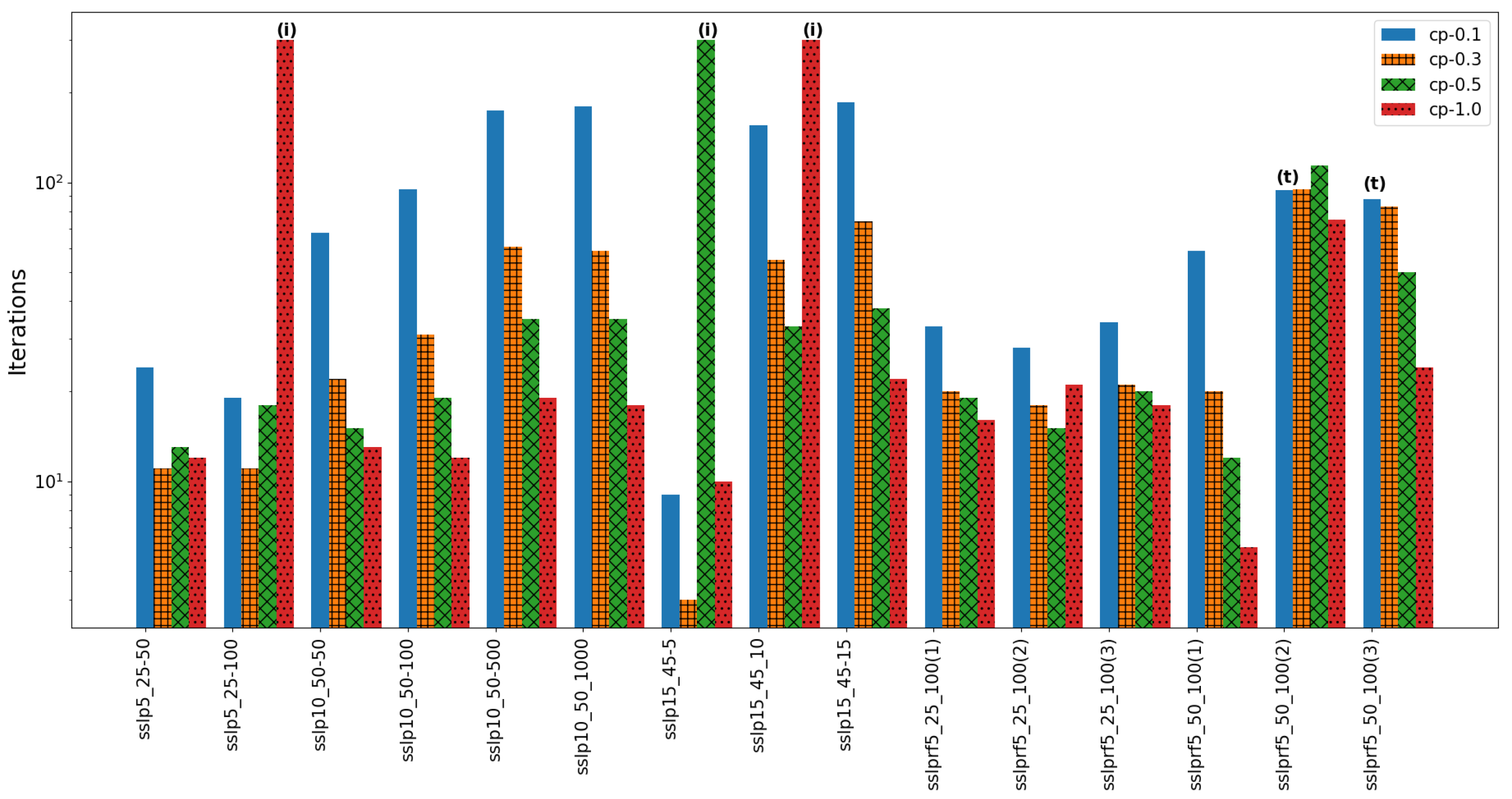
6.1.2. Computational Results for PySP

We use PySP (Pyomo 5.0.0) to solve the SSLP, SSLPR, and DCAP problems. Each subproblem is solved with the CPLEX (12.7.0) quadratic solver. We use the cost-proportional (CP) heuristic to set the values of ρ ( i ) . The multipliers α in the CP heuristic are set to 0.1, 0.3, 0.5, and 1.0, respectively. Note that the main results shown in this section are not using WW heuristics, i.e., we do not use the variable fixing and slamming, or cycle-detection heuristics. We will make a comparison of PySP with WW heuristics and PySP without WW heuristics at the end of this section.
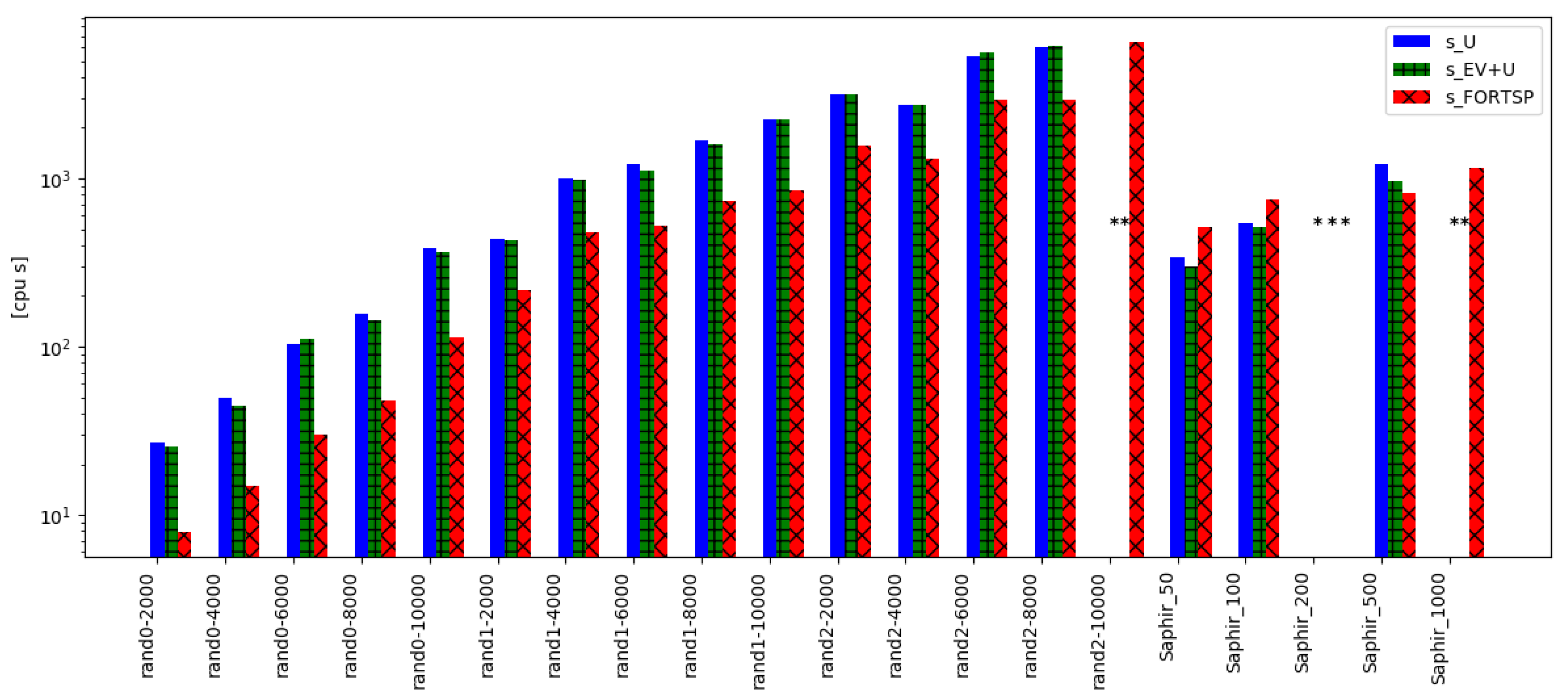
The number of iterations and the walltime for different multipliers are shown in Figure 1 and Figure 2, respectively. If the PH algorithm reaches iteration limit, there is an “(i)” label at the top of the column. If the PH algorithm reaches the time limit, there is a “(t)” label on top of the column. From Figure 1 and Figure 2, one can observe that setting the α value to 0.1 makes PH take the largest number of iterations and largest amount of walltime to converge in most of the instances, which may be due to the small step size. On the other hand, setting α to the largest value, i.e., 1.0, takes fewer iterations and less walltime than using other α values in most instances. However, it runs out of the iteration limit in two of the instances. Overall, setting α to 0.3 seems to be a robust choice because cp-0.3 always converges within a reasonable walltime and number of iterations. The details of the SSLP and SSLPR results are shown in Table A1 and Table A2 in Appendix A.
We also apply PySP to solve DCAP instances. We observe that for all the DCAP instances, PySP is unable to converge within 300 iterations. The details of the results are shown in Table A3 in Appendix A where the walltime of the upper bound for those instances is reported.We compare the upper bound obtained by PySP with those obtained by DSP in the next subsection. From this experiment, we can see that it is more difficult for PySP to solve problems with mixed-binary first-stage variables than problems with pure binary first-stage variables because it is more difficult for the continuous variables to satisfy the NACs.
Scenario bundling [66,67,68] is a technique that has been used in dual decomposition algorithms. The main idea is to dualize only “some” of the non-anticipativity constraints, rather than dualizing all of them. In other words, the individual scenario subproblems are bundled into larger subproblems in which the NACs are preserved. Ryan et al. [67] used PH with scenario bundling to solve stochastic unit commitment problems. The authors showed that with the use of scenario bundling, PH can obtain solutions with a smaller optimality gap. In order to test the effectiveness of the scenario bundling, we test several instances from the SSLP and DCAP libraries. The computational results are shown in Table 2. For each instance, we try a different number of bundles. For the SSLP instances, PH with a different number of bundles can obtain the same upper bound. However, the number of bundles has a significant impact on the computational time. For example, for SSLP_10_50 with 1000 scenarios, PH with 50 bundles can reduce the walltime of the original PH with 1000 bundles to 3%. Additionally, it only takes PH with 50 bundles one iteration to converge. For DCAP problems, PH does not converge within 300 iterations for most cases, even with scenario bundling. However, PH is able to obtain better feasible solutions with scenario bundling (see UB in Table 2).
Finally, we evaluate how the use of WW heuristics can affect the performance of PySP on the SSLP and SSLPR libraries. The results on DCAP library are omitted here since PySP does not converge for DCAP instances. The solution time improvements by using WW heuristics for each SSLP and SSLPR instance are shown in Figure 3. Note that there are three cases where the improvements are omitted in the figure: case (1)—neither PH nor PH with WW heuristics can converge in 300 iterations; case (2)—only PH-WW fails to converge in 300 iterations; and case (3)—both PH and PH-WW exceed the time limit of 3 h (10,800 CPU seconds). Using WW heuristics gives significant improvements for small cost-proportional multipliers, i.e., 0.1 and 0.3. As we have described in Table 1, PH with small multipliers usually takes more iterations to converge. Therefore, the WW heuristics can accelerate convergence for those instances, more effectively. However, there are also a few instances where PH can converge, but PH with WW heuristics cannot converge, which are denoted by case (2) in Figure 3.

6.2. DSP: Decompositions for Structured Programming

DSP [49] is an open-source software package implemented in C++ that provides different types of dual decomposition algorithms to solve stochastic mixed-integer programs (SMIPs). DSP can take SMPS files, and JuMP models as input via a Julia package Dsp.jl.

6.2.1. Algorithmic Innovations in DSP

From the description of the dual decomposition algorithm in Section 5, one can observe that the lower bounds of the dual decomposition algorithm are affected by the way the Lagrangian multipliers are updated. One advantage of DSP is that the authors have implemented different dual-search methods including the subgradient method, the cutting plane method, and a novel interior-point cutting-plane method for the Lagrangian master problem. The authors observed that if the simplex algorithm is used, the solutions to the Lagrangian master problem can oscillate significantly, especially when the Lagrangian dual function is not well approximated. Therefore, the authors proposed to solve the Lagrangian master problem suboptimally using an interior point method, which follows from the work of Mitchell [69].
The authors also proposed some tightening inequalities that are valid for the Lagrangian subproblems. These valid inequalities, including feasibility and optimality cuts, are obtained from Benders subproblems, where the integrality constraints are relaxed. Computational results show that the Benders-like cuts can be effective in practice. The latest DSP distribution is able to complete Algorithm 3 using the Dantzig–Wolfe decomposition-based branching strategy described in [51].

6.2.2. Computational Results for DSP in Comparison with PySP

We test the dual decomposition algorithm on the SSLP, SSLPR, and DCAP libraries. Each subproblem is solved with CPLEX (12.7.0) mixed-integer linear solver. The interior point method proposed by the authors [49] is used to solve the Lagrangian master problem, which is solved with CPLEX as well. Benders-like cuts are not used because the implementation of Benders cuts in DSP only works with SCIP.
In Figure 4 and Figure 5, we evaluate the best feasible solution (the upper bound) obtained by PySP, and the upper and lower bounds obtained by DSP. For each instance, we include three different gaps. The upper and lower bounds from Ref. [61] are used to evaluate the bounds from PySP and DSP. Note that the bounds from literature are close to the global optimality of each instance. The first column for each instance in both Figure 4 and Figure 5 is the gap between the upper bound from PySP ( P y S P u b ) and the lower bound from the literature ( L i t e r a t u r e l b ). The second column represents the gap between the upper bound from DSP ( D S P u b ) and the lower bound from the literature ( L i t e r a t u r e l b ). The third column represents the gap between the upper bound from literature ( L i t e r a t u r e u b ) and the lower bound from DSP ( D S P l b ).
For the SSLP and SSLPR instances shown in Figure 4, although PySP can converge within the time and iteration limit, the best feasible solution obtained from PySP ( P y S P u b ) may not be optimal. There are about 1% gaps for some of the SSLP instances (see the first column of each instance in Figure 4). DSP can solve more instances to optimality than PySP (see the second column of each instance in Figure 4). The lower bounds obtained by DSP are also quite tight, usually less than 0.01% (see the third column of each instance in Figure 4). Note that the literature values for SSLPRF5_50_100(1), SSLPRF5_50_100(2), and SSLPRF5_50_100(3) do not match the values from our experiment. Therefore, we try to solve the deterministic equivalent of these instances to obtain bounds. The literature bounds of SSLPRF5_50_100(3) come from solving the deterministic equivalent. The gaps of SSLPRF5_50_100(1) and SSLPRF5_50_100(2) are omitted since the corresponding deterministic equivalent cannot be solved within 3 h.
For the DCAP instances where we have mixed-integer first-stage variables, the best feasible solutions from PySP ( P y S P u b ) and DSP ( D S P u b ) are quite far from optimality. The gaps of the first two columns are around 10%. On the other hand, the lower bounds obtained from DSP ( D S P l b ) are tight. The gaps between ( L i t e r a t u r e u b ) and ( D S P l b ) are around 0.1%. Therefore, in order to improve the relative optimality gap of DSP, the focus should be on designing more advanced heuristics to obtain better feasible solutions.

6.3. Results from Branch-and-Bound Algorithm in DSP

As we were completing this paper, a new version of DSP [51] was developed that uses the branch-and-bound algorithm similar to Algorithm 3. We test the branch-and-bound decomposition on the SLSP, SSLPR, and DCAP test instances. The computational setting is the same as the one described in the previous section. Table 3, Table 4 and Table 5 show the results obtained by DSP. We highlight that almost all the instances were solved to optimality within the walltime limit.
In all the SSLP instances (except SSLP15_45), DSP using the DW-based branch-and-bound (DSP-DW) is able to solve the instances to optimality in times lower than the ones from the DSP implementing only the first iteration of DD. The same trend is replicated on the SSLPRF instances.
On the other hand DSP-DW is remarkably slower in attaining algorithmic convergence in the DCAP test set. This behavior can be explained by looking at the D S P l b vs. L i t e r a t u r e u b gap in Figure 4 and Figure 5. The standard implementation of DSP is able to close the optimality gap in the SSLP and SSLPR instances by solving the Lagrangian relaxation problem (15a) and using heuristics to compute a primal bound. Nonetheless, this strategy does not work in the DCAP set for which additional computation is devoted by DSP-DW to close the gap via branch-and-bound.

7. Conclusions

We presented a summary of the state-of-the-art methodologies for the solution of two-stage linear stochastic problems. First, we introduced the mathematical formulation of such programs and highlighted features in their structure, which enable the development of decomposition algorithms. These methodologies are classified in two groups: node-based decomposition and scenario-based decomposition.
For two-stage stochastic programs with continuous recourse, we summarized Benders decomposition, which partitions the problem according to its time structure. BD may present computational problems, which can be alleviated by reducing the cost of each iteration, and/or decreasing the number of iterations.
Scenario decomposition methodologies are popular alternatives in the case of (mixed) integer recourse. The progressive hedging algorithm and dual decomposition relax the nonanticipatity restrictions and provide the user with valid bounds. Our numerical results show that the performance of PH is strongly affected by the constant penalty multiplier. Furthermore, its performance and the quality of the approximate solution may be enhanced by grouping the scenarios in large bundles (or scenario sets). We also tested the dual decomposition algorithm with the DSP package. The computational results show that DSP is able to provide a tight lower bound on the instances that we tested. However, the optimality gaps can be as large as 10%, relative to the upper bound from literature. Therefore, for those tested instances, future effort should be focused on developing more advanced heuristics to improve the best feasible solution. Moreover, we tested the newest DSP implementation, which incorporates a Dantzig–Wolfe decomposition-based branch-and-bound algorithm to close the optimality gap. In most of the instances, it is able to retrieve a global solution in the given walltime limit. We highlight that its computational performance depends on the strength of the dual decomposition.
At the time we completed this paper, several new developments were made in stochastic programming software. These software packages have the capability of solving multi-stage stochastic programs, e.g., SDDP.jl [70], StochasticPrograms.jl [71], and MSPPy [72]. In the terms of algorithmic development, recent works have extended the capability to solve nonlinear problems [4,73,74,75,76,77,78]. Furthermore, it should be noted that the paper focuses on the risk-neutral setting of two-stage stochastic programs. However, the studied approaches can be easily extended to the risk-averse setting [79], e.g., by including some risk measures, such as the conditional value at risk (CVar).

Author Contributions

J.J.T. conceptualization, computational study and paper writing; C.L. conceptualization and paper writing; R.M.A. conceptualization and review; I.E.G. conceptualization, supervision and review. All authors have read and agreed to the published version of the manuscript.

Funding

This research was funded from the Center of Advanced Process Decision-making at Carnegie Mellon University.

Institutional Review Board Statement

Not applicable.

Informed Consent Statement

Not applicable.

Data Availability Statement

Not applicable.

Conflicts of Interest

The authors declare no conflict of interest.

Appendix A. Computational Results for PySP

Table A1. Computational results for PySP on SSLP.
InstancesScenarioscp MultiplierIterationsTimeUB
SSLP_5_2550cp 0.12417.59−121.60
cp 0.3118.16−121.60
cp 0.5138.53−121.60
cp 1.0127.80−121.60
100cp 0.11927.38−127.37
cp 0.31115.27−127.37
cp 0.51821.26−127.37
cp 1.0>300303.53−125.59
SSLP_10_5050cp 0.168254.15−364.64
cp 0.32271.57−364.64
cp 0.51549.19−364.64
cp 1.01341.91−364.64
100cp 0.195540.21−354.19
cp 0.331149.33−354.19
cp 0.51988.54−354.19
cp 1.01257.98−354.19
500cp 0.11744322.45−349.14
cp 0.3611265.18−349.14
cp 0.535688.90−349.14
cp 1.019379.64−349.14
1000cp 0.11809984.56−351.71
cp 0.3592849.90−357.71
cp 0.5351604.27−357.71
cp 1.018845.16−351.71
SSLP_15_455cp 0.1912.48−262.40
cp 0.345.85−261.20
cp 0.5>300197.35−261.20
cp 1.0109.65−261.20
10cp 0.1155485.38−260.50
cp 0.355108.15−260.50
cp 0.53358.23−259.30
cp 1.0>300463.63−259.30
15cp 0.11861416.21−253.60
cp 0.374286.78−253.60
cp 0.538126.79−253.60
cp 1.02265.08−253.20
Table A2. Computational results for PySP on SSLPR.
Instancescp MultiplierIterationsTimeUB
SSLPRF_5_25_100_1cp 0.133722.61−74,005.84
cp 0.320461.1−74,005.84
cp 0.519427.04−74,005.84
cp 1.016315.67−74,005.84
SSLPRF_5_25_100_2cp 0.128852.75−72,671.95
cp 0.318517.33−72,671.95
cp 0.515436.16−72,671.95
cp 1.021539.61−72,671.95
SSLPRF_5_25_100_3cp 0.134735.9−75,664.19
cp 0.321412.91−75,664.19
cp 0.520397.01−75,664.19
cp 1.018348.75−75,664.19
SSLPRF_5_50_100_1cp 0.1592457.66138,900.12
cp 0.320814.04138,900.12
cp 0.512429.35138,900.12
cp 1.06200.07138,900.12
SSLPRF_5_50_100_2cp 0.194>10,800
cp 0.3957382.14245,424.96
cp 0.51144315.02245,424.96
cp 1.0753008.51500,144.07
SSLPRF_5_50_100_3cp 0.188>10,800
cp 0.3836984.09258,578.79
cp 0.5503887.54258,578.79
cp 1.0241727.73258,578.79
Table A3. Computational results for PySP on DCAP.
InstancesScenarioscp MultiplierIterationsTimeUB
DCAP 233200cp 0.1>300456.182206.7
cp 0.3>300457.52431.8
cp 0.5>300458.231966.1
cp 1.0>300455.881952.6
300cp 0.1>300734.231862.0
cp 0.3>300726.591943.3
cp 0.5>300726.771831.6
cp 1.0>300741.171815.4
500cp 0.1>3001515.272498.1
cp 0.3>3001492.592000.0
cp 0.5>3001467.641939.2
cp 1.0>3001494.131893.8
DCAP 243200cp 0.1>300481.962465.9
cp 0.3>300478.342454.2
cp 0.5>300481.512369.3
cp 1.0>300466.952383.2
300cp 0.1>300792.012825.8
cp 0.3>300756.172802.8
cp 0.5>300710.442755.0
cp 1.0>300776.972743.1
500cp 0.1>3001690.742196.0
cp 0.3>3001622.82235.2
cp 0.5>3001674.762216.7
cp 1.0>3001536.422323.3
DCAP 332200cp 0.1>300456.581362.7
cp 0.3>300427.651529.1
cp 0.5>300450.881278.0
cp 1.0>300460.351171.0
300cp 0.1>300714.831332.1
cp 0.3>300698.521948.9
cp 0.5>300709.211904.4
cp 1.0>300706.751766.3
500cp 0.1>3001464.111768.6
cp 0.3>3001451.731822.8
cp 0.5>3001473.661846.6
cp 1.0>3001452.641861.6
DCAP 342200cp 0.1>300449.91993.4
cp 0.3>300476.771990.4
cp 0.5>300445.111870.6
cp 1.0>300470.821830.8
300cp 0.1>300722.62260.3
cp 0.3>300739.942371.1
cp 0.5>300690.762497.7
cp 1.0>300702.232255.9
500cp 0.1>3001582.92198.1
cp 0.3>3001604.982317.5
cp 0.5>3001555.92290.6
cp 1.0>3001593.412097.5

Appendix B. Computational Results for DSP

Table A4. Computational results for DSP on SSLP.
InstancesScenariosIterationsTimeLBUBGap [%]
SSLP_5_2550163.86−121.60−121.600.00
100176.00−127.37−125.591.42
SSLP_10_505057204.63−364.64−357.981.86
10044213.95−354.19−341.333.77
500692439.58−349.14−344.021.49
1000602960.55−351.71−336.234.60
SSLP_15_4551514.14−262.40−261.200.46
1041152.25−260.50−260.500.00
1544207.39−253.60−253.600.00
Table A5. Computational results for DSP on SSLPR.
InstancesIterationsTimeLBUBGap [%]
SSLPRF_5_25_100_1361239.55−74,005.84−74,005.840.00
SSLPRF_5_25_100_2381783.89−72,671.95−72,671.950.00
SSLPRF_5_25_100_3401541.41−75,664.19−75,664.190.00
SSLPRF_5_50_100_1886776.87138,900.12138,900.120.00
SSLPRF_5_50_100_2579357.49163,943.96245,427.1433.20
SSLPRF_5_50_100_385>10,800189,569.71254,469.6225.50
Table A6. Computational results for DSP on DCAP.
InstancesScenariosIterationsTimeLBUBGap [%]
DCAP 2332005917.651833.402053.7710.73
3006935.451642.731812.899.39
5006029.571735.092257.8123.15
DCAP 2432005417.812321.172447.755.17
3005023.622556.682600.561.69
5006258.242165.482481.8412.75
DCAP 3322005916.251059.091337.7120.83
3007939.581250.911431.1112.59
5006655.941587.071802.2411.94
DCAP 3422005214.321618.071804.5710.34
3004621.192065.422252.338.30
5005651.591902.982059.877.62

Appendix C. Software Packages for Benders Decomposition

In this section, we review two software packages, GAMS–DECIS [44,45] and FORTSP [46] for Benders decomposition. Both packages are benchmarked with 20 instances from the random [80] and SAPHIR [81] test collections. All of the test problems are available in the SMPS format; however, specific modifications need to be done in order to make the format compatible with DECIS. The computational experiments are performed on a Linux machine with a 2.67 GHz Intel Xeon CPU, 128 GB of RAM, and a limit of 3 h of walltime.
The random collection consists of 15 instances artificially generated with the test problem generator GENSLP [82]. The instances are grouped into three sets of problems (rand0, rand1, rand2), each one of them with five instances with 2000, 4000, 6000, 8000 and 10,000 scenarios. None of the instances represent a real-world problem; nonetheless, they are successfully used to assess the performance of stochastic solvers (see [83]). All problems in this collection present uncertainty only in the right-hand side (RHS) coefficients h ω .
The SAPHIR collection consists of five instances of the optimization of a gas-purchase portfolio, considering the cost of purchase, as well as underground storage capacities and transportation, under uncertain demand conditions [84]. In this family of problems, the random elements are located in both the RHS and constraint matrices W ω and T ω .
The sizes of all of the test problems are shown in Table A7. The size is expressed as the number of constraints (Rows) and variables (Cols) in the first stage and the second stage per scenario. None of the test instances consider integer variables in the first-stage.
Table A7. Sizes of SLP instances tested.
NameScenariosFirst StageSecond Stage
RowsColsRowsCols
rand02000, 4000, 6000, 8000, 10,000501002550
rand12000, 4000, 6000, 8000, 10,00010020050100
rand22000, 4000, 6000, 8000, 10,00015030075150
saphir50, 100, 200, 500, 1000325386783924

Appendix C.1. FortSP: A Stochastic Programming Solver

FortSP is a solver for the solution of linear and mixed-integer linear stochastic programs. It accepts input in the SMPS format, or through a separate SAMPL translator (an AMPL extension for stochastic programming). In addition, FortSP can be used as a library with an application programming interface (API) in C. FortSP enables the user to solve stochastic two-stage linear programs with four variants of Benders decomposition, and provides three different solution approximations for mixed-integer instances.

Appendix C.1.1. Algorithmic Innovations in FortSP

The innovations in FortSP for two-stage linear and mixed-integer linear stochastic programs are described by Ellison et al. [46]. FortSP incorporates five methods to solve two-stage stochastic linear programs: (i) solving the deterministic equivalent via the interior-point method (IMP), (ii) Benders decomposition with aggregated cuts (see problem (A1)), (iii) regularized decomposition [85] (see problem (12)), (iv) Benders decomposition with regularization of the expected recourse by the level method [86] (see problem (14)), and (v) the trust region (regularization) method [41] (see problem (13)).
To solve mixed-integer instances, FortSP uses the deterministic equivalent with both implicit and explicit representations for the NACs. In addition, it incorporates a specialized L-shaped algorithm based on branch-and-cut for instances with mixed-integer variables in the first-stage and continuous and complete recourse. This method might be accelerated with the variable neighborhood decomposition search heuristic (VNDS) [87].
All of the Benders variants in FortSP are formulated in the a g g r e g a t e d form shown in Equation (A1). D i s a g r e g a t e d formulations (i.e., problem (9)) store larger information in the master problem, which yields a reduction in the number of iterations. However, this is done at the expense of larger master problems. As a rule of thumb, the d i s a g g r e g a t e d approach is expected to be more effective when the number of scenarios | Ω | is not significantly larger than the number of constraints m 1 of the first-stage program [1].
( B M P ) T C d = min x , v c T x + v
s . t . A x b , x X , v R
( h j T j x ) T μ ¯ j 0 j E
ω Ω τ ω ( h ω T ω x ) T π ω k v k K

Appendix C.1.2. Computational Results for FortSP

We use FortSP to solve the random [80] and SAPHIR [81] test instances. The number of iterations and walltime for different solution methodologies are shown in Table A8, where IPM stands for interior-point method, RD for regularized decomposition, and TR for trust region. The CPLEX (12.5.1) linear and quadratic solver is used to solve the set of master problem and subproblems. For decomposition methodologies, a stopping optimality gap of 1 × 10 5 is used. FortSP automatically selects the methodology used to solve the set of master problem and recourse instances, from primal and dual simplex, as well as an interior-point method. In addition, FortSP considers the warm-start of linear programs.
From Table A8, one can observe that solving the deterministic equivalent via IPM is an effective alternative, outperforming BD in most of the instances considered; nonetheless, it fails to solve the larger instances in the SAPHIR set. Regularized decomposition and the trust region method perform better than BD in the SAPHIR set, effectively decreasing the number of iterations and the solution time. However, RD fails on the whole set of RAND test problems. Decomposition with the level method presents the best performance on both of the benchmark sets, yielding computational times close to the interior-point method and effectively reducing the number iterations of the standard BD method.
Table A8. Computational results for FortSP.
InstancesScenariosIPMBendersLevelRDTR
IterTimeIterTimeIterTimeIterTimeIterTime
rand0200012838.218010.57447.53--10313.56
40004626.186920.023211.50--8424.60
60005746.3010841.105121.53--13651.36
80006466.2812765.345034.00--15981.33
10,0008095.32230153.997153.39--311207.46
rand120003734.74391237.407452.86--502307.87
40004679.92502528.995969.90--624655.29
600047116.40385576.335894.25--484728.86
800050160.58453818.7865126.08--6111126.22
10,00051414.214301064.2552526.53--5581388.47
rand220003663.788861643.4065133.59--12392415.88
400040140.564141355.3742152.27--5731936.61
600048245.895143067.9252318.58--6754172.58
800051329.104543036.4044310.44--6814638.54
10,00051418.116866774.7552528.81--9889733.37
Saphir50--127527.0639215.722282.303377.18
100--122768.4244503.8729216.373497.01
200------30163.661984.15
500326555.35122847.1742426.2829231.102585.62
1000--1381153.4051655.6629259.2986289.53

Appendix C.2. DECIS: A System for Solving Large-Scale Stochastic Programs

DECIS is a software platform for the solution of large-scale two-stage stochastic programs. It accepts problems in SMPS format. To use DECIS in GAMS, the user needs to formulate the deterministic problem and time distribution of the constraints and variables in the GAMS interface, which automatically constructs the c o r e and t i m files. The uncertain components and realization probabilities are set from an external s t o c h a s t i c file (.sto extension in SMPS format), which is written by the user. Recent developments in GAMS allow to use the extended mathematical programming (EMP) framework to define a stochastic program for DECIS, as well as setting the optimization of two additional risk measures: value at risk (VaR) and conditional value at risk (CVaR).

Appendix C.2.1. Algorithmic Innovations in DECIS

DECIS incorporates multiple alternatives to solve linear two-stage stochastic programs, including (i) Benders decomposition with aggregated cuts, and, (ii) a regularized decomposition variant. The latter uses MINOS to solve the quadratic master problem (12), and requires the user to select a proper constant penalty parameter ( t k > 0 ). The overall algorithm performance and convergence are strongly affected by the value of t k .
When the number of realizations is large, DECIS can employ advanced Monte Carlo sampling techniques to compute good approximate solutions. Instead of considering the whole set of possible outcomes to estimate the expected cost, DECIS uses an independent sample drawn from the distribution of random parameters. In addition to crude Monte Carlo sampling, DECIS incorporates importance sampling and control variates, variance reduction techniques which enhance the estimation of the expected cost. In addition, DECIS computes a confidence interval in which the optimal objective function value lies.

Appendix C.2.2. Computational Results for DECIS

We use DECIS to solve the random and SAPHIR test instances. The number of iterations and walltime for different solution methodologies are shown in Table A9. Two initialization strategies are tested on Benders decomposition: (U) where the initial first-stage candidate solution is 0, and (EV+U) where BD is employed to solve the EV (expected value) problem. The EV optimal solution is then used as a starting point for the stochastic instance. Iter-EV and Iter-U stand for the number of iterations required to solve the EV and stochastic problem, respectively. A stopping optimality gap of 1 × 10 5 is considered. DECIS-CPLEX (12.7.0) uses primal simplex in both the MP and subproblems in Benders decomposition. DECIS-MINOS (5.6) is used in the quadratic MP and linear subproblems in regularized decomposition.
Table A9. Computational results for DECIS.
InstancesScenariosBenders (U)Benders (EV+U)RD − 1 (U)RD − 10 (U)
IterTimeIter-EVIter-UTimeIterTimeIterTime
rand020008229.72317727.985013.177218.30
40007153.77355848.494222.115830.16
6000105112.3647106120.965840.68558.83
8000121170.2538111155.615954.2310291.64
10,000229410.7640213389.04110133.2135163.31
rand12000391459.2991384448.74120264.43255551.64
40004881051.82874871031.35117448.652961175.35
60003961269.561183631158.85100533.02146781.95
80004431763.461004361688.43106679.391531004.85
10,0004492356.121154372353.02113983.681931736.57
rand220008853213.081258703225.031421147.622652620.33
40004112784.491364052786.91931696.082123879.52
60004965470.711655205764.871324196.522236981.10
80004576151.331734596277.49973631.941405224.19
10,000---------
Saphir50167362.2116380317.21----
100151568.4415183539.73----
200---------
5001381357.8310973917.47----
1000---------
To exemplify the effects of the constant penalty term on the performance of regularized decomposition, two ρ values, 1 and 10, are tested. From Table A9, it can be observed that regularized decomposition may significantly reduce the number of iterations, and thus the solution time of the overall decomposition algorithm. In addition, stronger penalization might increase the number of iterations, as it restricts the movement of the first-stage candidate to be close to the best incumbent solution. Furthermore, this methodology might present numerical issues, such as bad scaling in the master problem, which makes the algorithm stop without closing the optimality gap. For instance, regularized decomposition fails to solve the whole set of SAPHIR problems.
Using the (EV+U) initialization can accelerate the convergence of Benders decomposition. In 14 of 17 instances where BD converged, (EV+U) had fewer iterations than the (U) strategy, as well as less solution time. The reduction in the iteration number alleviates the time spent computing an appropriate starting point.

Appendix C.2.3. Computational Results for FortSP in Comparison with DECIS

From the results in the previous subsections, it can be observed that the algorithms implemented in FortSP (Table A8) outperforms the decomposition implementations in GAMS–DECIS (Table A9) in terms of solution time. The strength of FortSP resides in the use of multiple strategies that can accelerate the convergence of the standard BD algorithm and regularization solved with MINOS. In fact, we observed that the best FortSP methodology is at least 37.3 % faster than the best algorithmic implementation evaluated with DECIS for each test problem (see Figure A1). In the instances in which none of the DECIS solvers converge, the solution time is noted as 3 h of walltime.
As expected, the performance of the BD algorithm in both FortSP and DECIS behaves similarly, having a difference of fewer than 10 iterations in each test instance. Both implementations use BD with aggregated cuts but differ in the initialization procedure. However, the BD algorithm is on average two times faster in the FortSP’s implementation than DECIS’s implementation.
Figure A1. Maximum relative improvement of the solution time by using FortSP’s solvers over DECIS’s solvers.
Algorithms 15 00103 g0a1
In this particular set of instances, the most time-consuming part of the algorithm is the cumulative solution of scenario subproblems, as can be observed in Figure A2 and Figure A3, which is explained by the large number of scenario subproblems. This difference is especially pronounced in the SAPHIR group, where the recourse problem is larger than the first-stage program, in terms of constraints and variables. In most of the test instances, DECIS with initialization in the EV solution is the methodology that spends more time solving the master problem, as it uses BD to obtain a proper starting point. Following the general trend, FortSP is faster in the solution of both the master problem and the subproblems separately, indicating that differences in the implementation play an important role in the performance of the decomposition strategies. Warm-starting and automatic selection of the linear solver might contribute to the acceleration of the convergence of BD in FortSP.
Figure A2. Cumulative solution time of masters problem in BD, where **, *** means the algorithm fails to solve the instance in 10,800 CPU seconds.
Algorithms 15 00103 g0a2
Figure A3. Cumulative solution time of scenario instances in BD, where **, *** means the algorithm fails to solve the instance in 10,800 CPU seconds.
Algorithms 15 00103 g0a3

References

  1. Birge, J.R.; Louveaux, F. Introduction to Stochastic Programming; Springer Science & Business Media: Berlin/Heidelberg, Germany, 2011. [Google Scholar]
  2. Kall, P.; Wallace, S.W. Stochastic Programming; Wiley: Chichester, UK, 1996; p. xii. [Google Scholar]
  3. Garcia-Herreros, P.; Wassick, J.M.; Grossmann, I.E. Design of Resilient Supply Chains with Risk of Facility Disruptions. Ind. Eng. Chem. Res. 2014, 53, 17240–17251. [Google Scholar] [CrossRef]
  4. Li, C.; Grossmann, I.E. An improved L-shaped method for two-stage convex 0–1 mixed integer nonlinear stochastic programs. Comput. Chem. Eng. 2018, 112, 165–179. [Google Scholar] [CrossRef]
  5. Ye, Y.; Li, J.; Li, Z.; Tang, Q.; Xiao, X.; Floudas, C.A. Robust optimization and stochastic programming approaches for medium-term production scheduling of a large-scale steelmaking continuous casting process under demand uncertainty. Comput. Chem. Eng. 2014, 66, 165–185. [Google Scholar] [CrossRef]
  6. Tarhan, B.; Grossmann, I.E. A multistage stochastic programming approach with strategies for uncertainty reduction in the synthesis of process networks with uncertain yields. Comput. Chem. Eng. 2008, 32, 766–788. [Google Scholar] [CrossRef]
  7. Van Slyke, R.; Wets, R. L-Shaped Linear Programs with Applications to Optimal Control and Stochastic Programming. SIAM J. Appl. Math. 1969, 17, 638–663. [Google Scholar] [CrossRef]
  8. Geoffrion, A.M. Lagrangean relaxation for integer programming. In Approaches to Integer Programming; Springer: Berlin/Heidelberg, Germany, 1974; pp. 82–114. [Google Scholar]
  9. Rockafellar, R.T.; Wets, R.J.B. Scenarios and Policy Aggregation in Optimization under Uncertainty. Math. Oper. Res. 1991, 16, 119–147. [Google Scholar] [CrossRef] [Green Version]
  10. Küçükyavuz, S.; Sen, S. An introduction to two-stage stochastic mixed-integer programming. In Leading Developments from INFORMS Communities; INFORMS: Catonsville, MD, USA, 2017; pp. 1–27. [Google Scholar]
  11. Lara, C.L.; Siirola, J.D.; Grossmann, I.E. Electric power infrastructure planning under uncertainty: Stochastic dual dynamic integer programming (SDDiP) and parallelization scheme. Optim. Eng. 2020, 21, 1243–1281. [Google Scholar] [CrossRef]
  12. Beltrán, F.; Finardi, E.C.; de Oliveira, W. Two-stage and multi-stage decompositions for the medium-term hydrothermal scheduling problem: A computational comparison of solution techniques. Int. J. Electr. Power Energy Syst. 2021, 127, 106659. [Google Scholar] [CrossRef]
  13. Colonetti, B.; Finardi, E.C.; de Oliveira, W. A Mixed-Integer and Asynchronous Level Decomposition with Application to the Stochastic Hydrothermal Unit-Commitment Problem. Algorithms 2020, 13, 235. [Google Scholar] [CrossRef]
  14. Li, C.; Grossmann, I.E. A review of stochastic programming methods for optimization of process systems under uncertainty. Front. Chem. Eng. 2021, 34. [Google Scholar] [CrossRef]
  15. Li, C.; Eason, J.P.; Drouven, M.G.; Grossmann, I.E. Shale gas pad development planning under price uncertainty. AIChE J. 2020, 66, e16933. [Google Scholar] [CrossRef]
  16. Ruszczyński, A. Decomposition methods in stochastic programming. Math. Program. 1997, 79, 333–353. [Google Scholar] [CrossRef]
  17. Carøe, C.C.; Schultz, R. Dual decomposition in stochastic integer programming. Oper. Res. Lett. 1999, 24, 37–45. [Google Scholar] [CrossRef]
  18. Lim, C.; Cochran, J.J.; Cox, L.A.; Keskinocak, P.; Kharoufeh, J.P.; Smith, J.C. Relationship among Benders, Dantzig–Wolfe, and Lagrangian Optimization. In Wiley Encyclopedia of Operations Research and Management Science; John Wiley & Sons, Inc.: Hoboken, NJ, USA, 2010. [Google Scholar] [CrossRef]
  19. Benders, J.F. Partitioning procedures for solving mixed-variables programming problems. Numer. Math. 1962, 4, 238–252. [Google Scholar] [CrossRef]
  20. Geoffrion, A.M. Generalized Benders decomposition. J. Optim. Theory Appl. 1972, 10, 237–260. [Google Scholar] [CrossRef]
  21. Hooker, J.N.; Ottosson, G. Logic-based Benders decomposition. Math. Program. 2003, 96, 33–60. [Google Scholar] [CrossRef]
  22. Sherali, H.D.; Fraticelli, B.M.P. A modification of Benders’ decomposition algorithm for discrete subproblems: An approach for stochastic programs with integer recourse. J. Glob. Optim. 2002, 22, 319–342. [Google Scholar] [CrossRef]
  23. Gade, D.; Küçükyavuz, S.; Sen, S. Decomposition algorithms with parametric Gomory cuts for two-stage stochastic integer programs. Math. Program. 2014, 144, 39–64. [Google Scholar] [CrossRef]
  24. Zhang, M.; Kucukyavuz, S. Finitely convergent decomposition algorithms for two-stage stochastic pure integer programs. SIAM J. Optim. 2014, 24, 1933–1951. [Google Scholar] [CrossRef] [Green Version]
  25. Ahmed, S.; Tawarmalani, M.; Sahinidis, N.V. A finite branch-and-bound algorithm for two-stage stochastic integer programs. Math. Program. 2004, 100, 355–377. [Google Scholar] [CrossRef]
  26. Rahmaniani, R.; Crainic, T.G.; Gendreau, M.; Rei, W. The Benders decomposition algorithm: A literature review. Eur. J. Oper. Res. 2016, 259, 801–817. [Google Scholar] [CrossRef]
  27. Magnanti, T.L.; Wong, R.T. Accelerating Benders decomposition: Algorithmic enhancement and model selection criteria. Oper. Res. 1981, 29, 464–484. [Google Scholar] [CrossRef]
  28. Geoffrion, A.M.; Graves, G.W. Multicommodity distribution system design by Benders decomposition. Manag. Sci. 1974, 20, 822–844. [Google Scholar] [CrossRef]
  29. Naoum-Sawaya, J.; Elhedhli, S. An interior-point Benders based branch-and-cut algorithm for mixed integer programs. Ann. Oper. Res. 2013, 210, 33–55. [Google Scholar] [CrossRef]
  30. Vanderbeck, F.; Wolsey, L.A. Reformulation and Decomposition of Integer Programs; Springer: Berlin/Heidelberg, Germany, 2009. [Google Scholar]
  31. Zaourar, S.; Malick, J. Quadratic Stabilization of Benders Decomposition. Available online: https://hal.archives-ouvertes.fr/hal-01181273/document (accessed on 15 January 2022).
  32. McDaniel, D.; Devine, M. A modified Benders’ partitioning algorithm for mixed integer programming. Manag. Sci. 1977, 24, 312–319. [Google Scholar] [CrossRef]
  33. Costa, A.M.; Cordeau, J.F.; Gendron, B.; Laporte, G. Accelerating Benders decomposition with heuristic master problem solutions. Pesqui. Oper. 2012, 32, 3–20. [Google Scholar] [CrossRef] [Green Version]
  34. Raidl, G.R.; Baumhauer, T.; Hu, B. Speeding up logic-based Benders’ decomposition by a metaheuristic for a bi-level capacitated vehicle routing problem. In International Workshop on Hybrid Metaheuristics; Springer: Berlin/Heidelberg, Germany, 2014; pp. 183–197. [Google Scholar]
  35. Holmberg, K. On using approximations of the Benders master problem. Eur. J. Oper. Res. 1994, 77, 111–125. [Google Scholar] [CrossRef]
  36. Zakeri, G.; Philpott, A.B.; Ryan, D.M. Inexact cuts in Benders decomposition. SIAM J. Optim. 2000, 10, 643–657. [Google Scholar] [CrossRef]
  37. Birge, J.R.; Louveaux, F.V. A multicut algorithm for two-stage stochastic linear programs. Eur. J. Oper. Res. 1988, 34, 384–392. [Google Scholar] [CrossRef] [Green Version]
  38. Saharidis, G.K.; Minoux, M.; Ierapetritou, M.G. Accelerating Benders method using covering cut bundle generation. Int. Trans. Oper. Res. 2010, 17, 221–237. [Google Scholar] [CrossRef]
  39. Van Roy, T.J. Cross decomposition for mixed integer programming. Math. Program. 1983, 25, 46–63. [Google Scholar] [CrossRef]
  40. Ruszczyński, A.; Świȩtanowski, A. Accelerating the regularized decomposition method for two stage stochastic linear problems. Eur. J. Oper. Res. 1997, 101, 328–342. [Google Scholar] [CrossRef]
  41. Linderoth, J.; Wright, S. Decomposition Algorithms for Stochastic Programming on a Computational Grid. Comput. Optim. Appl. 2003, 24, 207–250. [Google Scholar] [CrossRef]
  42. Zehtabian, S.; Bastin, F. Penalty Parameter Update Strategies in Progressive Hedging Algorithm. Available online: https://www.cirrelt.ca/documentstravail/cirrelt-2016-12.pdf (accessed on 15 January 2022).
  43. Hiriart-Urruty, J.B.; Lemaréchal, C. Convex Analysis and Minimization Algorithms II; Springer Science & Business Media: Berlin/Heidelberg, Germany, 2013; Volume 305. [Google Scholar]
  44. Bussieck, M.R.; Meeraus, A. General Algebraic Modeling System (GAMS). In Modeling Languages in Mathematical Optimization; Volume 88, Applied Optimization; Kallrath, J., Ed.; Springer: Berlin/Heidelberg, Germany, 2004; pp. 137–157. [Google Scholar]
  45. Infanger, G. GAMS/DECIS User’S Guide. Available online: https://www.gams.com/docs/DECIS-Users_Guide.pdf (accessed on 15 January 2022).
  46. Ellison, F.; Mitra, G.; Zverovich, V. FortSP: A Stochastic Programming Solver. Available online: https://citeseerx.ist.psu.edu/viewdoc/download?doi=10.1.1.178.5858&rep=rep1&type=pdf (accessed on 15 January 2022).
  47. Guignard, M. Lagrangean relaxation. Top 2003, 11, 151–200. [Google Scholar] [CrossRef]
  48. Kim, K.; Petra, C.G.; Zavala, V.M. An asynchronous bundle-trust-region method for dual decomposition of stochastic mixed-integer programming. SIAM J. Optim. 2019, 29, 318–342. [Google Scholar] [CrossRef]
  49. Kim, K.; Zavala, V.M. Algorithmic innovations and software for the dual decomposition method applied to stochastic mixed-integer programs. Math. Program. Comput. 2017, 10, 225–226. [Google Scholar] [CrossRef]
  50. Mitra, S.; Garcia-Herreros, P.; Grossmann, I.E. A cross-decomposition scheme with integrated primal–dual multi-cuts for two-stage stochastic programming investment planning problems. Math. Program. 2016, 157, 95–119. [Google Scholar] [CrossRef]
  51. Kim, K.; Dandurand, B. Scalable branching on dual decomposition of stochastic mixed-integer programming problems. Math. Program. Comput. 2022, 14, 1–41. [Google Scholar] [CrossRef]
  52. Watson, J.P.; Woodruff, D.L. Progressive hedging innovations for a class of stochastic mixed-integer resource allocation problems. Comput. Manag. Sci. 2011, 8, 355–370. [Google Scholar] [CrossRef]
  53. Lubin, M.; Martin, K.; Petra, C.G.; Sandıkçı, B. On parallelizing dual decomposition in stochastic integer programming. Oper. Res. Lett. 2013, 41, 252–258. [Google Scholar] [CrossRef]
  54. Gabay, D.; Mercier, B. A Dual Algorithm for the Solution of Non Linear Variational Problems via Finite Element Approximation; Institut de Recherche d’Informatique et d’Automatique: Le Chesnay-Rocquencourt, France, 1975.
  55. Eckstein, J.; Bertsekas, D.P. On the Douglas—Rachford splitting method and the proximal point algorithm for maximal monotone operators. Math. Program. 1992, 55, 293–318. [Google Scholar] [CrossRef] [Green Version]
  56. Gade, D.; Hackebeil, G.; Ryan, S.M.; Watson, J.P.; Wets, R.J.B.; Woodruff, D.L. Obtaining lower bounds from the progressive hedging algorithm for stochastic mixed-integer programs. Math. Program. 2016, 157, 47–67. [Google Scholar] [CrossRef] [Green Version]
  57. Gonçalves, R.E.C.; Finardi, E.C.; da Silva, E.L. Applying different decomposition schemes using the progressive hedging algorithm to the operation planning problem of a hydrothermal system. Electr. Power Syst. Res. 2012, 83, 19–27. [Google Scholar] [CrossRef]
  58. Boland, N.; Christiansen, J.; Dandurand, B.; Eberhard, A.; Linderoth, J.; Luedtke, J.; Oliveira, F. Combining Progressive Hedging with a Frank–Wolfe Method to Compute Lagrangian Dual Bounds in Stochastic Mixed-Integer Programming. SIAM J. Optim. 2018, 28, 1312–1336. [Google Scholar] [CrossRef] [Green Version]
  59. Guo, G.; Hackebeil, G.; Ryan, S.M.; Watson, J.P.; Woodruff, D.L. Integration of progressive hedging and dual decomposition in stochastic integer programs. Oper. Res. Lett. 2015, 43, 311–316. [Google Scholar] [CrossRef] [Green Version]
  60. Watson, J.P.; Woodruff, D.L.; Hart, W.E. PySP: Modeling and solving stochastic programs in Python. Math. Program. Comput. 2012, 4, 109–149. [Google Scholar] [CrossRef]
  61. Ahmed, S.; Garcia, R.; Kong, N.; Ntaimo, L.; Parija, G.; Qiu, F.; Sen, S. SIPLIB: A Stochastic Integer Programming Test Problem Library. 2004. Available online: https://www2.isye.gatech.edu/~sahmed/siplib/ (accessed on 10 March 2022).
  62. Ntaimo, L.; Sen, S. The million-variable “march” for stochastic combinatorial optimization. J. Glob. Optim. 2005, 32, 385–400. [Google Scholar] [CrossRef] [Green Version]
  63. Ntaimo, L. Disjunctive decomposition for two-stage stochastic mixed-binary programs with random recourse. Oper. Res. 2010, 58, 229–243. [Google Scholar] [CrossRef] [Green Version]
  64. Ahmed, S.; Garcia, R. Dynamic capacity acquisition and assignment under uncertainty. Ann. Oper. Res. 2003, 124, 267–283. [Google Scholar] [CrossRef] [Green Version]
  65. Hart, W.E.; Laird, C.D.; Watson, J.P.; Woodruff, D.L.; Hackebeil, G.A.; Nicholson, B.L.; Siirola, J.D. Pyomo-Optimization Modeling in Python; Springer: Berlin/Heidelberg, Germany, 2012; Volume 67. [Google Scholar]
  66. Gupta, V.; Grossmann, I.E. A new decomposition algorithm for multistage stochastic programs with endogenous uncertainties. Comput. Chem. Eng. 2014, 62, 62–79. [Google Scholar] [CrossRef] [Green Version]
  67. Ryan, S.M.; Wets, R.J.B.; Woodruff, D.L.; Silva-Monroy, C.; Watson, J.P. Toward scalable, parallel progressive hedging for stochastic unit commitment. In Proceedings of the 2013 IEEE Power & Energy Society General Meeting, Vancouver, BC, Canada, 21–25 July 2013; pp. 1–5. [Google Scholar]
  68. Escudero, L.F.; Garín, M.A.; Unzueta, A. Scenario cluster Lagrangean decomposition for risk averse in multistage stochastic optimization. Comput. Oper. Res. 2017, 85, 154–171. [Google Scholar] [CrossRef]
  69. Mitchell, J.E. Computational experience with an interior point cutting plane algorithm. SIAM J. Optim. 2000, 10, 1212–1227. [Google Scholar] [CrossRef] [Green Version]
  70. Dowson, O.; Kapelevich, L. SDDP. jl: A Julia package for stochastic dual dynamic programming. INFORMS J. Comput. 2021, 33, 27–33. [Google Scholar] [CrossRef]
  71. Biel, M.; Johansson, M. Efficient stochastic programming in Julia. INFORMS J. Comput. 2022. [Google Scholar] [CrossRef]
  72. Ding, L.; Ahmed, S.; Shapiro, A. A python Package for Multi-Stage Stochastic Programming. Available online: http://www.optimization-online.org/DB_FILE/2019/05/7199.pdf (accessed on 15 March 2022).
  73. Li, C.; Grossmann, I.E. A finite ϵ-convergence algorithm for two-stage stochastic convex nonlinear programs with mixed-binary first and second-stage variables. J. Glob. Optim. 2019, 75, 921–947. [Google Scholar] [CrossRef]
  74. Li, C.; Grossmann, I.E. A generalized Benders decomposition-based branch and cut algorithm for two-stage stochastic programs with nonconvex constraints and mixed-binary first and second stage variables. J. Glob. Optim. 2019, 75, 247–272. [Google Scholar] [CrossRef]
  75. Li, C.; Bernal, D.E.; Furman, K.C.; Duran, M.A.; Grossmann, I.E. Sample average approximation for stochastic nonconvex mixed integer nonlinear programming via outer-approximation. Optim. Eng. 2021, 22, 1245–1273. [Google Scholar] [CrossRef]
  76. Cao, Y.; Zavala, V.M. A scalable global optimization algorithm for stochastic nonlinear programs. J. Glob. Optim. 2019, 75, 393–416. [Google Scholar] [CrossRef]
  77. Füllner, C.; Rebennack, S. Non-convex nested Benders decomposition. Math. Program. 2022, 1–38. [Google Scholar] [CrossRef]
  78. de Oliveira, W. Regularized optimization methods for convex MINLP problems. Top 2016, 24, 665–692. [Google Scholar] [CrossRef] [Green Version]
  79. Rockafellar, R.T. Solving stochastic programming problems with risk measures by progressive hedging. Set-Valued Var. Anal. 2018, 26, 759–768. [Google Scholar] [CrossRef]
  80. Kall, P.; Mayer, J. On testing SLP codes with SLP-IOR. In New Trends in Mathematical Programming; Springer: Berlin/Heidelberg, Germany, 1998; pp. 115–135. [Google Scholar]
  81. Konig, D.; Suhl, L.; Koberstein, A. Optimierung des Gasbezugs im liberalisierten Gasmarkt unter Berucksichtigung von Rohren-und Untertagespeichern. VDI BERICHTE 2007, 2018, 83. [Google Scholar]
  82. Keller, E. GENSLP: A Program for Generating Input for Stochastic Linear Programs with Complete Fixed Recourse; Manuscript; IOR, University of Zurich: Zurich, Switzerland, 1984. [Google Scholar]
  83. Zverovich, V.; Fábián, C.I.; Ellison, E.F.; Mitra, G. A computational study of a solver system for processing two-stage stochastic LPs with enhanced Benders decomposition. Math. Program. Comput. 2012, 4, 211–238. [Google Scholar] [CrossRef]
  84. Koberstein, A.; Lucas, C.; Wolf, C.; König, D. Modeling and optimizing risk in the strategic gas-purchase planning problem of local distribution companies. J. Energy Mark. 2011, 4, 47. [Google Scholar] [CrossRef]
  85. Ruszczyński, A. A regularized decomposition method for minimizing a sum of polyhedral functions. Math. Program. 1986, 35, 309–333. [Google Scholar] [CrossRef]
  86. Lemaréchal, C.; Nemirovskii, A.; Nesterov, Y. New variants of bundle methods. Math. Program. 1995, 69, 111–147. [Google Scholar] [CrossRef] [Green Version]
  87. Hansen, P.; Mladenović, N.; Perez-Britos, D. Variable Neighborhood Decomposition Search. J. Heuristics 2001, 7, 335–350. [Google Scholar] [CrossRef]
Figure 1. Number of iterations for PH to solve SSLP instances using different cost proportional multipliers.
Algorithms 15 00103 g001
Figure 2. Walltime for PH to solve SSLP instances using different cost proportional multipliers.
Algorithms 15 00103 g002
Figure 3. Solution time improvement by using WW heuristics for SSLP and SSLPR instances.
Algorithms 15 00103 g003
Figure 4. Comparison of optimality gaps from PySP, DSP, and literature for SSLP and SSLPR library—instances with only binary in the first stage.
Algorithms 15 00103 g004
Figure 5. Comparison of the optimality gaps from PySP, DSP, and literature for DCAP library—instances with mixed-integer variables in the first stage.
Algorithms 15 00103 g005
Table 1. The sizes of the problems tested.
NameScenariosFirst StageSecond Stage
RowsColsIntsRowsColsInts
sslp_5_2550, 10015530130125
sslp_10_5050, 100, 500, 10001101060510500
sslp_15_455, 10, 151151560690675
sslprf_5_2510015530130125
sslprf_5_501001101060510500
dcap 233200, 300, 5006126152727
dcap 243200, 300, 5006126183636
dcap 332200, 300, 5006126122424
dcap 342200, 300, 5006126143232
Table 2. Computational results for PySP with scenario bundling.
InstancesScenariosBundlesIterationsTimeUB
SSLP_5_25501043.73−121.60
502417.59−121.60
1001023.99−127.37
50710.03−127.37
SSLP_10_505010430.55−364.64
5068254.15−364.64
10010283.67−354.19
5049263.59−354.19
10095540.21−354.19
500101476.13−349.13
502162.54−349.14
5001744322.45−349.14
10001017137.61−351.71
501313.07−351.71
10001809984.56−351.71
DCAP23320010>300342.971854.36
50>300232.211861.63
200>300456.182206.68
30010147>10,800
50>300317.281679.80
300>3001515.272498.12
50010>300634.601749.87
50>300400.591858.98
500>3001494.131893.83
Table 3. Results of DSP with DW-based branch-and-bound on SSLP instances.
InstancesScenariosTimeSolution
SSLP5_25501.70−121.6
1003.16−127.37
SSLP10_5050103.9−364.64
100101.62−364.191
5001110.64−349.136
10003021.83−351.711
SSLP15_45511.22−262.4
10151.79−260.5
15377.65−253.601
Table 4. Results of DSP with DW Branch-and- Bound on SSLPRF instances.
InstancesTimeLBUBGAP [%]
SSLPRF_5_25_100_1697.74−74,005.8−74,005.80
SSLPRF_5_25_100_21021.76−72,675−72,6750
SSLPRF_5_25_100_3673.04−75,666.9−75,666.90
SSLPRF_5_50_100_13071.82138,900138,9000
SSLPRF_5_50_100_29083.39163,931163,9310
SSLPRF_5_50_100_3----
Table 5. Results of DSP with DW Branch-and- Bound on DCAP instances.
InstancesScenariosTimeLBUBGAP [%]
DCAP233200417.081834.571834.570
300512.971644.251644.250
500898.051834.571834.570
DCAP243200370.682322.52322.50
300525.912559.192559.190
5001523.612167.42167.40
DCAP332200949.641060.751060.750
3001379.981252.771252.770
500-1588.6601589.2030.03
DCAP3422002732.971619.611619.610
3001970.752067.52067.50
5003958.251904.741904.740
Publisher’s Note: MDPI stays neutral with regard to jurisdictional claims in published maps and institutional affiliations.

