1. Introduction
Deep learning is a machine learning technique that teaches computers and devices logical functioning. It is inspired by the structure of the human brain. Deep learning originated as artificial neural networks (ANNs) and has developed far more efficiency after decades of research and development compared to the other machine learning algorithms [
1].
In the early stages of the development of neural networks, researchers aspired to create a system that mimicked the functions of the human brain. In 1943, McCulloch and Pitts attempted to explain how the brain could create highly complex patterns by using neurons [
2]. They invented the MCP (McCulloch Pitts neuron) model, which had a significant impact on the development of artificial neural networks. They implemented threshold logic in their model to simulate the human thought process but not to learn. Since then, the development of deep learning has been slow but steady, with several significant milestones along the way. In 1958, Frank Rosenblatt invented the perceptron, the first prototype of our modern neural networks, which consisted of two layers of processing units that are commonly thought of as a basic mechanism for recognizing simple patterns [
3]. Rather than undergoing further development and research, the evolutionary history of neural networks and artificial intelligence underwent a winter after 1969, after the MIT professors Minsky and Papert proved the limitations and failings of the perceptron [
4].
The standstill was broken when the backpropagation algorithm emerged in 1974, invented by Werbos [
5]. It is considered a significant milestone in neural network development. In 1980, Fukushima [
6] introduced the “Neocognitron,” which is regarded as the ancestor of convolutional neural networks, followed by the Boltzmann machine, invented by Hinton et al. in 1985 [
1], and the recurrent neural network, invented in 1986 by Jordan [
7]. In 1998, Yan LeCun introduced the convolutional neural network with backpropagation for document analysis [
8]. Deep learning has made major progress since 2006, when Hinton introduced the concept of deep belief networks (DBNs) [
9,
10]. These involve a two-stage plan: pre-training and fine-tuning. This technique allowed researchers to train neural networks much more deeply than previous methods.
Deep learning algorithms aim to draw similar conclusions as humans do by continuously analyzing data according to a given logical structure. Deep learning allows machines to manipulate images, text, or audio files like humans to accomplish human-like tasks. To achieve this, deep learning uses a multi-layered structure of algorithms called neural networks. As the name suggests, deep learning involves going deep into multiple layers of a network, which include a hidden layer. As one goes deeper, more complex information is extracted. Deep learning relies on iterative learning methods, which expose machines to very large datasets. It helps computers to learn to identify traits and adjust to changes. Machines are able to learn differences among datasets, understand the logic, and reach reliable conclusions after repeated exposures [
1].
A review on deep learning has been presented in [
11]. In [
11], the following information is provided: Computational models consist of multiple layers for processing. They are permitted to learn data representations with various levels for abstraction by deep learning. By using these techniques, the state-of-the-art has been enhanced in several fields, including visual object recognition, speech recognition, genomics, and discovery of drugs, along with plenty of others. Backpropagation is applied by deep learning in order to find the complex structure within a huge dataset, and this for specifying the way that internal parameters of machine have to be altered by the machine, and these are employed to calculate the representation within every layer depending on the representation within the prior layer. RNNs are mainly used for sequential data, such as speech and text, whereas CNNs are used for the processing of images, speech, audio, and video.
In recent years, a large number of studies, such as [
9,
10,
11,
12], have made use of deep learning and demonstrated its capabilities in many respects, including healthcare and health informatics, such as in bioinformatics, medical imaging, pervasive sensing, medical informatics, and public health [
13,
14,
15,
16,
17,
18,
19,
20,
21,
22,
23,
24,
25]; motor imagery classification [
26], for the performance improvement of sensorless FOC [
27]; and a new method developed for a retrofitted self-tuned controller with FPGA [
28] and for a self-tuning neural network PID [
29].
This paper aims to provide a literature review on different well-known deep learning algorithms. We highlight their capabilities, suitabilities, shortcomings, and applications, which many researchers in this field can benefit from knowing. Moreover, critical analyses of different deep learning algorithms are provided, focusing in particular on their advantages, disadvantages, and applications, whether supervised or unsupervised. In addition, the application of deep learning algorithms to healthcare is also introduced.
The main contribution of this paper is to systematically review several popular deep learning algorithms such as backpropagation, autoencoders, variational autoencoders, restricted Boltzmann machines, deep belief networks, convolutional neural networks, recurrent neural networks, generative adversarial networks, capsnets, transformer, embeddings from language models, bidirectional encoder representations from transformers, and attention in natural language processing. This review discusses several challenges of deep learning. This literature review also demonstrates the advantages, disadvantages, and applications of these the algorithms, and identifies whether they are supervised or non-supervised. Moreover, the applications of deep learning algorithms in healthcare are also presented; for instance, details of how deep learning algorithms can be used to fight COVID-19 pandemic are provided in this paper. The directions of future works are also given in this paper.
The researchers in the deep learning field interested in using deep learning algorithms in healthcare can obtain benefits from this review, which provides detailed information about each algorithm. In addition, beginners and new researchers in the deep learning field can read this review as a starting point to gain a comprehensive understanding of each given deep learning algorithm, helping them to attain the knowledge that they need to solve problems related to deep learning and to design and develop deep learning algorithms.
The paper is organized as follows: Works related to deep learning algorithms are presented in
Section 2, followed by a comparison of the accuracy of deep learning algorithms applied in different domains. Artificial neural networks and several well-known deep learning algorithms are introduced in
Section 3. A comparison between these deep learning algorithms based their advantages, disadvantages, applications, and whether they are supervised or unsupervised is presented in
Section 4. The application of deep learning algorithms to healthcare is given in
Section 5. Several challenges of deep learning are displayed in
Section 6. Future directions of deep learning are provided in
Section 7. Finally, conclusions and future works are introduced in
Section 8.
2. Related Works
Deep learning has been widely implemented in various areas in health informatics, such as bioinformatics, medical imaging, pervasive sensing, medical informatics, and public health [
9]. An analysis of deep learning algorithms reported in the literature related to the health sector, especially COVID-19 prediction, classification, and detection strategies is presented below. Deep learning is able to be employed reliably with respect to physiological signals obtained via electromyogram (EMG), electroencephalogram (EEG), electrooculogram (EOG), or electrocardiogram (ECG). For these purposes, the most common algorithms used in processing these physiological signals are RNNs and one-dimensional CNNs [
9].
The author of [
12] proposed a sonar target recognition. Two-layer backpropagation networks are trained to distinguish between reflected sonar signals from rocks and metal cylinders at the bottom of the Chesapeake Bay. A total of 60 input units and 2 output units are involved. The input pattern is based on the Fourier transform of the raw time signal. The best performance was obtained with 12 hidden units (nearly 100% training set accuracy).
The authors of [
30] proposed a solution for medical practitioners handling a COVID-19 crisis that implements protocols of investigation for the first patient infected by this disease, which will also be beneficial to epidemiologists for making a decision about virus spread. This paper presents a framework based on deep learning (specifically, stacked auto-encoders in medical image retrieval) in its feature-extraction phase. During retrieval tasks, this method reduces the image’s size to a small, compact representation, allowing for faster image comparisons. In a content-based image retrieval system, the importance of the auto-encoder approach can be seen, since it achieves good recognition accuracy at 80% for COVID-19 digital images, given the capability of the stacked encoders. Autoencoder algorithms have also been developed for cancer diagnosis. Sparse autoencoders are presented for microaneurysm detection in fundus images as a part of a diabetic retinopathy strategy. Additionally, various autoencoder-based learning methods have been developed for use in Alzheimer’s disease prediction based on functional magnetic resonance images (FMRI), 3D brain reconstruction, cell clustering, and human behavior monitoring [
31]. In [
13], researchers examined various autoencoding architectures that integrated multiple types of data (e.g., multi-omic and clinical) from cancer patients. They explored these approaches and provided a clear framework for developing systems which can be used for investigating cancer characteristics and translating some of the results into clinical applications. Using these networks, they described how to design, build, and apply integrative analyses of heterogeneous data on breast cancer. These approaches yield accurate and stable diagnoses by producing relevant data representations.
RBM architectures can be applied to manifold brain MRIs used in Alzheimer disease detection, segmenting multiple sclerosis lesions in multi-channel 3D MRIs, assigning diagnosis automatically according to the clinical status of patients, suicide risk prediction for mental health patients using low-dimensional approaches to the medical aspects embedded in electronic health records (EHRs), and determining photoplethysmography signals for health monitoring [
14]. A deep learning framework for the classification of complex hyperspectral medical images is presented in this study. To accomplish this, a deep Boltzmann machine (DBM) architecture of the bipartite structure was developed as an unsupervised generative model. The implementation is based on a three-layer unsupervised network with a backpropagation structure. In the present dataset, image patches are collected and classified into two classes, namely, non-informative and discriminative classes. The spatial information is used for classification and spectral-spatial representations of class labels are created. The accuracy, false-positive predictions, and sensitivity are calculated for the fully-connected network based on the labelled classes. With the proposed cognitive computation technique, an accuracy of 95.5% and sensitivity of 93.5% were achieved. The DBM model provides a significant improvement in the computer-aided diagnosis of cancerous regions in HIS (hyperspectral imaging) images. This method separates two types of image patches, informative and non-discriminative, in the first phase. By calculating the accuracy and success rate of DBM in the second phase of learning, the performance was confirmed. This method was 6.1% more accurate than CNN. The results showed that the unsupervised DBM was best suited for identifying cancer regions from complicated 3D hyperspectral images [
15].
DBNs are used in the modeling of compound–protein interactions, anomaly detection, biological parameter monitoring, obstacle detection, sign language recognition, detecting lifestyle diseases, and modeling infectious disease epidemics [
31]. In [
16], deep belief networks were used to classify normal and COVID-19 patients using medical images of chest X-rays. The proposed system successfully identifies COVID-19 cases with a 90% accuracy rate. The diagnosis is usually based on the presence of a white patchy shadow in the lungs. By using a Gaussian filter (to remove the noise), it is able to detect these diseases through these medical images. The medical images are then separated by separating the important section of the lungs from the others. Threshold-based segmentation is performed to separate gray pixels from the others, and the number of gray pixels in lungs affected by COVID-19 is very low in comparison to normal lungs.
CNN algorithms can be employed in the prediction of risk of osteoarthritis by using the automatic segmentation of knee cartilage MRIs, when using retinal fundus photographs to detect diabetic retinopathy, in dermatologist-level classification of skin cancer, in congestive heart failure prediction, for predicting chronic obstructive pulmonary disease using longitudinal EHRs, for predicting the quality of sleep using physical activity data during awake time, in electroencephalogram analysis, and for estimating the prevalences of various chromatin marks [
14]. The early stages of Alzheimer’s disease (AD) are associated with mild cognitive impairment (MCI).
For the early diagnosis of Alzheimer’s disease, some authors proposed a new voxel-based hierarchical feature extraction method (VHFE). The entire brain was divided into 90 regions of interest (ROIs) using an automatic anatomical labeling template (AAL). They divided the uninformative data by selecting the informative voxels in each ROI, using a baseline of the voxels’ values to make a vector. On the basis of the correlations between voxels of different groups, the features for the first stage were selected. In order to learn deeply hidden features, the brain feature maps made up of the voxels of each subject were fed into a convolutional neural network (CNN). The results show that the proposed method is robust, having a promising performance in comparison to the current state-of-the-art methods [
18].
In [
32], processing data that exhibit natural spatial invariance (e.g., images whose meanings do not change under translation) is shown to have grown to be central in the field (CV) [
32]. The use of deep learning systems could help physicians by providing second opinions and flagging concern areas. In object-classification, CNNs learn to classify objects contained an images and have achieved human-level performance. They are initially trained on a massive dataset, unrelated to the task of interest, to learn the natural statistics in images (curves, straight lines, colorations, etc.) before being further fine-tuned on a much smaller dataset related to the task of interest (e.g., medical images). The higher-level layers of the algorithm are retrained to distinguish between diagnostic cases. CNNs demonstrated strong performance in transferring learning [
33]. Clinicians have started to utilize image segmentation and object detection for urgent and easily missed cases, such as identifying large-arteria occlusions in the brain using radiological images [
19], during which severe brain damage may occur in a short period of time (a few minutes). Moreover, cancer histopathology reading can be supplemented with CNNs trained to detect mitotic cells [
20] or tumor regions [
21]. CNNs have been used to account for survival probability [
22] by discovering the biological features of tissues.
Long short-term memory (LSTM) [
34] RNNs are being tested in medicine for multiple purposes, ranging from clinical measurements of patients in pediatric intensive care units, a dynamic memory model for predictive medicine based on patient history, and prediction of disease onset from longitudinal laboratory tests, to the de-identification of patients’ clinical notes [
14]. RNN-based language translation [
35] has been used to directly translate speech in one language to text in another. If adapted for electronic health records (EHRs), this technique could translate a patient–provider conversation into transcribed text. Classifying the attributes and status of each medical entity from the conversation while accurately summarizing the dialogue is key. The next generation of automatic speech recognition and information extraction models will likely help clinical voice assistants to accurately record patient visits [
35]. Despite showing promise in early human–computer interaction experiments, these techniques have yet to be widely used in medical practice.
The brain–computer interface (BCI) allows people and machines to interact by analyzing brain activity. Electroencephalography (EEG) is the most viable and noninvasive method of obtaining such information. It has a low signal-to-noise ratio and low spatial resolution. A new method has been proposed using a combination of blind source separation (BSS) to estimate independent components, continuous wavelet transform (CWT) to represent these signals in 2D, and a convolutional neural network (CNN) for classification. The experimental results of 94.66% are competitive with recent state-of-the-art techniques. Regarding the architecture of the CNN, researchers have found that hyper-parameters such as the size of the kernel and the kernel stride of each convolutional layer significantly influence network performance, whereas the number of convolutions has little impact on the final accuracy [
26].
In [
27], the authors describe a method for developing an open-architecture controller based on reconfigurable hardware in an open-source framework for servo applications. The servo system is a feedback-control system characterized by the outputs of position, speed, and acceleration. The authors have implemented a genetic algorithm for online self-tuning with an emphasis on both high-quality servo control and vibration reduction during linear motion system positioning. The controller was developed using free tools from graphical user interface to logical implementation. Using this approach, it is also possible to make modifications and add updates easily, which lessens the probability of obsolescence. A graphical user interface developed in Python provides speed profiling, controller auto-tuning, measurement of the main parameters, and monitoring of the vibrations of the servo system. Additionally, a method for auto-tuning of the used PID (proportional–integral–derivative) controller has been developed for efficiently tracking trajectory in the linear movement system. The modules are usable by any FPGA (field programmable gate array) manufacturer. Open-source tools have higher performance, due to their distribution and management of logical resources. Moreover, it is multiplatform and could be run on a Linux, Windows, or Mac OS. The authors also developed a Python GUI for monitoring system variables and vibrations generated by the mechanical system. As well as calculating the trapezoidal velocity profiles, this GUI configures gains through serial communication. To test different velocity profiles, the profile calculation algorithm can be easily replaced. In the translational mechatronics system, the PID controller can follow any path with an error of less than 0.2%.
By using the vibration-monitoring system, faults in a translational mechatronic system can be detected. It can be used as a type of preventative maintenance [
28]. That paper focuses on real-time and online electrical parameter estimation using CMAC-ADALINE (cerebellar model articulation controller adaptive linear neuron) and the standard FOC (field-oriented control) scheme, the former being added to improve IM (induction motor) driver performance and lengthen the lifetime of the driver and induction motor. Using two types of neural networks, the authors estimated both rotor speed and rotor resistance for an induction motor. In that paper, they proposed a new kind of estimator for control schemes for neural networks and control theory. Moreover, the IM speed and rotor resistance estimations were validated, and the IM driver’s performance was improved. A hybrid neural network estimator has been developed that takes advantage of two different types of neural network designs, and it has shown to be effective, as expected. By adjusting its weights, this estimator updates speed and rotor resistance, which improves the performance of the FOC algorithm. This algorithm was easily implemented in a real-time application over a three-phase IM, showing good speed and resistance tracking and a minimal error rate.
Based on a backpropagation artificial neural network, the aforementioned paper presented a self-adjusting PID controller [
28]. According to the desired output, the network calculates the appropriate gains according to the transient and stationary parts of the step response of the system. Besides using the error for network training, the maximum desired values of overshoots, settling times, and stationary errors were also used as input data for the network. In order to obtain the dynamic response data associated with PID gains, an offline training database was created using genetic algorithms. Genetic algorithms allow obtaining data in a wide range of operating ranges using only stable gains combinations. The database was used for training. Adapting to the error and the desired response, the neural network then estimated an appropriate gain combination. The method’s performance was assessed by controlling the speed of a direct-current motor. The results show an average error rate of 4% between the database request and the response from the system. However, in 86% of the combinations of the test dataset (1544 connections), the results predicted by the network were not unstable [
29].
In recent years, many studies, such as [
23], have made use of deep learning and demonstrated its ability to prevent the sudden failure of lithium-ion batteries. Lithium-ion batteries (LIBs) have high efficiency and are low cost, but their instability and varying lifetimes remain challenges. Researchers have worked to develop ways of predicting the remaining useful life (RUL) of lithium-ion batteries, especially using data-driven approaches. A higher resolution of inter-cycle aging for faster and more accurate predictions, by considering temporal patterns and cross-data correlations in the raw data, specifically, terminal voltage, current, and cell temperature, is sought. An in-depth analysis of the deep learning models using the uncertainty metric, t-SNE of features, and various battery related tasks was presented in [
23]. The proposed framework significantly boosted the remaining useful life prediction (25X faster) and resulted in a 10.6% mean absolute error rate.
RUL predictions of LIBs are of great importance to the health management of electric vehicles and hybrid electric vehicles. Fluctuations and nonlinearity during battery degradation result in difficulties in both RUL prediction accuracy and model adaptability. To face the challenge, ref. [
24] proposed a sequence decomposition and deep learning integrated prognostic approach for the RUL predictions of LIBs. To separate the local fluctuations and the global degradation trend from the battery aging data, complementary ensemble empirical mode decomposition and principal component analysis are applied. Since the long- and short-term memory (LSTM) fully connected (FC) structure makes good use of offline and online data information, an LSTM neural network combined with FC layers was designed as a transfer learning model. The hyper-parameter optimization and fine-tuning strategy of the model were developed based on offline training data. The illustrative results demonstrate that the proposed approach can achieve adaptive, accurate, and robust predictions for both RUL and capacity trajectory.
By analyzing routine computed tomography, the authors proposed an automatic deep learning system for COVID-19 diagnostics and prognostics. Deep learning is a convenient tool for diagnosing COVID-19 and identifying patients at risk, which may aid in resource optimization and early prevention of disease before severe symptoms occur. CT scanning can be acquired within minutes if a patient is suspected. Once this deep learning system has been applied, it is possible to predict whether a patient has COVID-19. The deep learning system also predicts the patient’s prognostic situation if they are diagnosed with COVID-19, which can be used to identify high-risk patients who require urgent medical attention. The system is fast and does not require human-assisted image annotation, increasing clinical value and enhancing robustness. Deep learning takes less than 10 s to produce a prognostic and diagnostic prediction for a chest CT scan of a patient [
16]. The authors of [
25] reported on how experts (medical or otherwise) and technicians have used deep learning techniques to combat the COVID-19 outbreak. The rapidly development of artificial intelligence (AI) in the area of medical image analysis has also helped to combat COVID-19 by providing high quality diagnostic results and by reducing or eliminating the need for manpower when employed. For COVID-19 diagnoses using CT and X-ray samples, deep-learning-based support systems have been developed. Several of these systems have been introduced using customized networks, and some were derived from pre-trained models with transfer learning. Similarly, machine learning and data science are also actively used for COVID-19 diagnosis, prognosis, prediction, and outbreak forecasting. In addition, big data, smartphone technology, and the Internet of Things (IoT) enable innovative solutions to combat the spread of COVID-19. Researchers have used multiclass classification methods to distinguish images of patients with infectious diseases, such as COVID-19 viral pneumonia, bacterial pneumonia, fungal pneumonia, SARS, MERS, influenza, and tuberculosis, from those of healthy people. Multiclassifiers are more accurate than binary classifiers in detecting COVID-19 cases. CNNs and DNNs (deep neural networks) are the most significant classification methods for COVID-19 detection, followed by SVM, random forest, KNN (K nearest neighbors), and LSTM. Furthermore, the CNN is the most widely used classifier for COVID-19 diagnosis regarding machine learning/deep learning techniques. Machine learning/deep learning-based approaches can significantly enhance intelligent diagnosis systems, which has promise for healthcare professionals seeking to detect the virus quickly and reliably. Furthermore, they will eliminate manual errors made by physicians and radiologists during diagnosis. Additionally, they will facilitate more accurate and time-efficient diagnoses. Researchers have used X-rays, CT images, RT-PCR, and clinical blood data to investigate COVID-19’s prognosis and anomalies. In the most recently mentioned study, the highest accuracies in detecting COVID-19 were achieved by CNN, DNN, SVM, KNN (K nearest neighbors), and R.F, with 99%, 99.7%, 99.68%, 93.41%, and 95%, respectively. Besides medical research and radiology, machine learning/deep learning techniques have made astounding performance gains in multiple domains. In conclusion, machine learning and deep learning techniques could play a significant role in predicting, classifying, screening, and minimizing the spread of the COVID-19 pandemic [
25]. The COVID-DeepNet system is one of the accurate methods used to diagnose infection with COVID-19, and it depends on chest radiography images. DBN algorithms associated with other deep learning architectures, such as CBDN, were trained on the top of pre-processed chest radiography images to reduce overfitting and improve the generalization capabilities of the adopted deep learning approaches [
36].
Numerous current applications have focused on using deep learning for diagnosing EEG signals, aiming at the identification and prediction of several challenging brain activities. Due to the wide field of applications and the results of EEG in terms of efficiency and reliability, the information it provides has become a key element in the health sector. From the reviewed works, it was found that EEG data—in combination with processing techniques (Fourier transform (FT), fast Fourier transform (FFT), short-time Fourier transform (STFT), wavelet transform (WT)), and machine learning tools such as support vector machines (SVMs) and neural networks (NN)—achieve an efficiency greater than 90%, thus becoming a competitive tool for solving problems in its field of study. The authors of [
37] used an extreme learning machine (ELM) and achieved 95%. EEGs measure brain electrical activity without invasive procedures and have numerous medical applications, one of which is the detection of neurodegenerative diseases. Dementia diseases are rapidly increasing and have become an alarming problem for the health sector. This is a growing challenge for health systems. Various parameters or measurements can be extracted during the processing of EEG signals, such as frequency spectra; time–frequency; values such as entropy and fractal average; and combinations of more than one parameter. During the processing stage, the objective is to extract relevant information that allows the identification of EEG patterns/biomarkers that, during the classification stage, contribute to increasing efficiency [
37].
The deep learning algorithms presented can be implemented using Keras [
38,
39,
40,
41,
42].
3. Artificial Neural Networks
Artificial neurons that function similarly to our brain’s neurons make up the basis of deep learning. A perceptron or artificial neuron simulates a neuron with a set of inputs that each has a particular weight. The neuron computes some function and produces an output based on these weighted inputs. The neuron receives n inputs (one for each feature). Following that, it sums the inputs, applies a transformation (activation), and generates the output (see
Figure 1) [
1].
A particular input’s weight indicates how effective it is. Inputs with higher weights will have greater impacts on the neural network. The bias parameter for perceptrons is used to adjust the output of the neural network according to their input weights. It allows the model to fit the data in the best possible way. An activation function converts inputs into outputs. An output is produced by using a threshold. The following functions may be used as activation functions: linear or identity; unit or binary step; sigmoid or logistic; tanh, ReLU, or softmax. Several neurons are used to solve problems, since multiple inputs cannot be processed by a single neuron. A neural network is composed of perceptrons, interconnected in various ways and operating on different activation functions, as shown in
Figure 2 [
1].
A deep learning model is a neural network with more than two layers. The layers between input and output layers are called hidden layers. These layers can improve the accuracy. Neural networks can mimic the human brain, although they are still not close to the brain’s processing capabilities. Also note that neural networks learn from massive datasets.
Deep learning is among the fastest-growing areas in computational science, employing complex multilayered networks to model high level patterns in data. Most often, it is used in machine learning and artificial intelligence, and many major companies, such as Google and Microsoft, rely on it to manage critical problems, such as speech recognition, image recognition, 3D object recognition, and natural language processing. Some well-known deep learning algorithms are discussed in this section, such as backpropagation, autoencoders, variational autoencoders, restricted Boltzmann machines, deep belief networks, convolutional neural networks, recurrent neural networks, generative adversarial networks, capsnets, transformer, embeddings from language models, bidirectional encoder representations from transformers, and attention in natural language processing.
3.1. Backpropagation
The backpropagation algorithm has played an important role in machine learning’s development due to its efficiency in computing the gradient of neural networks. The weights in the network are successively adjusted to minimize the difference between the actual output vector and the desired output vector, namely, the loss function. As a consequence of weight adjustment, internal hidden layers that are neither input nor output are significant features. The interactions between these layers assure the regularities in the task domain [
43,
44].
The backpropagation algorithm is summarized using the most common activation function, which is the logic sigmoid function.
where
α is the activation, which is a linear combination of the inputs
and the weights
, as
The additional weight
, which is independent of the input, is included and is known as the bias. The actual outputs
are given by
A similar approach given in [
34] and [
4] as follows. For a given dataset
D = {(
xn,
yn),
n = 1,
…,
N}, where
xn is the input vector,
yn is the output, and
N is the number of layers, we consider the loss function:
In order to minimize the error
ξ(
w), the gradient descent method is implemented, and the backpropagation procedure is applied. The loss function is rewritten as
with
. Now the adjustment of the weights
w will be applied incrementally using the approach
where
µ is a positive step-size. The remaining step is to compute the gradient
. The partial derivative is determined with respect to the weight
wij in the unit
j and, using the chain rule
where
αj is the activation in unit
j and is defined by
For simplicity, the notation
is used. If
j is the output unit, then
In the case that
j is not an output function, we obtain
To finalize the procedure, the derivatives
are found; then each weight
wij is updated using the approach
The backpropagation algorithm uses a teacher-based supervised-learning approach to train ANNs. Despite high training accuracy, backpropagation does not always perform well when applied to testing data. As backpropagation relies on local gradient information with a random initial point, it often gets stuck in local optima. Moreover, neural networks (NNs) may experience overfitting if the training set is not large enough.
Backpropagation can be categorized into two types: [
45]
Static Backpropagation: Such an algorithm aims at producing a mapping of a static input for static output, and it is capable of solving static classification problems such as optical character recognition (OCR).
Recurrent Backpropagation: This type of network is carried out until a fixed-point value is obtained, after that the error is determined and propagated backward.
3.2. Autoencoders (AE)
This is an unsupervised learning algorithm used to efficiently code the dataset for dimensionality reduction. It is a specific type of neural network where the input is the same as the output. In essence, it compresses the input into a lower dimensional code and then reconstructs the output using this representation. The code is a compact way of summarizing or compressing the data, also known as the latent space representation. An autoencoder consists of three components: (1) encoder: this compresses the input; (2) code: this is produced by the encoder; (3) decoder: this reconstructs the input using only the code. To build an autoencoder, the following things are needed: (1) an encoding method, (2) a decoding method, and (3) a loss function to compare the output with the target. The main function of an autoencoder is to reduce dimensionality (or compress) with the following properties: data specific, lossiness, and no supervision [
46].
3.2.1. Architecture
The encoder and decoder are both feed forward neural networks, essentially artificial neural networks (ANNs). A code is a single layer of an ANN with the dimensionality of our choice. Before training the autoencoder, a hyper parameter (code size) is set for the number of nodes in the code layer [
46].
The input passes through the encoder to produce the code. The decoder then produces the output using only the code as shown in
Figure 3. The goal is to get an output identical to the input. The only requirement is that the dimensionality of the input and output be the same. Before training an autoencoder, four hyper parameters must be set: (1) Code size: number of nodes in the middle layer. The fewer, the greater the compression. It is possible to have as many layers as required in the autoencoder. (2) Number of nodes per layer: with each extra layer in the encoder, the number of nodes per layer decreases, whereas the opposite happens in the decoder. (3) Loss function: using either mean square error (mse) or binary cross entropy. Cross entropy is used if the input values lie between (0, 1); otherwise, the mean square error is used [
46].
3.2.2. Types of Autoencoders
- i.
Convolution Autoencoders:
In convolutional autoencoders, the input signals are encoded in simple signals to reconstruct the image or modify its reflectance as shown in
Figure 4.
The applications of convolutional encoders are image reconstruction, image colorization, latent space clustering, and generating higher resolution images [
46].
- ii.
Sparse Autoencoders (SAEs):
By using sparse autoencoders, an information bottleneck is introduced without reducing the number of nodes in our hidden layers as shown in
Figure 5. Rather, the loss function is to be constructed to penalize activations within a layer. Feature extraction from raw data is the core purpose of SAEs. The sparsity of the object presentation can be achieved using two methods. One method is to penalize the hidden unit’s bias, and the other is to directly penalize the hidden unit’s activation output [
46,
47].
- iii.
Deep Autoencoders:
A deep autoencoder is an extension of the simple autoencoder. Deep autoencoding is implemented in layers, with the first layer being used for first-order features. Second-order features correspond to patterns in the appearance of first-order features in the second layer. Higher-order features can be learned by deeper layers of the deep autoencoder. A deep autoencoder is composed of two symmetrical deep belief networks as shown in
Figure 6. The first four or five shallow layers represent the encoding part, and the second set of four or five layers makes up the decoding part [
46].
The applications of deep autoencoders are image search, data compression, topic modeling, and information retrieval.
- iv.
Contractive Autoencoders:
The contractive autoencoder is an unsupervised deep learning technique that enables neural networks to encode unlabeled training data. This is accomplished by constructing a loss term that penalizes large derivatives of hidden layer activations with respect to input training examples, essentially penalizing instances: a small change in the input leads to a large change in the encoding space [
46,
48].
- v.
Denoising Autoencoders:
This is a type of autoencoders that through modifying the criterion of reconstruction can try to enhance the representation that retrieves useful features. Therefore, it decreases the danger in learning an identity function [
49]. It accepts a data point that is corrupted; then training is used to obtain the original input that is undistorted as the output, and this by diminishing the average reconstruction error in training data—for instance, denoising, or the corrupted data are cleaned. A denoising autoencoder can be applied for automatic pre-processing; e.g., it can pre-process an image automatically, thereby enhancing the quality for accuracy of recognition.
Stacking denoising autoencoders to initialize a deep network works in a similar fashion as stacking RBMs in deep belief networks or ordinary autoencoders. The input corruption is only used in the initial denoising training of each layer so that it can learn useful feature extractors. After the mapping has been learned, it will be used on uncorrupted inputs from then on. In particular, no corruption is applied to produce the representation that will be used as the input for the next layer of training. The highest-level output representation of a stack of encoders can then be used as input to a stand-alone supervised learning algorithm, for example a support vector machine classifier or (multi-class) logistic regression. Another option is to add a logistic regression layer on top of the encoders, resulting in a deep neural network suitable for supervised learning. Gradient-based procedures such as stochastic gradient descent can be used to fine-tune the parameters of all layers simultaneously [
49].
It is not new to train a multilayer perceptron using error backpropagation on a denoising task. In 1987, LeCun and Gallinari et al. introduced the idea as an alternative method to learn (auto) associative memories similar to how Hopfield Networks were understood. Training and testing were done on binary input patterns, corrupted by flipping a fraction of bits at random. To assess the capacity of such a network for memorization tasks, LeCun counted how many patterns it could correctly recall under these conditions. Moreover, a nonlinear hidden layer proved to be very useful in this process. A second relevant work is that of Seung in 1998, in which the training of recurrent neural networks is used to complete corrupted input patterns through backpropagation over time. Both Seung’s and LeCun’s and Gallinari’s et al.’s work seems to be inspired by Hopfield-type associative memories, in which learned patterns are conceived as attractive fixed points of a recurrent network dynamic. The study by Seung differs from previous studies in that it examines continuous attractors, highlights the limitations of regular autoencoding, and proposes the pattern completion task to replace density estimation for unsupervised learning. More recently, Jain and Seung in 2008 described a very successful approach to image denoising based on layer-wise constructions of deep convolutional neural networks. This method outperforms state-of-the-art Markov random field and wavelet methods developed for image denoising. In particular, Jain and Seung trained each layer in the stack to reconstruct the original clean image more accurately, which makes sense for image denoising [
49].
3.3. Variational Autoencoders (VAE)
A variational autoencoder (VAE) is a type of autoencoder that includes both encoder and decoder as shown in
Figure 7. It belongs to a class of neural networks known as generative models, and it is used in unsupervised learning. VAEs learn a low dimensional representation (latent variable) that models the original high dimensional dataset into a Gaussian distribution. By training, it minimizes the reconstruction errors between the encoded decoded data and the initial data. To introduce some regularization of the latent space, a small modification to the encoding–decoding process is made: the input is encoded as a distribution over latent space instead of as a single point. The model is then trained as follows: First, the input is encoded as a distribution over the latent space. Next, a point is sampled from that distribution. Then, the sampled points are decoded and the reconstruction error can be determined. Finally, the reconstruction error is backpropagated through the network [
50,
51].
Using this model will enable parameters describing the distribution of each dimension in latent space to be deduced as shown in
Figure 8. Two vectors describing the mean and variance of the latent state distributions are outputted. By assuming the covariance matrix only has nonzero values on the diagonal, the information can be represented with a simple vector. To construct a reconstruction of the original output, the decoder model then generates a latent vector by sampling from these defined distributions [
52].
A backpropagation technique is used to calculate the relationship between each parameter and the final output loss during the training process. By using the re-parameterization trick, a random sample,
ε, from a unit Gaussian distribution can be taken, shifted by the latent distribution’s mean,
µ, and scaled by the latent distribution’s variance,
σ as shown in
Figure 9 [
52].
3.4. Restricted Boltzmann Machines (RBMs)
RBMs were invented by Geoffrey Hinton. They are unsupervised machine learning algorithms. They follow a generative model. RBMs are two-layered, shallow neural networks that fall under the category of energy-based models. Layer one of the RBM is known as the visible, or input, layer; and layer two is the hidden layer. Nodes are linked across layers, but they cannot be linked within the same layer. In a restricted Boltzmann machine, there is no intra-layer communication, which in RBMs is the restriction. A node is a locus of computation that processes input and makes stochastic decisions about whether to transmit it or not. (Stochastic means” determined at random”; in this case, the coefficients that modify inputs are initialized randomly). Each visible node takes a low-level feature from an item in the dataset to be learned. For example, each visible node on a dataset of grayscale images would be assigned a pixel value for each pixel. As in
Figure 10, through the two-layer network, if x is a single-pixel value, it is multiplied by a weight and given a bias in node 1 of the hidden layer. This result is fed into an activation function, which produces the output of the node, or the strength of the signal passing through it, given input x [
53,
54].
If there are several inputs, each x is multiplied by a different weight; the products are summed and given a bias; and again, the result is passed through an activation function to produce the output of the node as shown in
Figure 11.
In each hidden node, each input x is multiplied by its corresponding weight w. This means that a single input x will have three weights, making a total of 12 weights (four input nodes and three hidden nodes). The weights between the two layers will always create a matrix in which the rows correspond to the inputs and the columns correspond to the outputs. The four inputs are multiplied by their respective weights for each hidden node. After adding this sum to a bias (which forces some activations to occur), the result is passed through an activation algorithm to produce the output of the node as shown in
Figure 12.
3.5. Deep Belief Networks (DBN)
These belong to the class of generative graphical models and are unsupervised algorithms [
55]. They solve problems with backpropagation using pre-training. This can be thought of as a stack of restricted Boltzmann machines. The structure is similar to that of multilayer perceptrons (MLPs), but they are different. Each RBM helps to locate global features. This is a class of deep neural networks with multiple layers. In DBNs, there are both directed and undirected layers. In a DBN, the hidden units are not connected. Despite this, there are connections between layers. The DBN consists of two major components: the belief network (Bayesian network) and the restricted Boltzmann machine. Belief networks are acyclic graphs containing stochastic variables. The DBN infers the binary value (0 or 1) among unknown variables based on the observed variables, which is known as an inference problem. A DBN is divided into two phases: pre-training and fine-tuning. A stack of RBMs is used for pre-training, so that the model learns the features of the visible layer and the features of the features, etc. A feed-forward MLP or sigmoid belief network is used for fine-tuning. In pre-training, iterative Gibbs sampling and greedy layer-wise learning are used [
9]. For fine tuning, either backpropagation (supervised) or a wake–sleep algorithm (unsupervised) can be used [
9]. A DBN could be built by progressively training RBMs from the bottom to the top, layer by layer. As an RBM can be rapidly trained using the layered contrast divergence algorithm [
9], the training avoids the high degree of complexity of DBN training, which simplifies the process of training each RBM.
Figure 13 represents the architecture of the deep belief network in which the RBMs are trained layer by layer from bottom to top [
9].
3.6. Convolutional Neural Networks (CNNs)
The CNN is one of the deep learning algorithms that can take an input image, assign importance to various objects in the image and then distinguish and differentiate between the image and others [
57]. It is used to improve the classification accuracy of facial electromyography (FEMG) and speech signals. CNN is mostly used in video and image recognition, natural language processing, and image classification and analysis. It can categorize images according to the objects included in them. They can even detect human emotions in an image by classifying the effect of what that person seems to be feeling [
57,
58].
A CNN is a supervised algorithm; it is just a neural network. It introduces a new method for conducting supervised feature learning, and it provides discriminative features which generalize well. It is a type of feedforward neural network architecture in machine learning [
57,
58,
59].
Figure 14 shows the architectural diagram of a CNN.
The role of a CNN is to reduce images into an easier form for processing. Some information will be lost from the image when using the feature detector, but the critical features that are required to get a good prediction will not be lost. The application of relevant filters allows the CNN to capture the spatial and temporal dependencies in an image. The reduction in the number of parameters involved and reusability of weights performs a better fitting to the image dataset [
57,
58].
Typical convolutional neural networks consist of many layers of hierarchy, with some layers representing features while others act as conventional neural networks for classification. Convolutional and subsampling layers are the two types of altering layers. Convolutional layers perform convolution operations with multiple filter maps of equal size, while subsampling layers reduce the sizes of the following layers by averaging pixels within a small neighborhood [
58,
60].
CNN is used to solve the problems related to images, which means it can solve the issues that can be given in the form of image. As an example of a CNN’s solutions, an input image of a cat or dog needs to be classified to either the cat or dog class.
3.6.1. The Ultimate Guide to Convolutional Neural Networks (CNN)
CNN consists of four main steps: the convolution operation and the rectified linear unit step, the pooling step, the flattening step, and the full connection step.
Step 1a: Convolution Operation
The convolution operation’s main objective is to reduce the size of the input image by extracting its high-level features. In this step, the feature detectors serve as the neural networks’ filters. The patterns are detected in the form of layers and the findings are mapped out. These feature maps are referred to as convolutional layers. The network categorizes objects or images based on the set of features that pass through them that they manage to detect. The responsibility of the first convolution layer is to capture low-level features such as color, edges, and orientation. The architecture adapts to the high-level features using the added layers. This gives the network a holistic understanding of the images in the dataset. The other use of the convolution matrix is to adjust an image. The convolution operation has three elements: the input image, the feature detector, and the feature map [
57,
58,
59].
An input image is a matrix of pixel values. Each pixel contains eight bits of information. Black and white images are scanned differently from colored images. Black and white images are two-dimensional, colors are represented on a scale of (2
8) possible values, from 0 to 255. In other cases, such as detecting facial expressions, all of the pixels are valued at 0 except the objects, which are valued at 1 [
57,
58].
Convolution layer—the feature detector and the feature map: A 5 × 5 or a 7 × 7 matrix is used as a feature detector (kernel), but the 3 × 3 matrix is more conventional. A 5 (Height) × 5 (Breadth) × 1 (Number of channels, e.g., RGB) input image is convoluted with a 4 × 3 × 1 kernel filter to get a 3 × 3 × 1 convolved feature. The kernel/filter, K, is the feature detector. It is the part that is involved in carrying out the convolution operation. K is selected as a 3 × 3 × 1 matrix [
57,
58].
The number of cells in which the feature detector matches the input image is counted, and the number of matching cells is then inserted in the top-left cell of the feature map. Since the stride length (movements of the feature detector across pixels) = 1 (one cell at a time), the kernel shifts nine times. Every time it performs a matrix multiplication between k and the portion of the image that is hovered over by the kernel. The larger the strides, the smaller the feature map/activation map. Wide movements across pixels are required when working with proper images. A feature map can contain any digit, not only 1 s and 0 s. The purpose of the kernel/detector is to sift through the information in the input image, filter the parts that are integral to it, and exclude the rest. The network determines what these features are. Here the kernel and the input image have the same depth. The performed matrix multiplication is between K
n and in stack. ([K
1, I
1]; [K
2, I
2]; [K
3, I
3]). To obtain a squashed, one depth channel convoluted feature output, the results are summed with the bias. Small neurons (receptive fields) in multiple layers process the input image in portions, and the result is a clear representation of the original input image. One of the most distinguishable characteristics of the CNN is that it consists of 3D volumes of neurons, which are arranged in three dimensions: depth, height, and weight [
57,
58].
Step 1b: Rectified Linear Unit (ReLU) Layer
This is a supplementary step to the convolution operation. It is the step of linearity functions in the context of convolutional neural networks. The rectifier functions serve to break up the linearity as shown in
Figure 15. They are applied to increase the nonlinearity in images since images are naturally nonlinear (e.g., the colors, the borders, or the transition between pixels) [
57]. This linear function outputs the input directly if it is positive; otherwise, it outputs zero. Both the function and its derivative are monotonic. In that case, any negative input given to the ReLU activation function would turn into zero immediately on the graph, which would then affect the resulting graph by not mapping the negative values appropriately. The advantages are as follows: Since it is nonlinear, the errors can be back propagated and activate multiple layers of neurons at the same time. As compared to sigmoid and tanh functions, it greatly accelerates the convergence of stochastic gradient descent. It does not activate all neurons at once. Several neurons have no output, so only a few are activated, making the network sparse, efficient, and easy to compute. The disadvantages are as follows: ReLU is unbounded at zero and non-differentiable. As the gradients for negative input are zero, data in that region are not updated during backpropagation. This can result in dead neurons that are never activated. ReLU output is not zero-centered, and it negatively affects neural network performance. During backpropagation, the gradient of the weights will either be positive or negative. In the gradient updates for the weights, this could cause undesirable zig-zagging dynamics [
58].
Step 2: Pooling
The purpose of max pooling is to enable the convolutional neural network to detect the image of an object when presented in any manner, even if the object in the image is posing differently as shown in
Figure 16 in different settings and from different angles. The network needs to acquire the “spatial variance” property that allows the convolutional neural network to learn to recognize a certain object in the image despite the above-mentioned differences. There are different types and approaches to pooling: mean pooling, max pooling, sum pooling, and others [
57].
Pooled Feature Map:
The pooled feature map differs from the regular feature map. A 2 X2 box is most often used. The maximum numerical value for every four cells is inserted into the pooled feature map as shown in
Figure 17 [
57].
In this case, roughly 75% of the original information in the feature map is lost. The lost details are the unnecessary details, and the network can do its job without them more efficiently. The point here is to account for distortions, which is the point of the entire pooling step.
Step 3: Flattening
The pooled feature map is flattened into a column, as in
Figure 18. This is needed in order to insert this data into an artificial neural network later [
57].
Step 4: Full Connection
The purpose of the artificial neural network is to make the convolutional network more capable of classifying images. The artificial neural network’s role is to take the data that were created in the flattening step and combine the features into a wider variety of attributes to achieve its aforementioned purpose. There are three layers in the full connection step: the input layer, the fully connected layer (in this context called a hidden layer in artificial neural networks), and the output layer.
The neural network issues its predictions for the processed input image that passes through it. Assume that the actual image is a cat, but the network predicts that the figure in the image is a dog with a probability of 80%. A calculation of the error should be carried out. This is defined as a “loss function” or a mean squared error. The importance of the loss function lies in optimizing the network to increase its effectiveness. This requires altering certain things in the network, such as the weights (the blue lines connecting the neurons in
Figure 19) and the feature detector, if the network turns out to be seeking the wrong features. For the sake of optimization, the network must be reviewed multiple times; meanwhile, information keeps flowing back and forth until the network reaches the desired state [
57,
58].
3.6.2. Class Recognition
Figure 20 shows the full connection step with two neuron outputs (dog and cat) [
57].
Assume the dog class. The process of the full connection works as follows: A certain feature, e.g., a nose, is detected by the neuron in the fully connected layer. The fully connected layer preserves the feature value as in
Figure 21. It communicates this value to both the ”dog” and the ”cat” classes. Both classes examine the feature and decide whether it is relevant to them. Assume that the weight placed on the dog’s nose synapse is high (1.0), in the above example. This implies that the network is confident that it is a dog’s nose. Subsequently, the ”cat” class takes note that it is a dog’s nose, which implies it is not a cat’s nose. The dog class will focus more on the attributes that have the highest weights (the thick purple lines in the figure below) and will ignore the rest. Similarly, the cat class picks out its priority features. The process is repeated thousands of times until an optimized neural network is obtained [
57].
3.7. Recurrent Neural Networks (RNNs)
An RNN is one type of artificial neural network (ANN). It is the only type of neural network with internal memory, and it is powerful and robust. As a result of their internal memory, RNNs can remember important information about the input they receive. An RNN model is calibrated to recognize a sequential pattern in data and then use that pattern to predict what is going to happen very precisely. Therefore, they are the preferred algorithm for sequential data, such as time series, speech, text, financial data, audio, video, and weather. By using recurrent neural networks, a sequence is understood much better. In an RNN the information cycles through a loop as in
Figure 22. The decision is made based both on its current input and the input it previously received [
61].
An RNN model is designed to recognize the sequential characteristics of data and thereafter use these patterns to predict coming scenarios. RNNs usually have a short term memory. In combination with LSTM, they also have a long-term memory. An RNN has two inputs: the present and the recent past. The sequence of data contains a lot of information about what will happen next, which is why an RNN can do things that other algorithms cannot. RNNs apply weights to both the current and previous input. The weights of a recurrent neural network can also be adjusted both via gradient descent and backpropagation. RNNs can map one to one, one to many, many to many (translation), and many to one (classifying a voice) [
61].
An RNN is a sequence of neural networks that are trained one after another with backpropagation. The
Figure 23 illustrates an unrolled RNN. The RNN is unrolled after the equals sign (as shown in
Figure 23) on the left. After the equals sign, there is no cycle, since the different time steps are visualized, and information is passed from one time step to the next [
61].
The information in RNN is cycled through a loop. When it makes a decision, it takes into account the current input and what it has learned in the past. A typical RNN has a short-term memory. As soon as it produces output, it copies the output and loops it back into the system. Thus, RNN has two inputs: the present and the recent past. RNN can therefore, do things that other algorithms cannot because a sequence of data provides vital information about what’s to come next. Weights are applied to both the current input and the previous input by RNNs. Moreover, a recurrent neural network will also tweak its weights through gradient descent and backpropagation through time (BPTT) [
61].
If backpropagation is applied through time (BPTT), the concept of unrolling is required because the error of a given time step is dependent on the previous time step. BPTT propagates the error from the last to the first time step, unrolling all the time steps in the process. Calculating the error for every time step allows the weights to be updated. BPTT can be computationally expensive when it has a large number of time steps.
The higher the gradient, the steeper the slope and the faster the model can learn. On the other hand, if zero is the slope, the model stops learning. A gradient is simply the change in weights based on the change in error. Exploding gradients occur when the algorithm, for no apparent reason, gives weights excessive importance. Gradients can be easily truncated or squashed to solve this problem. The gradient vanishes when the values of the gradient are too small and the model stops learning or takes an excessive amount of time. In the 1990s, this was a major problem and much harder to solve. Fortunately, it was solved using LSTM [
61].
3.8. Generative Adversarial Networks
Generative adversarial networks (GANs) can be explained as follows [
62]: A mechanism has been proposed that uses an adversarial procedure to estimate generative models. At the same time, two models are trained: these models are the generative model G and discriminative model D. G is a generative model that captures data distribution, while D is a discriminative model that estimates the likelihood that a sample came from the training data rather than G. Training G maximizes the likelihood that D makes an error. The mechanism is like the two players game of minimax. A unique solution is found within the arbitrary function space, where the distribution of training data is recovered by G, and the value of D is 0.5 everywhere. When multilayer perceptrons define both G and D, backpropagation is used to train the whole system. Through generating of samples or training, there are no requirements for Markov chains or unrolled approximate inference networks.
3.9. Capsnets
The neurons can be collaborated in a particular unit arrangement, such as capsules [
63]. An explanation of capsnets is given as follows [
64]: The definition of a capsule is a collection of neurons, which their activity vector denotes the parameters of instantiation for a particular kind of entity, such as an object or a portion of an object. The parameters of instantiation and the probability of the existence of an entity are denoted by the orientation and length of the activity vector, respectively. The predictions are carried out by active capsules using matrices of transformation on the parameters of instantiation within capsules at a higher level. The capsule at the higher level is an active when approval is given for several predictions.
Capsnets is an architecture that consists of two convolutional layers and a single fully connected layer, and it is given in
Figure 24. The first convolutional layer that is called Conv1 includes 256, 9 × 9 kernels and 1 as the stride value, and it uses a ReLU activation function. Intensities of pixels are transformed into activities for local features, and these are employed later as the inputs of the second convolutional layer that is called PrimaryCapsules. The PrimaryCapsules layer consists of 32 channels of capsules that are 8D. The components of every primary capsule: the number of convolutional units is 8, the kernels are 9 × 9, and the stride value is 2. The outcomes of the entire convolutional units that are 256 × 81 in the first convolutional layer can be noticed by every outcome of primary capsule. Overall, the number of capsule outcomes in PrimaryCapsules is the result of 32 × 6 × 6. Every outcome is a vector of 8D. Within a grid of 6 × 6, the weight of every capsule is shared by the others. The third layer is called DigitCaps, and it consists of one 16D capsule for each class of digit. The capsules obtain their inputs from all of the capsules that are at levels below themselves.
The routing exists solely between PrimaryCapsules and DigitCaps layers. In addition, there is no routing between Conv1 and PrimaryCapsules due to the outcome of Conv1 being 1D, and therefore its space is without orientation to approve upon. At the beginning, the outcome of a capsule is transferred to the entire parent capsules with an equal value of probability.
3.10. Transformer
Transformers can be explained as follows [
65]: A transformer is a network architecture that relies upon attention methods and eventually excluding the convolutions and the recurrence. The architecture of a transformer (
Figure 25) employs for an encoder and decoder, stacked self-attention and point-wise fully connected layers. The stack of encoder has six identical layers, there are two sub-layers for every layer. Sub-layer 1 is called a method of multi-head self-attention, and sub-layer 2 is a position-wise fully connected feedforward network. A connection of residual [
66] is used nearly from every sub-layer, next to it is layer normalization [
67]. Every sub-layer produces the outcome that is LayerNorm(x + Sublayer(x)), the sub-layer is executed the function Sublayer(x) by itself.
The stack of the decoder is like the stack of the encoder, having six identical layers; and every decoder layer includes the two sub-layers of the encoder layer, along with a third sub-layer that uses multi-head attention upon the encoder stack’s output. In addition, connection of residuals is used nearly from every sub-layer, next to it is layer normalization. In the decoder stack, the self-attention sub-layer is altered, aiming to not allow positions to attend the next positions. Masking is joint with the truth, so the output embeddings are offset through a single position, confirming the expectations at position I relies solely upon the recognized outputs of positions that are smaller than I.
An attention function maps the query and a collection of pairs of key-values into an output. Vectors are the representations of the queries, keys, values, and outputs. The calculation of output can be done as the weighted sum for the values. The weight is given to every value, and this weight can be calculated using the query compatibility function and the corresponding key.
3.11. Embeddings from Language Models
The authors of [
68] presented embeddings from language models (ELMo) as a kind of deep contextualized work representation. They used ELMo to model the following:
The complex features of using words, including the semantics and syntax;
For these uses, how they are different in various contexts of linguistics, such as modeling polysemy.
More details about ELMo are given as follows [
68]: The vectors of word are represented as learning functions for internal states in a deep bidirectional language model (biLM) that is pretrained upon a huge set of text. Those are easily to be appended to the models that already existed, the state-of-the-art can be enhanced through six challenging issues related natural language processing. These are: sentiment analysis, question answering, textual entailment, named entity extraction, conference resolution, and semantic role labeling.
3.12. Bidirectional Encoder Representations from Transformers
Bidirectional encoder representations from transformers (BERT) is a model of language representation and it is clarified as follows [
69]. By using the combined conditions upon the left context and right context within the entire layers, the deep bidirectional representations taking from the unlabeled text can be pre-trained via BERT. This leads to the model of BERT that pre-trained are fine-tuned by appending a sole single output layer as shown in
Figure 26 and
Figure 27. This can construct modern models for many tasks, including language inference, question answering, etc.
3.13. Attention in Natural Language Processing
The authors of [
70] presented the following: In natural language processing, a unified model has been determined in terms of architectures of attention. A general view on models of natural language processing is presented, and it is employed to lay out the main activities of research in this field. The concentration is upon those who are working with the representations of vector for textual data. Based on four dimensions, a classification for models of attention is proposed. These dimensions are the input representation, the distribution function, the compatibility functions, and the input and/or output multiplicity. This classification is the first classification for models of attention. A brief explanation about every model of attention is given; they compare the models with each other; and they provide views related to their usage.
5. Applying Deep Learning Algorithms in Healthcare
Various deep learning algorithms are used in practical applications in the current situation with the COVID-19 pandemic. Deep learning has shown itself to be useful in healthcare for governments worldwide. These applications provide image-processing capabilities, classification, or clustering, or predict when life will resume as before.
As of the time of writing, it is reported that more than 213 million patients have been diagnosed with COVID-19, and 4.4 million of these cases have passed away, according to the Coronavirus Resource Centre at Johns Hopkins University [
85]. This pandemic poses a dire threat to human civilization. In the pre-COVID-19 era, deep learning was not viewed as a sustainable algorithm for health informatics due to the large amount of training data and computational resources it requires, compared to other algorithms that do not require similar efforts and tuning [
30]. Deep learning techniques were constantly negatively viewed due to their lack of interpretability [
14]. However, COVID-19 has created a need for robust research in order to find the best classification, screening, and diagnostic measures. Search code strategies were used to track the progress of machine learning and deep learning in predicting, detecting, and diagnosing COVID-19. Convolutional neural networks, deep neural networks, and support vector machine algorithms have exhibited accuracies of up to 99% while detecting the virus [
86].
In the medical field and healthcare, deep learning was used in detecting and differentiating among COVID-19, viral pneumonia, and healthy chest X-rays in patients using image-processing capabilities [
87]. The COVID-DeepNet system has been proposed for determining COVID-19 in chest X-ray (CX-R) images [
36]. This system helps radiologists who have experience in understanding the images quickly and accurately [
36]. The results taken from two dissimilar methods rely upon the combination of a convolutional deep belief network and deep belief network, trained from the beginning utilizing a big dataset [
36]. The developed system appears to offer precision and efficiency and can be utilized to identify COVID-19 by applying early diagnosis. Additionally, this system can be used to follow-up the treatment, with each image taking less than 3 s to be decided upon [
36].
Diagnosis, techniques such as Covid-Net CNN, ConoNet CNN, Bayes SqueezeNet, and CoroNet AutoEncoders, have performed superiorly with high accuracies. Other deep learning algorithms have diagnosed COVID-19 after being used on CT-scan datasets, such as the WOA-CNN, CRNet, and CNNs [
88].
An entirely automatic system of deep learning for the diagnosis of COVID-19, and analysis of prognosis, has utilized computed tomography [
36]. From seven cities or provinces, 5273 patients along with their computed tomography images have been gathered [
16]. For pre-training the deep learning system, 4106 patients along with their tomography images have been used, enabling the system to learn the features of the lung [
16]. Subsequently, 1266 patients from six cities or provinces have been registered with the intention of training and validating externally the system performance of deep learning [
16]. A total of 924 out 1266 patients had COVID-19 (471 were followed-up for > days) [
16]. In particular, 342 out of 1266 patients had other pneumonia [
16]. The system of deep learning accomplished satisfactory performance in distinguishing COVID-19 from viral and other pneumonia within the four sets of external validation [
16]. In addition, the system of deep learning has the ability to group patients into low and high risks whose time of stay at hospital has important dissimilarities [
16]. The rapid diagnosis of COVID-19 and determining the patients with high risks can be achieved using deep learning, which can help in enhancing the medical resources and also to help the patients before they will be in critical states [
16].
In order to classify the image tissue, [
89] utilized SegNet and U-NET as two recognized networks of deep learning. U-NET is a tool of medical segmentation [
89], and SegNet is the network of scene segmentation [
89]. SegNet and U-NET were used as binary segmentors in order to distinguish between infected and healthy lung tissue [
89]. Moreover, the two networks can be used as multi-class segmentors for the purpose of learning the infection within the lung [
89]. Every network used seventy-two images for training [
89], ten images for validation [
89] and eighteen images for testing [
89]. The results showed that SegNet is capable to differentiate between healthy and infected tissues. In addition, U-NET provided better results based on multi-class segmentor [
89].
Additionally, using models that apply convolutional neural networks and recurring neural networks, applications can be created to predict vaccination patterns in the future [
89]. Deterministic and stochastic recurrent neural networks were used to predict the geographic spreading of the active virus using unsupervised learning methods so as to plan vaccine distribution among the USA, as a case study [
90].
Machine learning helps governments and health ministries to prepare and schedule the dosages required for the public. In addition, algorithms have helped to forecast the case numbers and mortality statistics in many countries. Deep learning has improved the accuracy of predictions, enabling improved data-driven decisions regarding easing or enforcing lockdowns [
91]. A case study was conducted in India that took no external factors that could affect the rate of spread to predict lockdown extension time. A linear regression model was used to predict how long lockdowns should last in order to eradicate COVID-19 from India [
84].
The authors of [
87] discussed the ways that deep learning assisted in the COVID-19 pandemic and presents guidelines for upcoming research on COVID-19. The authors of [
86] provided applications of deep learning in different fields, such as computer vision, natural language processing, epidemiology, and life sciences. The authors of [
92] described the differences of the applications of big data and methods for building the tasks for learning. In addition, ([
91], p. 19) introduces deep learning’s limitations for application during COVID-19. The limitations are generalization metrics, interpretability, the privacy of data, and using limited labelled data for learning.
Deep learning algorithms can be used to forecast the number of COVID-19 cases and death cases. The multivariate CNN algorithm outperformed the LSTM in terms of validation accuracy and forecasting consistency. CNN has been suggested for long-term forecasting in the absence of seasonality and periodic patterns in time series datasets [
90]. The paper mentioned that DL techniques have a significant impact on early detection of COVID-19 with high accuracy rate. Most of the studies used deep learning to detect COVID-19 cases in early stage based on different diagnostic techniques. The most widely used techniques are convolutional neural network (CNN) and transfer learning (TL) [
93]. The paper detailed that the use of AI in COVID-19 investigation can be summarized in terms of clinical image examination, drug design and pandemic prediction against coronavirus. The study revealed that in a considerable number of patients with suspected COVID-19 pneumonia, CT should be examined following CXR, potentially causing impairment in the absence of pre-defined diagnostic work-up criteria. The DNN architectures are built from the ground up instead of applying transfer learning techniques [
94]. Deep Learning applications to detect the symptoms of COVID-19, AI based robots to maintain social distancing, Block chain technology to maintain patient records, Mathematical modeling to predict and assess the situation and Big Data to trace the spread of the virus and other technologies. These technologies have immensely contributed to curtailing this pandemic [
95]. In this article, they designed a weakly supervised deep learning architecture for fast and fully-automated detection and classification of COVID-19 cases using retrospectively extracted CT images from multiple scanners and multiple centers. It can distinguish COVID-19 cases accurately from CAP (Community Acquired Pneumonia) and NP(Non-Pneumonia) patients. It can also spot the exact position of the lesions or inflammations caused by the COVID-19, and can also provide details about the patient severity in order to guide the following triage and treatment. Experimental findings have indicated that the proposed model achieves high accuracy, precision and promising qualitative visualisation for the lesion detections [
96]. This article provide a solution for recognizing pneumonia due to COVID-19 and healthy lungs (normal person) using CXR (chest X-ray) images. They used the state-of-the-art technique, genetic deep learning convolutional neural network (GDCNN). It is trained from the scratch for extracting features for grouping them into COVID-19 and normal images. The proposed method do better compared to other transfer learning techniques. Classification accuracy of 98.84%, the precision of 93%, the sensitivity of 100%, and specificity of 97.0% in COVID-19 prediction is attained [
97]. As long as the number of patients is very high and the level of radiological expertise required is low, deep learning-based recommender systems can be of great assistance in diagnosing COVID-19. The study examined four different deep CNN architectures on chest X-ray images of COVID-19 patients for diagnosis recommendation. From all of the models, the Mobilenet model comes out on top. Based on the results, CNN-based architectures have the potential to diagnose COVID-19 correctly. Transfer learning plays a key role in improving detection accuracy. Further fine-tuning of these models may improve their accuracy [
98]. In this paper they presented a clinical decision support system for the early detection of COVID-19 using deep learning based on chest X-ray images. For this, they developed an architecture made up of three stages. The first stage includes pre-processing of input images followed by data augmentation. The second stage includes feature extraction followed by learning. Finally, the third stage produces the classification and prediction process with a fully connected network of several classifiers. The proposed deep learning algorithm provided an AUC of 0.97 for internal validation and 0.95 for external validation based on the number of chest Xray images with an accuracy of 92.5% and 87.5% respectively [
99]. This paper addresses how AI provides safe, accurate and efficient imaging solutions in COVID-19 applications. Two imaging techniques, i.e., X-ray and CT, are used to show the effectiveness of AI-empowered medical imaging for COVID-19. Imaging only gives partial information about patients with COVID-19. So, it is important to integrate imaging data with both clinical manifestations and laboratory examination results to help better screening, detection and diagnosis of COVID-19. AI will demonstrate its natural capability in fusing information from these multi-source data, for performing accurate and efficient diagnosis, analysis and follow-up [
96]. In this paper, the significance of the AI-driven tools and suitable training and testing models have been discussed. AI-driven tools are required to be implemented from the beginning of data collection, in parallel with the experts in the field, where active learning needs to be implemented. During the decision-making process, multiple data types should be used rather than just one in order to increase confidence. As part of active learning, multitudinal and multimodal data have been discussed [
100]. They presented an artificial intelligence (AI) system for rapid COVID-19 detection and extensively analyzed the CTs of COVID-19 based on Artificial Intelligence. They evaluated the system using large datasets consisting of more than 10 thousand CT scans from the COVID-19, influenza-A/B, community acquired pneumonia (CAP), and other subjects. On a test cohort of 3199 scans, the deep convolutional neural network-based system achieved an area under the receiver operating characteristic curve of 97.81%. This AI system outperformed all five radiologists in a reader study by two orders of magnitude when facing more challenging tasks [
101]. COVID-19 is a new disease announced on 11 February 2020. The major symptoms of COVID-19 are fever, breathing difficulty, dry cough, headache, runny nose, nasal blockage, body pain, and throat pain [
102]. The disease can easily transfer to others through droplets. Respiratory droplets >5–10 µm can spread the virus and are spread easily through direct contact compared to droplet nuclei with particle sizes <5 µm. The transmission of the droplet occurs within 1 m direct contact with a COVID-19-infected person. As of 22 May 202, there were 4,995,996 confirmed cases of coronavirus in over 216 countries and 3,27,821 confirmed deaths [
102]. The COVID-19 pandemic has exposed the vulnerability of healthcare services worldwide. There is a clear need to develop computer assisted diagnosis tools to provide rapid and cost-effective screening to identify SARS-CoV-2. CBC, chest X-ray, Polymerase Chain Reaction (PCR), chest CT, and the IgM/IgG combo test are the diagnosis methods that are generally utilized for COVID-19. Among these, CT scans produce the best performance in COVID-19 diagnosis [
103]. The artificial intelligence (AI) applications related to COVID-19 are involved in medical imaging, drug development, lung damage delineation, cough sample analysis, etc.
AI algorithms can take CT images of patients with clinical symptoms to diagnose COVID-19 result rapidly. A CNN is used to classify the medical image and diagnose the disease as pneumonia or COVID19. A linear support vector machine, VGG16, and Inception V3 were used in one study [
104]. Supervised machine learning algorithms such as SVM, random forest, and I Bayes are mostly utilized to predict the disease easily. The random forest provided the highest accuracy in 9 of 17 studies, with 53% overall. Among these studies, three SVMs produced the best classification for prediction of disease [
105]. Automatic investigative systems based on AI and ML devices have been developed to detect the coronavirus accurately and rapidly to protect healthcare workers in direct contact with COVID-19 patients [
106]. DeTraC DCNN is utilized to classify chest X-ray images (suspected COVID-19) accurately. It achieved 95.12% accuracy in the finding of coronavirus X-ray images [
104]. Extracting CT image features using a deep learning model could provide clinical diagnosis to save time [
107]. One of the challenging issues is distinguishing COVID-19 coughing sounds from non-COVID-19 coughing sounds. The AI4COVID19 application is used to record cough sound samples for 2 s. Matching the voice samples with coronavirus patients and non-COVID-19 patients was done with 90% accuracy [
108]. Deep learning techniques are utilized for computed tomography (CT) images to distinguish between coronavirus and pneumonia [
109]. COVID-19 and pneumonia X-ray image data classes were created using a fuzzy coloring technique for a preprocessing step. The preprocessing datasets were trained with DL models such as SqueezeNet and MobileNetV2. With up to 99.27% accuracy, a support vector machine is used to extract and classify the data features of COVID-19 [
110].
Ten convolution neural network techniques were utilized to distinguish between coronavirus and non-coronavirus groups. Among all these networks, Xception and ResNet-101 both achieved high performance area under the curve (AUC) of 0.994. The radiologist’s performance was moderate with an AUC of 0.873 [
111].
RestNet-100, a classifier made of a convolutional neural network (RCNN), combined with logistic regression (LR), was used to identify COVID-19. The CT scan image input is given to the Restnet101 deep convolutional neural network model that has 101 layers deep with 33 residual blocks. Then the result is passed to a logistic regression classifier. The logistic regression classifier classifies the result as COVID-19, normal, or pneumonia. The test produces 99.15% accuracy with COVID-19-positive patients. The COVID19 diagnosis has threshold values of 0 and 1. 1 indicates the person is affected with coronavirus or pneumonia, and the result zero indicates the person is not affected with coronavirus. To identify the patient’s condition from the initial stage to a severe stage, the threshold value is utilized for CT image classification. Threshold value 0.5 indicates the initial stage, and 1 indicates a severe condition [
103]. One of the latest techniques for COVID-19 diagnosis and classification is the depthwise separable convolution neural network (DWS-CNN) with a deep support vector machine (DSVM) enabled by the Internet of Things (IoT). The procedure consists of two stages, training and testing. It starts with collecting data from patients using IoT devises, and sending them to the cloud server via 5G networks. The aim of DWS-CNN is to determine the binary and multiple class labels of COVID-19 using CXR images. CNN is involved as the basis of new models used for predicting diseases, due to its efficiency at detecting structural abnormalities. This model was developed to improve the accuracy of COVID-19 detection from chest X-ray scans, and it minimizes manual interaction dependent on radiologists [
112].
Parkinson’s disease (PD) is an illness which could be diagnosed and detected by a CNN from drawing movements, using the Digitized Graphics Tablet dataset. This CNN includes two parts: feature extraction (convolutional layers) and classification (fully connected layers). The fast Fourier’s transform has the range of frequencies between 0 and 25 Hz, which are used as inputs to the CNN [
113,
114,
115]. Skin cancer is one of the most widespread causes of death, and early detection could increase the survival rate to 90%. For that purpose, deep convolutional neural networks (DCNNs) have been developed and applied to classify the color images of skin cancer into three types: melanoma, atypical nevus, and common nevus [
116,
117,
118].
7. Future Directions
This paper presented several challenges in deep learning, such as those regarding AutoML-Zero, NAS, evolutionary deep learning, data management challenges, input quantity, discovering noncontributing attributes, hidden layer quantity, gradient descent optimizers, weights, loss functions, activation functions, kinds of network, and epochs.
We suggested opportunities to deal with those challenges. We can use AutoML-Zero to build algorithms in machine learning automatically, and this will reduce the intervention of humans. We should apply NAS to construct neural architectures automatically, and this will also minimize the intervention of humans. EAs can create solutions that merge greedy methods, and these solutions account for the majority of the search space. Automated generation of architectures and training of neural networks can be done by new methods using EAs, and these new methods were discovered by neuroevolution.
Data management challenges can take place during the following phases: data collection, data exploration, data preprocessing, dataset preparation, data testing, deployment, and postal deployment. These challenges can be faced by the people who are working on using deep leaning for applications in real life. All the challenges of data management need to be addressed in order to create high performance deep learning models. Thus, the researchers who are working in deep learning are encouraged to find solutions for these challenges.
In addition, we encourage the researchers of deep learning who are interested in dealing with the rest of the challenges we mentioned, including those related to input quantity, discovering noncontributing attributes, the quantity of hidden layers, gradient descent optimizers, weights, loss functions, activation functions, kinds of network, and epochs. Providing effective solutions for these challenges will lead to more satisfactory performance by deep learning models.
The given challenges of deep learning may be solved by proposing improved or new deep learning algorithms.
We also hope to see new deep learning algorithms that offer better performances in certain fields, such as healthcare, especially algorithms that could help with fighting diseases, such as COVID-19.
8. Conclusions and Future Work
In this paper, a review of well-known deep learning algorithms, such as backpropagation, autoencoders, variational autoencoders, restricted Boltzmann machines, deep belief networks, convolutional neural networks, recurrent neural networks, generative adversarial networks, capsnets, transformers, embeddings from language models, bidirectional encoder representations from transformers, and attention in natural language processing, was provided. The architecture of each algorithm was discussed. A comparison between the provided deep learning algorithms based on factors such as advantages, disadvantages, applications, and classification as supervised/unsupervised was presented. A comparison of deep learning algorithms based on their domains of application and their accuracies has been provided.
Moreover, the applicability of deep learning algorithms in healthcare has been examined, including distinguishing between different diseases using image processing capabilities, such as COVID-19 and viral pneumonia. In addition, deep learning has been used to make decisions, such as whether to ease or enforce lockdown. An analysis of deep learning algorithms reported in the literature related to the health sector, especially COVID-19 prediction, classification, and detection strategies, has been presented. Details of how deep learning algorithms can be used to fight the COVID-19 pandemic, dementia, and cancer have also been provided. For future work, the plan is to extend the review to include more deep learning algorithms, covering deep-reinforcement machine learning algorithms, including model-based and model-free deep learning algorithms. We plan to conduct a comprehensive review of these models along with their pros, cons, and practical applications.
In addition, challenges of deep learning were also presented, such as those of AutoML-Zero, neural architecture search, evolutionary deep learning, and others.
Finally, future directions were provided to deal with the given challenges of deep learning.
This paper presented the following for researchers who desire to start working in the deep learning area and healthcare: a review of many deep learning algorithms and the results of comparisons among these algorithms; applications of several deep learning algorithms in healthcare; and an introduction to the challenges of deep learning.


 ,
, 


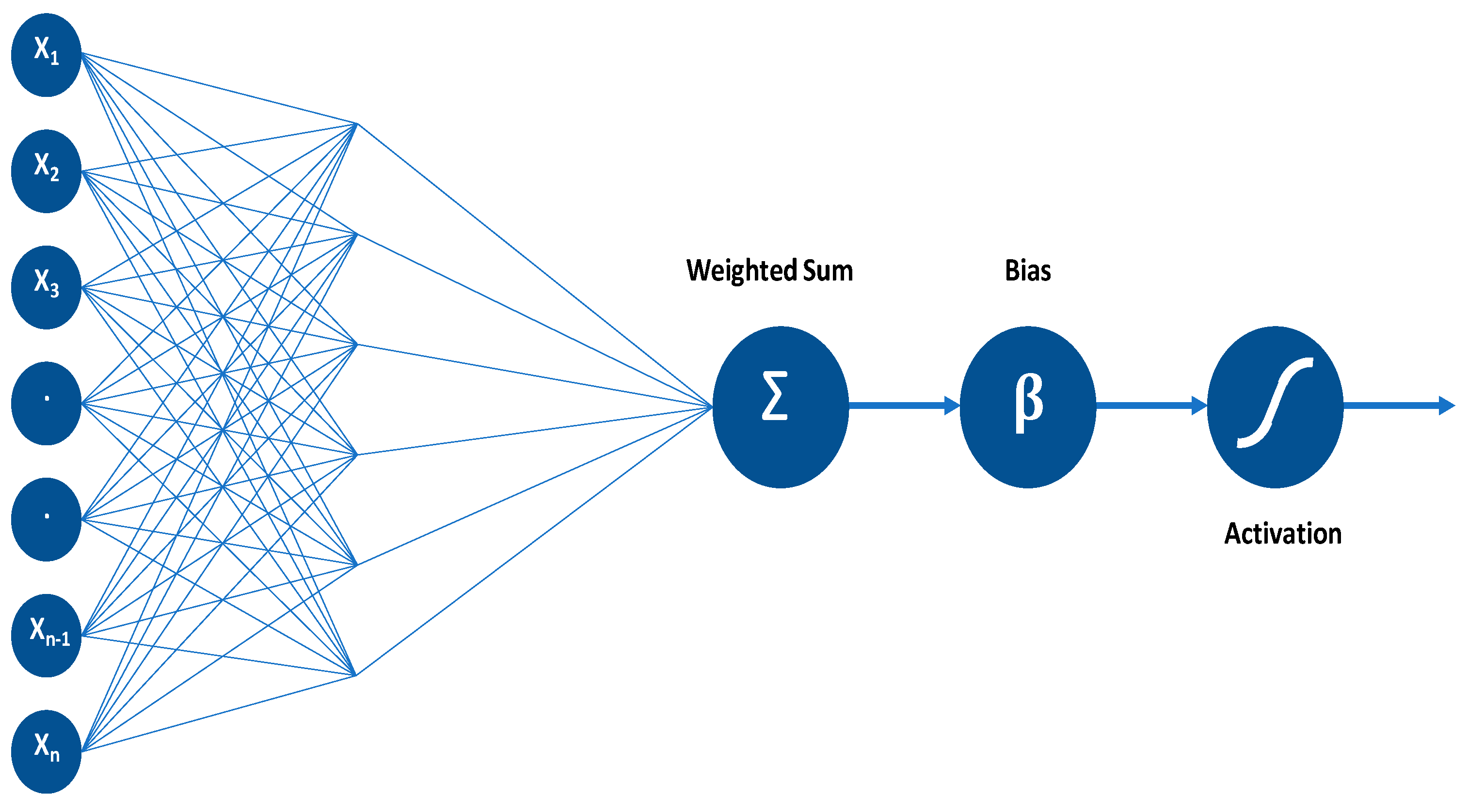
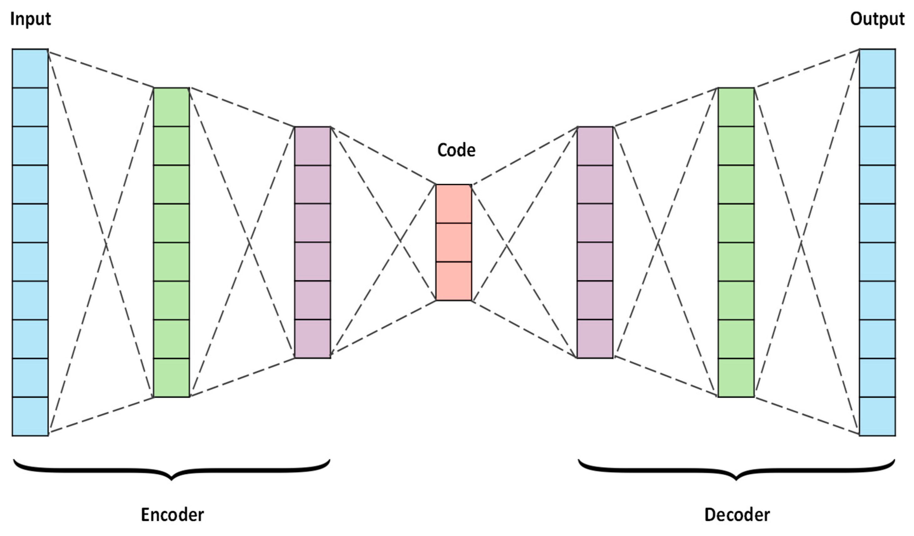
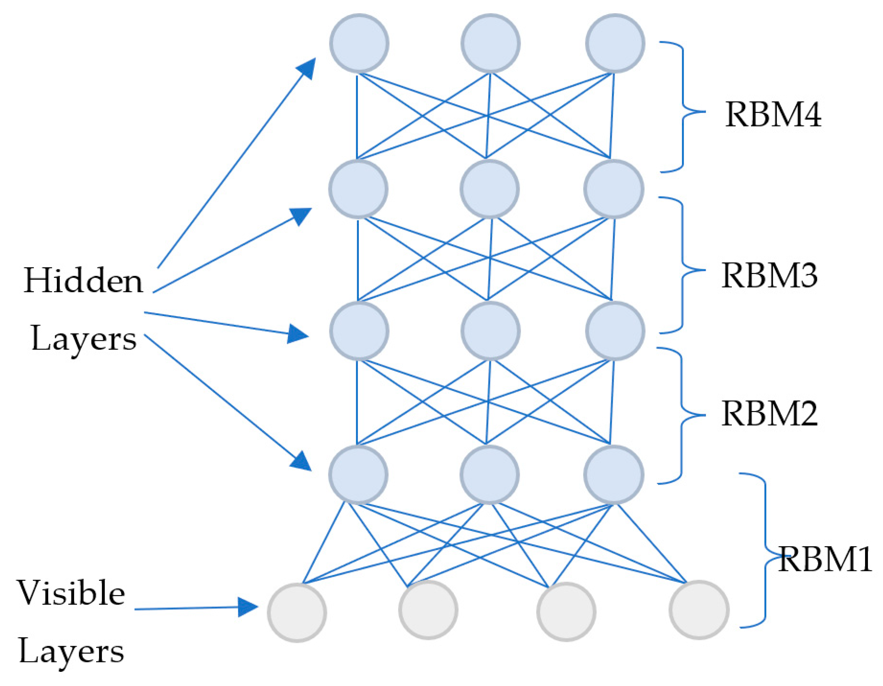
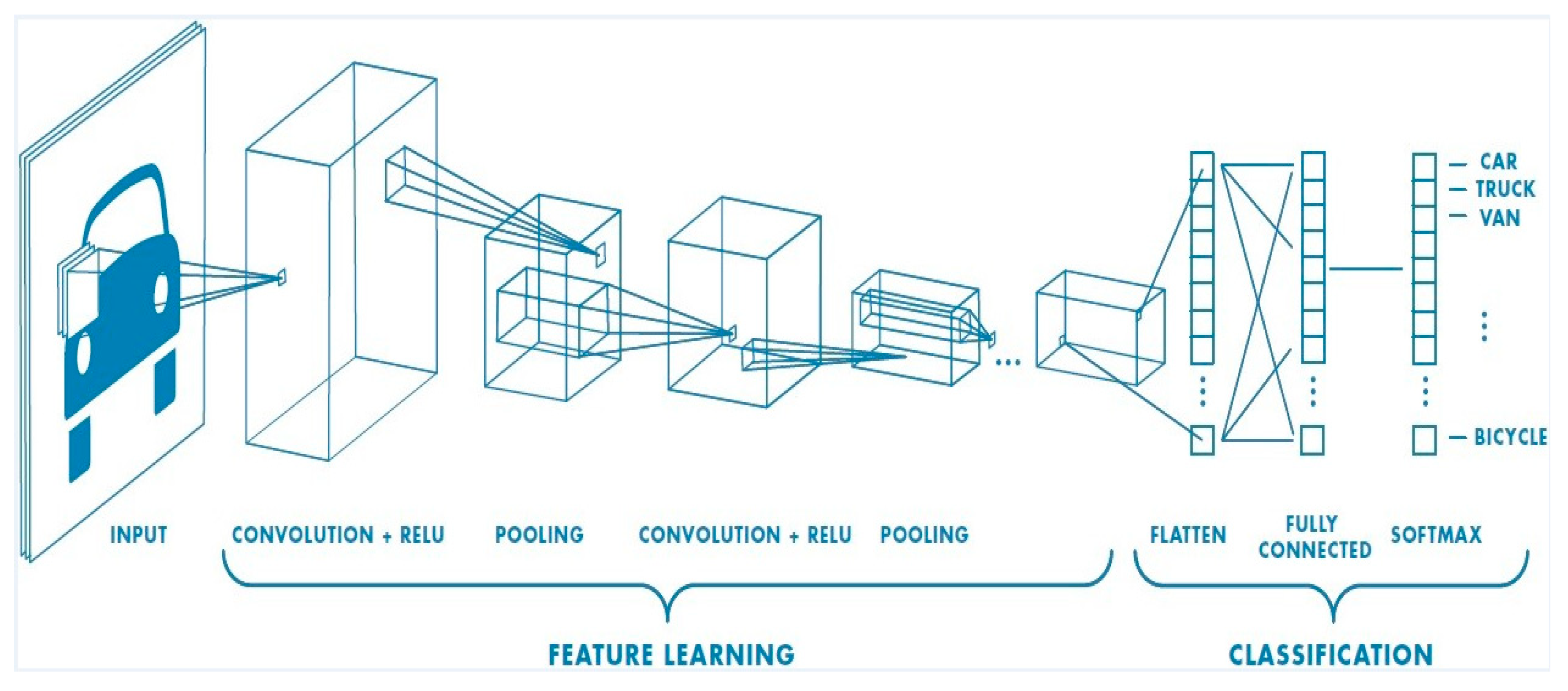
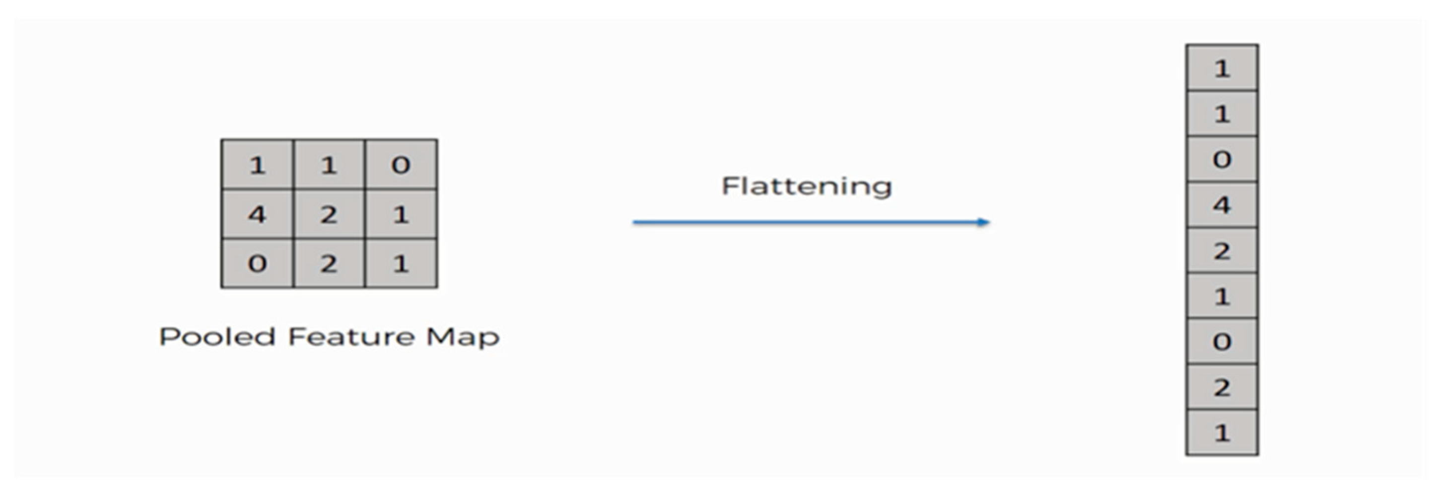
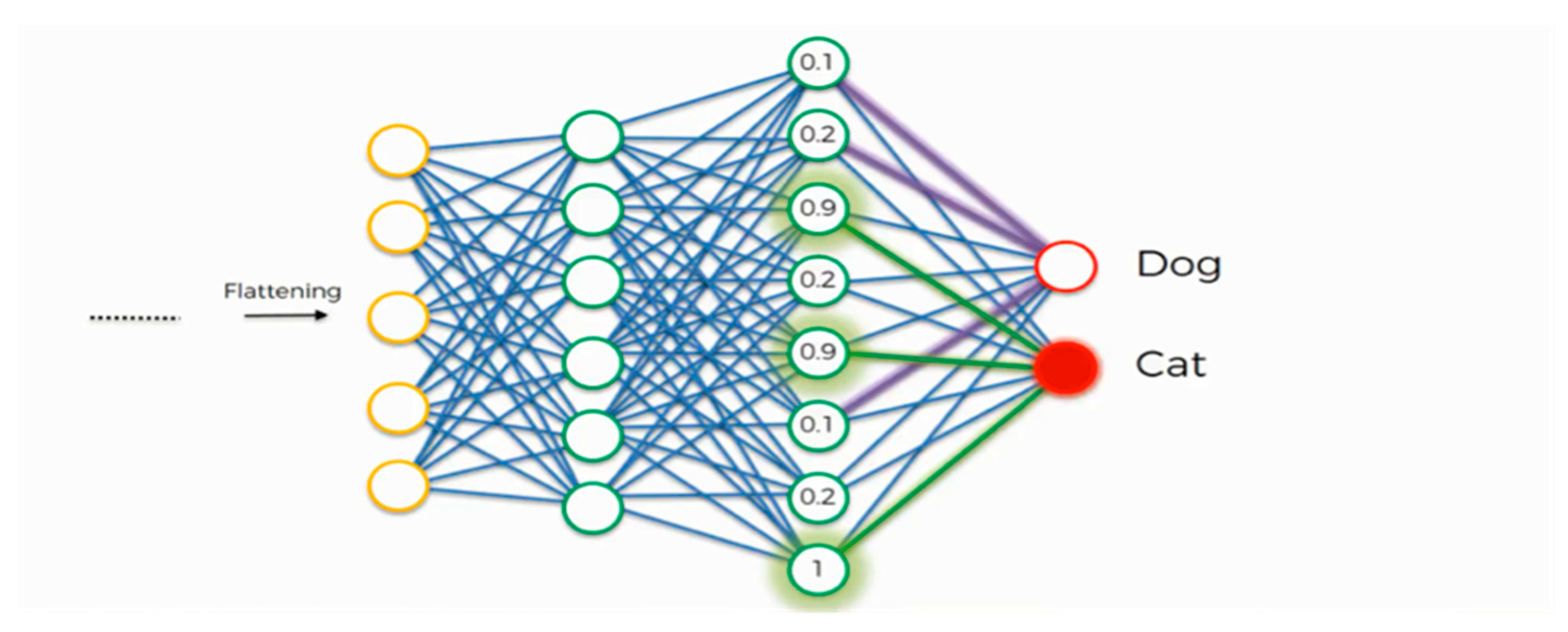
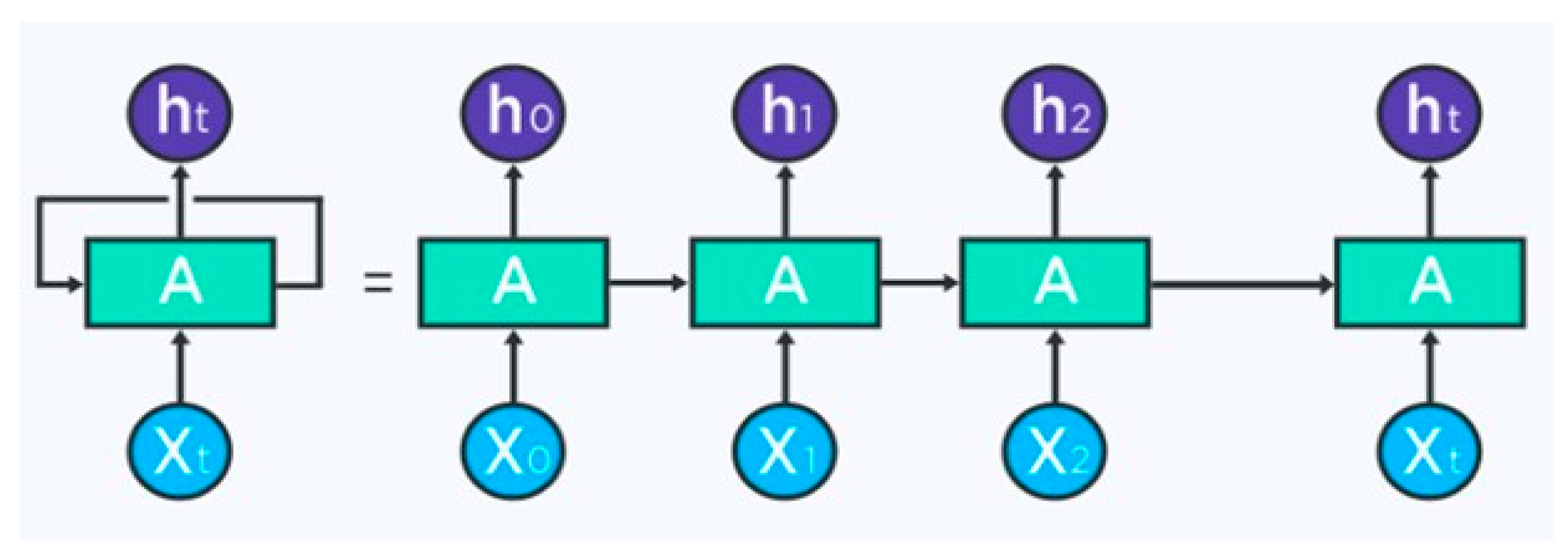
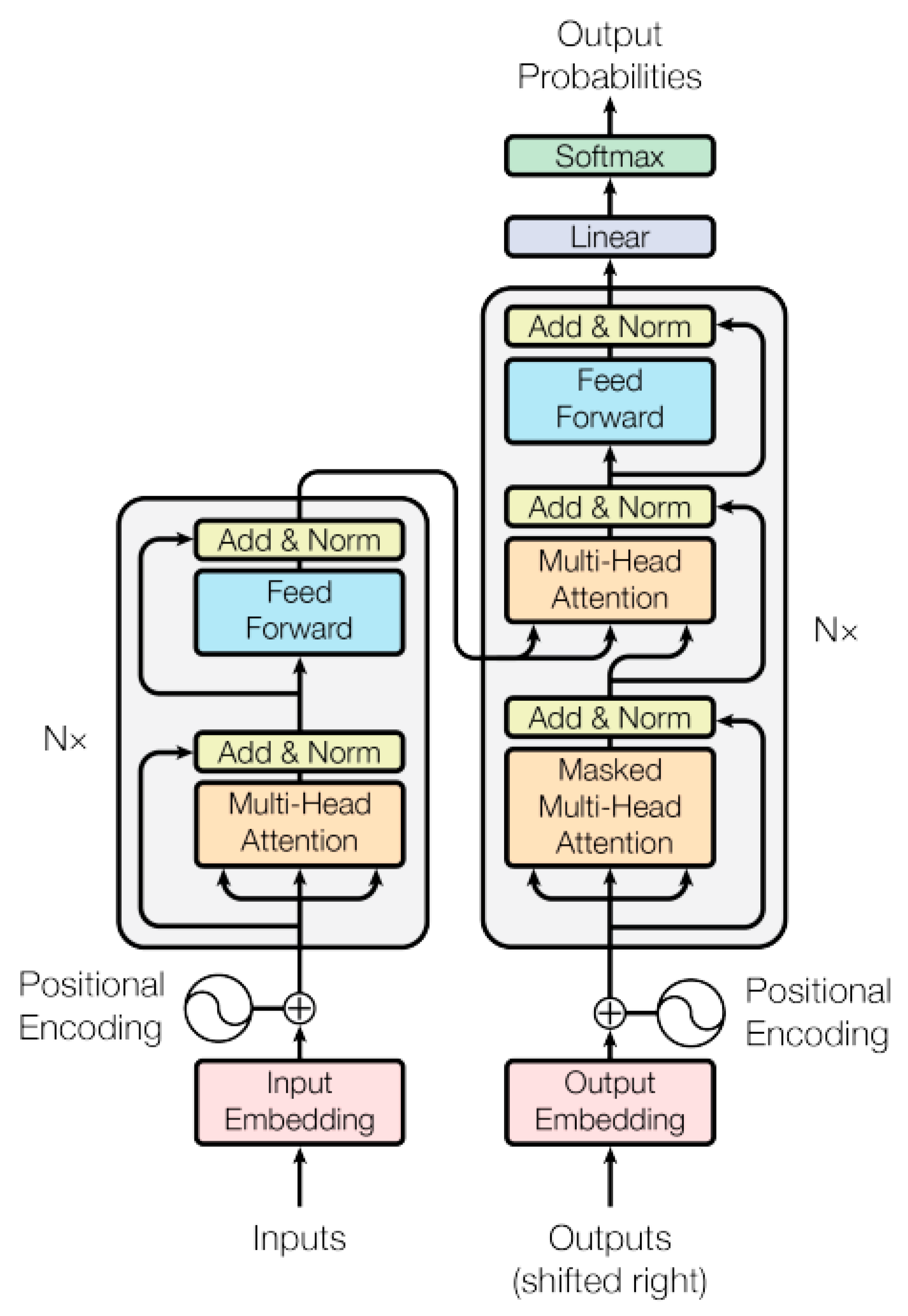