
Modular Stability Analysis of a Nonlinear Stochastic Fractional Volterra IDE


Abstract
:1. Introduction
2. Preliminaries
- (MI)
- for any iff ;
- (MII)
- for each , and with ;
- (MIII)
- for all and ;
- (MIV)
- is continuous.
3. Main Results
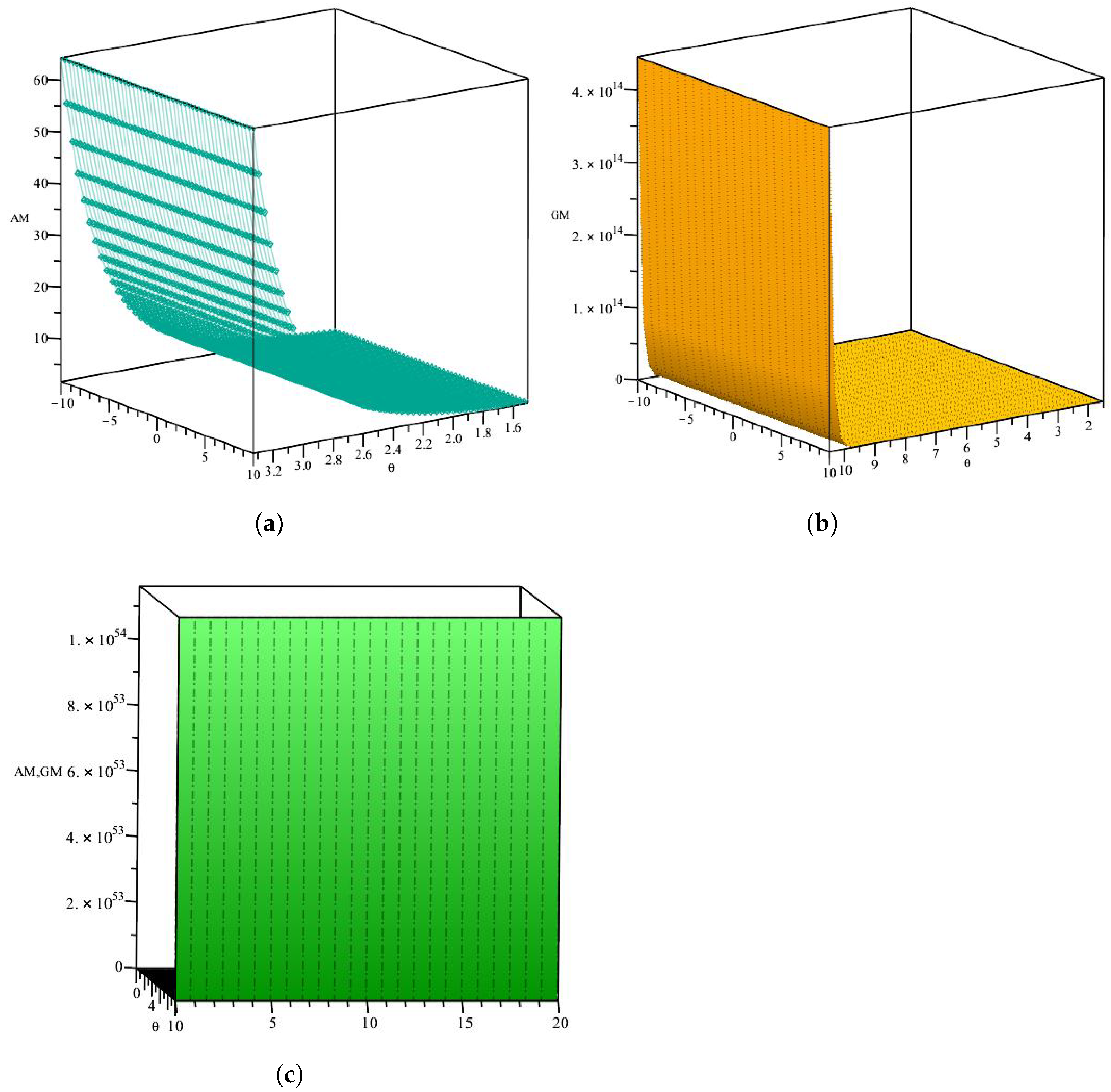
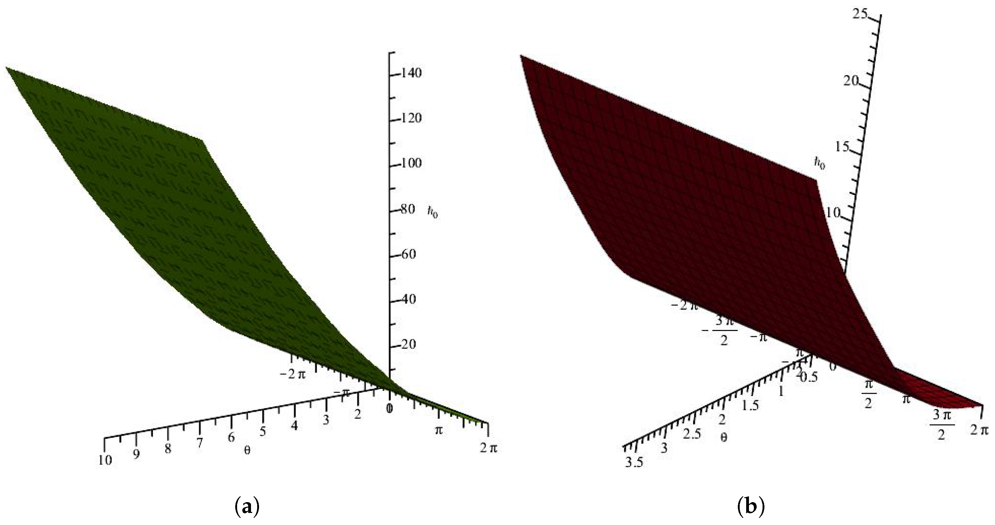
4. Example
5. Conclusions
Author Contributions
Funding
Data Availability Statement
Acknowledgments
Conflicts of Interest
References
- Ahmadi, N.; Vahidi, A.R.; Allahviranloo, T. An efficient approach based on radial basis functions for solving stochastic fractional differential equations. Math. Sci. 2017, 11, 13–118. [Google Scholar] [CrossRef] [Green Version]
- Raza, A.; Arif, M.S.; Rafiq, M.; Bibi, M.; Fayyaz, R. Numerical analysis of stochastic vector borne plant disease model. Comput. Mater. Contin. 2020, 63, 65–83. [Google Scholar]
- Nakano, H. Modular Semi-Ordered Spaces; Maruzen Co., Ltd.: Tokyo, Japan, 1950. [Google Scholar]
- Musielak, J.; Orlicz, W. On modular space. Stud. Math. 1959, 18, 49–65. [Google Scholar] [CrossRef]
- Krasnoselskii, M.A.; Rutickii, Y.B. Convex Functions and Orlicz Spaces; Noordhoff, G., Translator; Fizmatgiz: Moscow, Russia, 1961. (In Russian) [Google Scholar]
- Cădariu, L.; Radu, V. Fixed points and the stability of Jensen’s functional equation. JIPAM J. Inequal. Pure Appl. Math 2003, 4, 4. [Google Scholar]
- Diaz, J.B.; Margolis, B. A fixed point theorem of the alternative, for contractions on a generalized complete metric space. Bull. Amer. Math. Soc. 1968, 74, 305–309. [Google Scholar] [CrossRef] [Green Version]
- Sousa, J.V.C.; de Oliveira, E.C. On a new operator in fractional calculus and applications. J. Fixed Point Theory Appl. 2018, 20, 96. [Google Scholar] [CrossRef]
- Sousa, J.V.d.C.; de Oliveira, E.C. On the Φ-Hilfer fractional derivative. Commun. Nonlinear Sci. Numer. Simul. 2018, 60, 72–91. [Google Scholar] [CrossRef]
- Sevgin, S.; Sevli, H. Stability of a nonlinear Volterra integro-differential equation via a fixed point approach. J. Nonlinear Sci. Appl. 2016, 9, 200–207. [Google Scholar] [CrossRef] [Green Version]
- Eidinejad, Z.; Saadati, R.; Mesiar, R. Optimum Approximation for ς-Lie Homomorphisms and Jordan ς-Lie Homomorphisms in ς-Lie Algebras by Aggregation Control Functions. Mathematics 2022, 10, 1704. [Google Scholar] [CrossRef]
- Ahmed, N.; Wei, Z.; Baleanu, D.; Rafiq, M.; Rehman, M.A. Spatio-temporal numerical modeling of reaction-diffusion measles epidemic system. Chaos 2019, 29, 103101. [Google Scholar] [CrossRef]
- Namjoo, M.; Zibaei, S. A NSFD scheme for the solving fractional-order competitive prey-predator system. Thai J. Math. 2020, 18, 1933–1945. [Google Scholar]
- Namjoo, M.; Zeinadini, M.; Zibaei, S. Nonstandard finite-difference scheme to approximate the generalized Burgers-Fisher equation. Math. Methods Appl. Sci. 2018, 41, 8212–8228. [Google Scholar] [CrossRef]
- Zibaei, S.; Namjoo, M. A nonstandard finite difference scheme for solving fractional-order model of HIV-1 infection of CD4+ T-cells. IJMC 2015, 6, 169–184. [Google Scholar]
- Baleanu, D.; Zibaei, S.; Namjoo, M.; Jajarmi, A. A nonstandard finite difference scheme for the modeling and nonidentical synchronization of a novel fractional chaotic system. Adv. Differ. Equ. 2021, 2021, 308. [Google Scholar] [CrossRef]
- Macías-Díaz, J.E.; Raza, A.; Ahmed, N.; Rafiq, M. Analysis of a nonstandard computer method to simulate a nonlinear stochastic epidemiological model of coronavirus-like diseases. Comput. Methods Programs Biomed. 2021, 204, 106054. [Google Scholar] [CrossRef]
- Nauman, A.; Macías-Díaz, J.E.; Raza, A.; Baleanu, D.; Rafiq, M.; Iqbal, Z.; Ahmad, M.O. Design, Analysis and Comparison of a Nonstandard Computational Method for the Solution of a General Stochastic Fractional Epidemic Model. Axioms 2021, 11, 10. [Google Scholar]
- Noor, M.A.; Raza, A.; Arif, M.S.; Rafiq, M.; Nisar, K.S.; Khan, I.; Abdelwahab, S.F. Non-standard computational analysis of the stochastic COVID-19 pandemic model: An application of computational biology. Alex. Eng. J. 2022, 61, 619–630. [Google Scholar] [CrossRef]
- Win, Z.T.; Eissa, M.A.; Tian, B. Stochastic epidemic model for COVID-19 transmission under intervention strategies in China. Mathematics 2022, 10, 3119. [Google Scholar] [CrossRef]
- Yasin, M.W.; Iqbal, M.S.; Ahmed, N.; Akgül, A.; Raza, A.; Rafiq, M.; Riaz, M.B. Numerical scheme and stability analysis of stochastic Fitzhugh–Nagumo model. Results Phys. 2022, 32, 105023. [Google Scholar] [CrossRef]
- Shatanawi, W.; Raza, A.; Arif, M.S.; Abodayeh, K.; Rafiq, M.; Bibi, M. Design of nonstandard computational method for stochastic susceptible–infected–treated–recovered dynamics of coronavirus model. Adv. Differ. Equ. 2020, 2020, 505. [Google Scholar] [CrossRef]
- Raza, A.; Rafiq, M.; Ahmed, N.; Khan, I.; Nisar, K.S.; Iqbal, Z. A structure preserving numerical method for solution of stochastic epidemic model of smoking dynamics. Comput. Mater. Contin. 2020, 65, 263–278. [Google Scholar] [CrossRef]
- Shatanawi, W.; Raza, A.; Muhammad, S.A.; Abodayeh, K.; Rafiq, M.; Bibi, M. An effective numerical method for the solution of a stochastic coronavirus (2019-nCovid) pandemic model. Comput. Mater. Contin. 2021, 66, 1121–1137. [Google Scholar] [CrossRef]


Publisher’s Note: MDPI stays neutral with regard to jurisdictional claims in published maps and institutional affiliations. |
© 2022 by the authors. Licensee MDPI, Basel, Switzerland. This article is an open access article distributed under the terms and conditions of the Creative Commons Attribution (CC BY) license (https://creativecommons.org/licenses/by/4.0/).
Share and Cite
Ahadi, A.; Eidinejad, Z.; Saadati, R.; O’Regan, D. Modular Stability Analysis of a Nonlinear Stochastic Fractional Volterra IDE. Algorithms 2022, 15, 459. https://doi.org/10.3390/a15120459
Ahadi A, Eidinejad Z, Saadati R, O’Regan D. Modular Stability Analysis of a Nonlinear Stochastic Fractional Volterra IDE. Algorithms. 2022; 15(12):459. https://doi.org/10.3390/a15120459
Chicago/Turabian StyleAhadi, Azam, Zahra Eidinejad, Reza Saadati, and Donal O’Regan. 2022. "Modular Stability Analysis of a Nonlinear Stochastic Fractional Volterra IDE" Algorithms 15, no. 12: 459. https://doi.org/10.3390/a15120459