Personalized Federated Multi-Task Learning over Wireless Fading Channels

Abstract

Multi-task learning (MTL) is a paradigm to learn multiple tasks simultaneously by utilizing a shared network, in which a distinct header network is further tailored for fine-tuning for each distinct task. Personalized federated learning (PFL) can be achieved through MTL in the context of federated learning (FL) where tasks are distributed across clients, referred to as personalized federated MTL (PF-MTL). Statistical heterogeneity caused by differences in the task complexities across clients and the non-identically independently distributed (non-i.i.d.) characteristics of local datasets degrades the system performance. To overcome this degradation, we propose FedGradNorm, a distributed dynamic weighting algorithm that balances learning speeds across tasks by normalizing the corresponding gradient norms in PF-MTL. We prove an exponential convergence rate for FedGradNorm. Further, we propose HOTA-FedGradNorm by utilizing over-the-air aggregation (OTA) with FedGradNorm in a hierarchical FL (HFL) setting. HOTA-FedGradNorm is designed to have efficient communication between the parameter server (PS) and clients in the power- and bandwidth-limited regime. We conduct experiments with both FedGradNorm and HOTA-FedGradNorm using MT facial landmark (MTFL) and wireless communication system (RadComDynamic) datasets. The results indicate that both frameworks are capable of achieving a faster training performance compared to equal-weighting strategies. In addition, FedGradNorm and HOTA-FedGradNorm compensate for imbalanced datasets across clients and adverse channel effects.

1. Introduction

Multi-tasking (MTL) is a powerful technique for learning several related tasks simultaneously [1,2]. MTL improves the overall system performance, the training speed, and data efficiency, by leveraging the synergy among multiple related tasks. Each task in MTL setting has a single common encoder network to map the raw data into a lower dimensional shared representation space, in addition to a unique client-specific header network to infer task related prediction values from the shared representation. MTL is particularly suitable for distributed learning settings where no single entity has all the data and labels for all of the multiple different tasks.

Federated learning (FL) [3] is a distributed learning paradigm in which many clients train a shared model with the assistance of a central unit called parameter server (PS) by keeping their data private and decentralized. Statistical heterogeneity becomes a major challenge for FL as the size of the distributed setting, namely the number of clients or the number of tasks in a FL setting, increases. This is caused by different task complexities and non-i.i.d. data distribution among clients. Statistical heterogeneity due to non-i.i.d. data distribution degrades the system performance [4,5]. Further, synergy between the tasks may not always be positive, referred to as a negative transference, again degrading the performance [6].

Personalized federated learning (PFL) is introduced to deal with statistical heterogeneity, where the centralized server and clients learn a shared representation together, while each client trains its own client-specific header network further, referred to as personalization. PFL has the capability of learning user-specific models better while also capturing the distilled common knowledge from other clients [7,8,9]. As a result, PFL reduces the statistical heterogeneity among clients. Several PFL approaches have been proposed, where different local models are used to fit user-specific data, but also capture the common knowledge distilled from data of other devices for this purpose [7,8,9,10,11,12,13,14,15]. Hanzely et al. [16] provides a unified model framework to prove multiple kinds of PFL methods. In this paper, we consider MTL in a FL setting, enhanced with personalization, namely, personalized federated multi-task learning (PF-MTL).

PFL works that are closely related to our work are federated representation learning FedRep [7] and federated learning with personalization layers FedPer [8]. These works use a shared encoder with a unique task-specific header to enhance personalization in a FL setup. FedRep and FedPer aggregate the common encoder parameters by equal weighting. Our goal in this paper is to perform weighted gradient aggregation at the PS dynamically according to gradient updates coming from clients to overcome statistical heterogeneity.

Several approaches involve setting the weights of tasks manually at the beginning of training [17,18]. Task weights can also be set in an adaptive manner for each iteration. GradNorm is a dynamic weighting approach in MTL that normalizes gradient norms by scaling the task loss functions to regulate learning speeds and fairness across tasks [19]. GradNorm is proposed for a centralized learning setting. In our work, we introduce FedGradNorm framework [20], where dynamic weighting is incorporated in PFL setting by considering some aspects of [7,8,19] together. We provide a theoretical convergence proof for FedGradNorm, while FedPer [8] and GradNorm [19] do not provide a convergence proof, and FedRep [7] provides a convergence proof only for the linear learning model setting.

We investigate how the FedGradNorm framework is affected by the characteristics of the wireless fading communication channel between clients and the PS. There are different channel conditions since clients are geographically spread out. In addition to the wireless channel effects, the communication is performed over bandwidth- and power-limited regime, which brings concerns about communication costs. We utilize over-the-air (OTA) aggregation to perform efficient aggregation over a shared wireless channel to support the clients on the same bandwidth by utilizing the additive nature of wireless multiple access channel (MAC) [21,22]. In practice, when the OTA mechanism is utilized, the gradients are superposed, and it is not possible for the PS to receive individual gradients of the clients. However, the PS needs individual gradients from the clients to perform dynamic weighting. To address this issue, we modify FedGradNorm with OTA in a hierarchical structure, which is called hierarchical over-the-air FedGradNorm, HOTA-FedGradNorm [23]. Hierarchical federated learning (HFL) establishes clusters of clients around intermediate servers (IS). ISs communicate with the PS instead of clients directly communicating with the PS. Some aspects of HFL have been studied in the literature, such as, latency and power analysis [24,25], and resource allocation [26,27]. These works demonstrate the advantage of the proximity of ISs to the clients in terms of resource consumption of clients. In addition to these advantages, we utilize hierarchical structure since it provides an efficient way of combining FedGradNorm with OTA over the wireless fading channel.

The main contributions of our paper can be summarized as:

• We propose the FedGradNorm algorithm. The proposed algorithm takes advantage of the GradNorm [19] dynamic weighting strategy in a PFL setup for achieving a more effective and fair learning performance when the clients have a diverse set of tasks to perform.
• We propose HOTA-FedGradNorm. The proposed algorithm takes into account the characteristics of the communication channel by defining a hierarchical structure for the PFL setting.
• We provide the convergence analysis for adaptive weighting strategy for MTL in PFL setting. Existing works either do not provide convergence analysis or do it in special cases. We demonstrate that FedGradNorm has an exponential convergence rate.
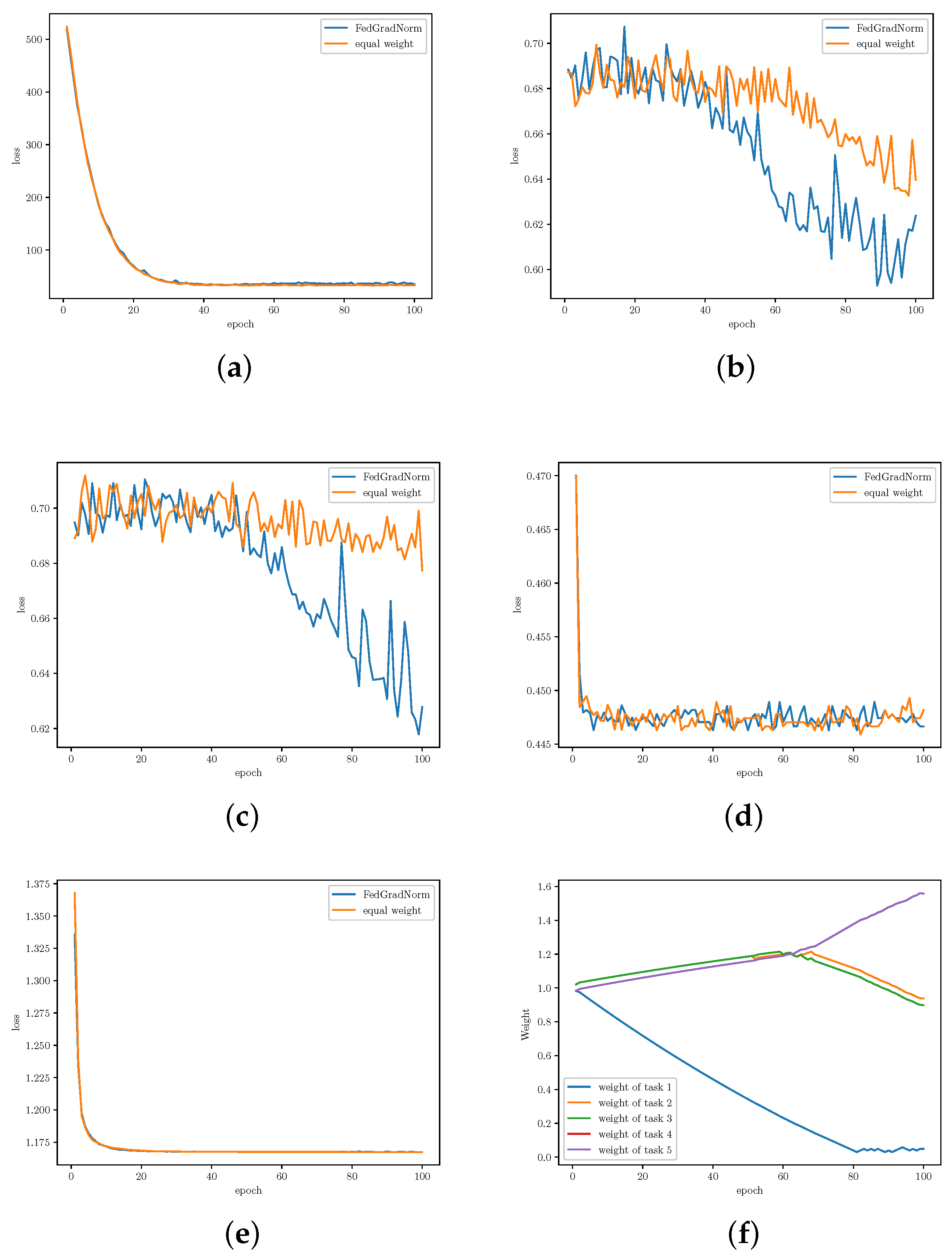
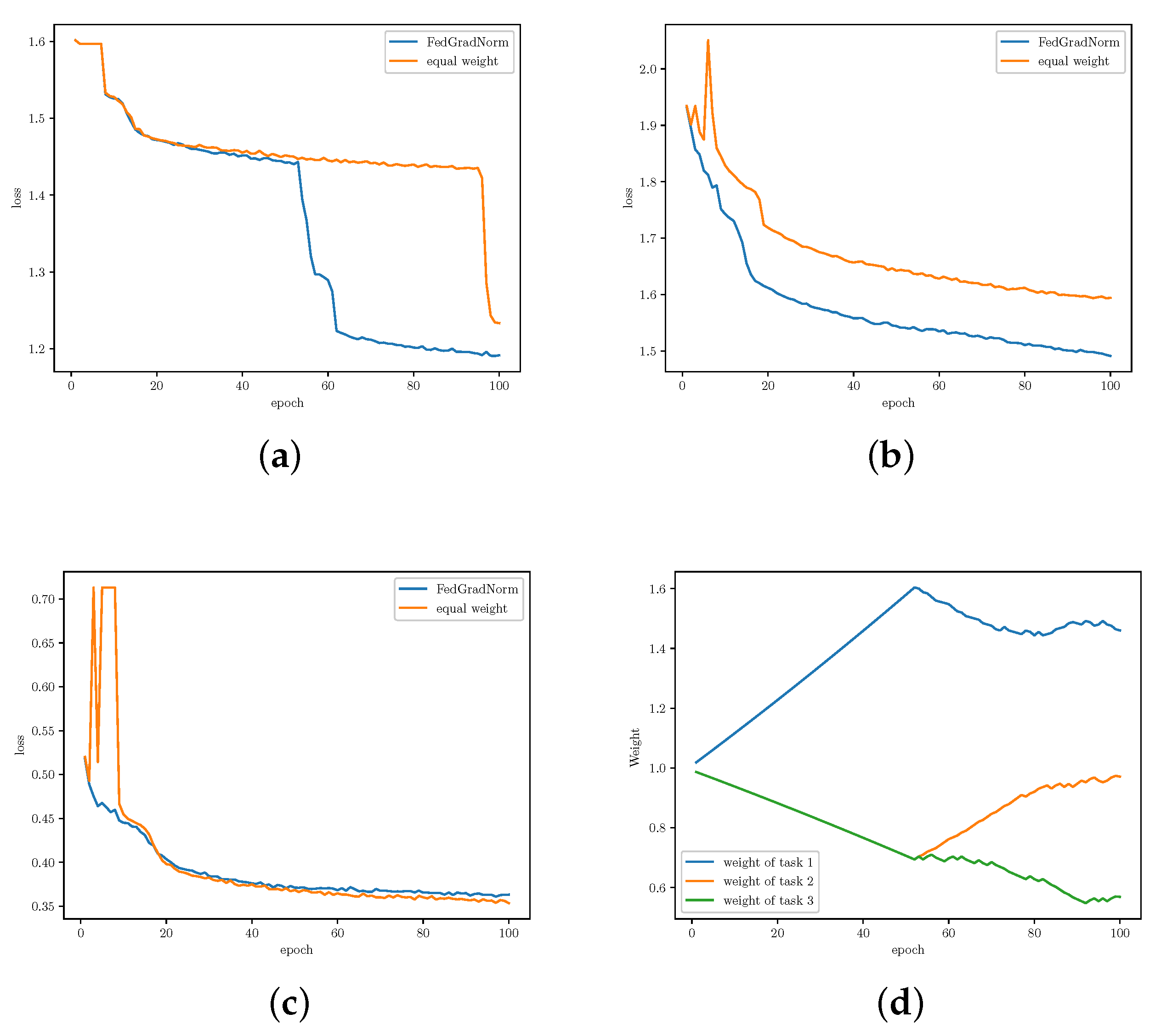
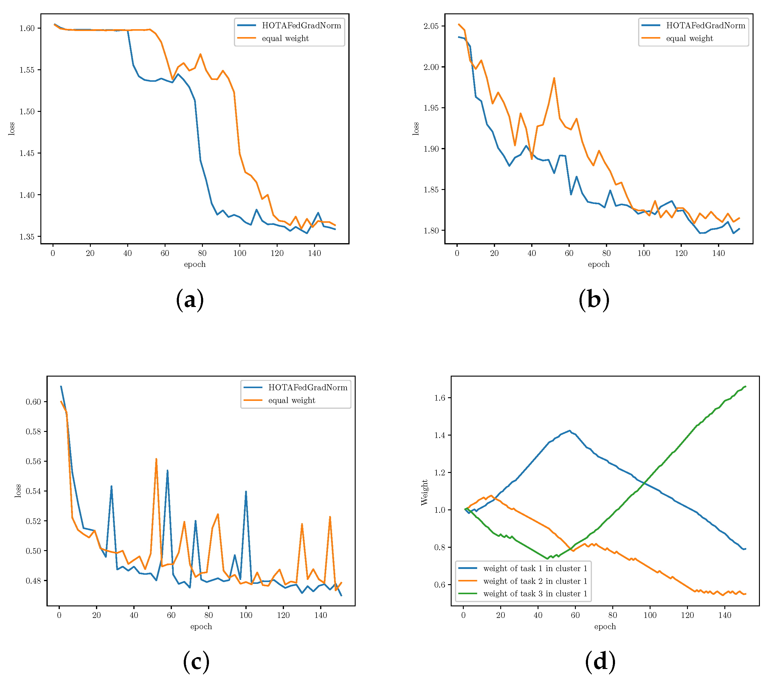
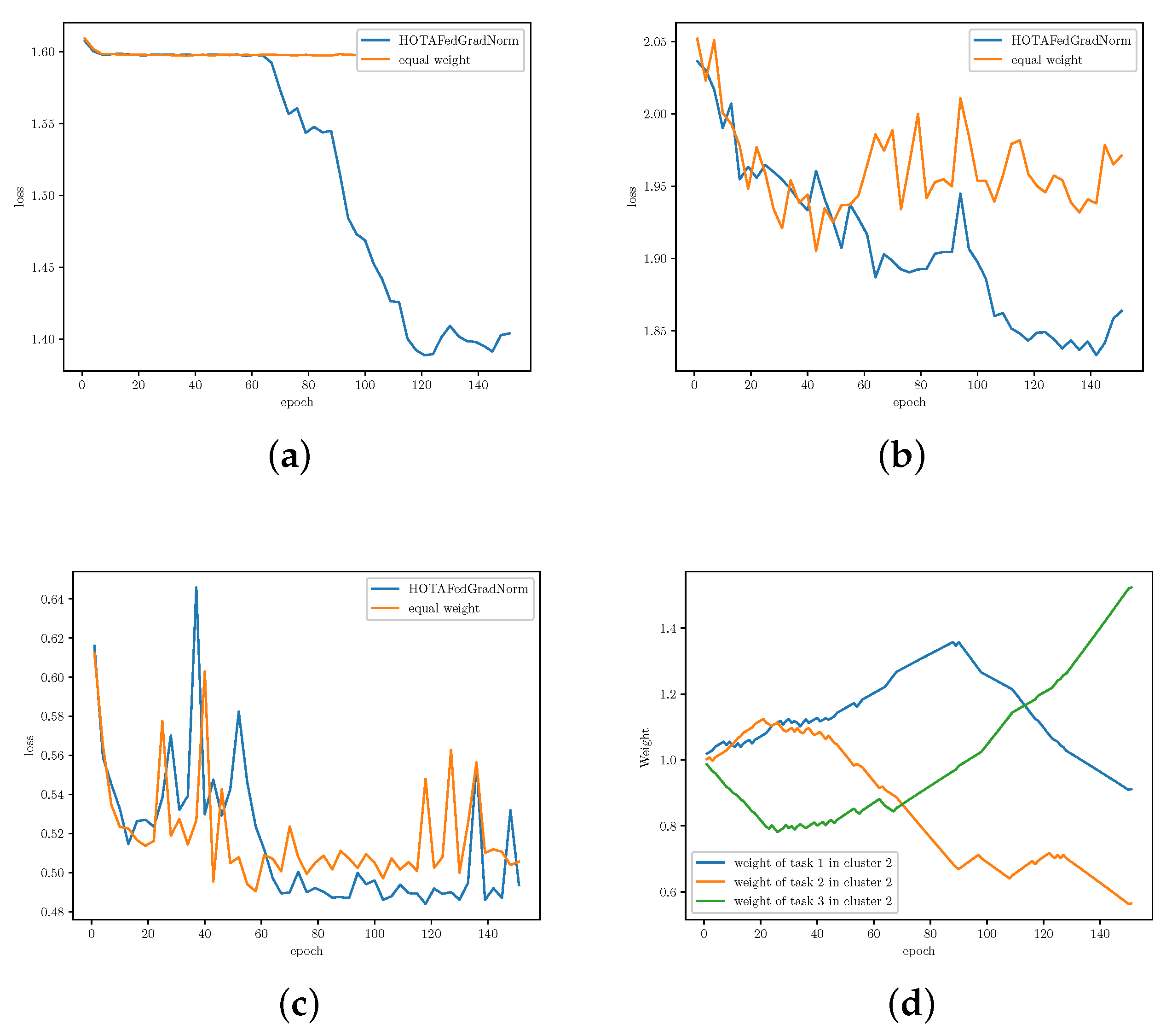
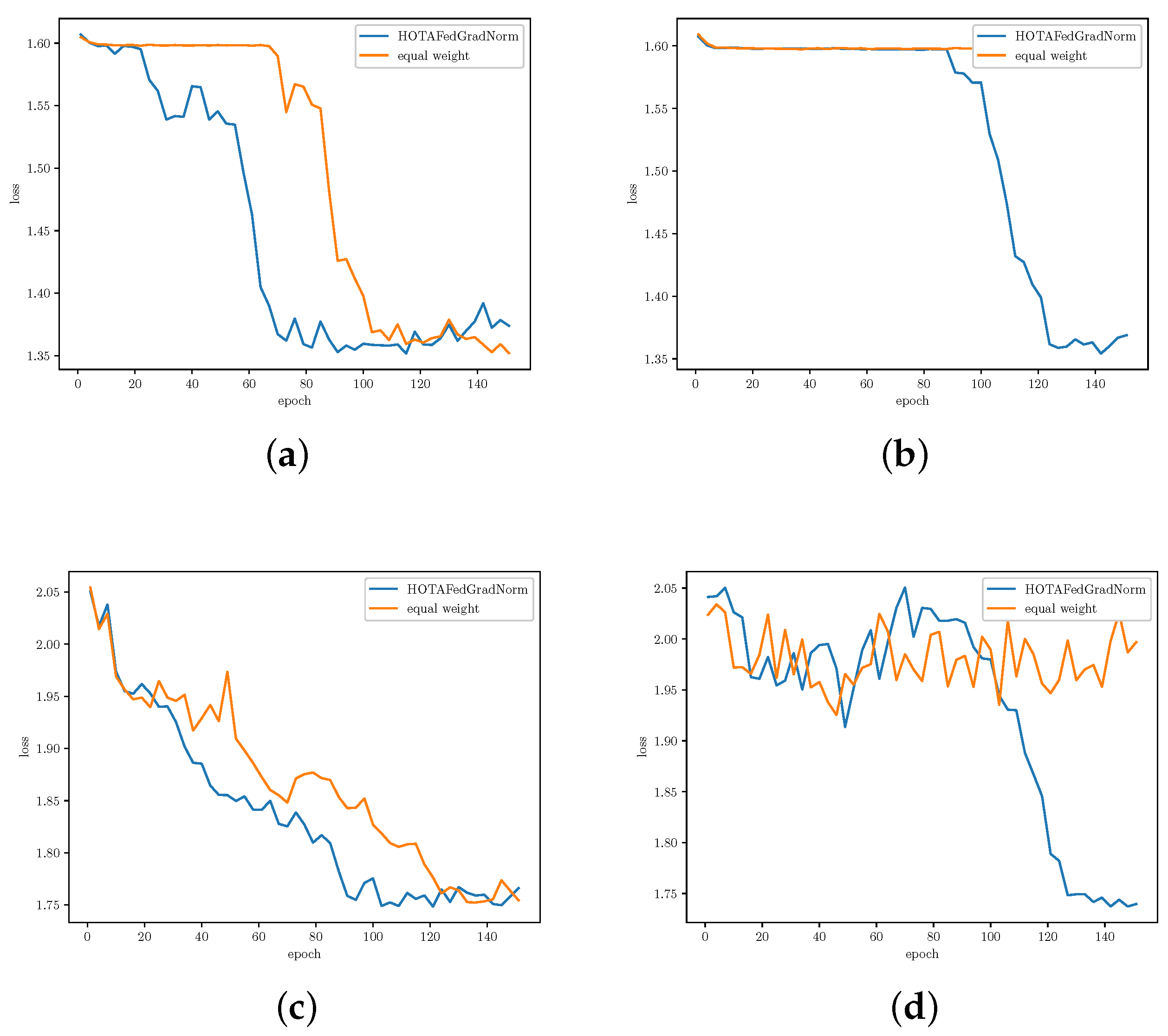
• We conduct several experiments on our framework using Multi-Task Facial Landmark (MTFL) dataset [28], and RadComDynamic dataset on the wireless communication domain [29]. We investigate the changes in task loss during training to compare the learning speed and fairness of FedGradNorm with a similar PFL setting which uses equal weighting technique, namely FedRep. Experimental results exhibit a better and faster learning performance for FedGradNorm than FedRep. In addition, we demonstrate that HOTA-FedGradNorm results in faster training over the wireless fading channel compared to algorithms with naive static equal weighting strategies since dynamic weight selection process takes the channel conditions into account.

2. System Model and Problem Formulation

2.1. Federated Learning (FL)

FL [3] is a distributed machine learning approach that enables training on decentralized data in devices such as smart phones, IoT devices, and so on. FL can be described as an approach that brings the training model to the data, instead of bringing data to the training model [30]. In FL, edge devices collaboratively learn a shared model under the orchestration of a PS without sharing their training data.

The generic form of FL with N clients is

$$\begin{array}{c}\hfill \underset{\omega }{min}\left\{F(\omega )\triangleq \frac{1}{N}\sum _{i=1}^N{p}^{(i)}{F}^{(i)}(\omega )\right\}\end{array}$$

(1)

where $p^{(i)}$ is the loss weight for client i such that ${\sum }_{i=1}^N{p}^{(i)}=N$, and $F^{(i)}$ is the local loss function for client i.

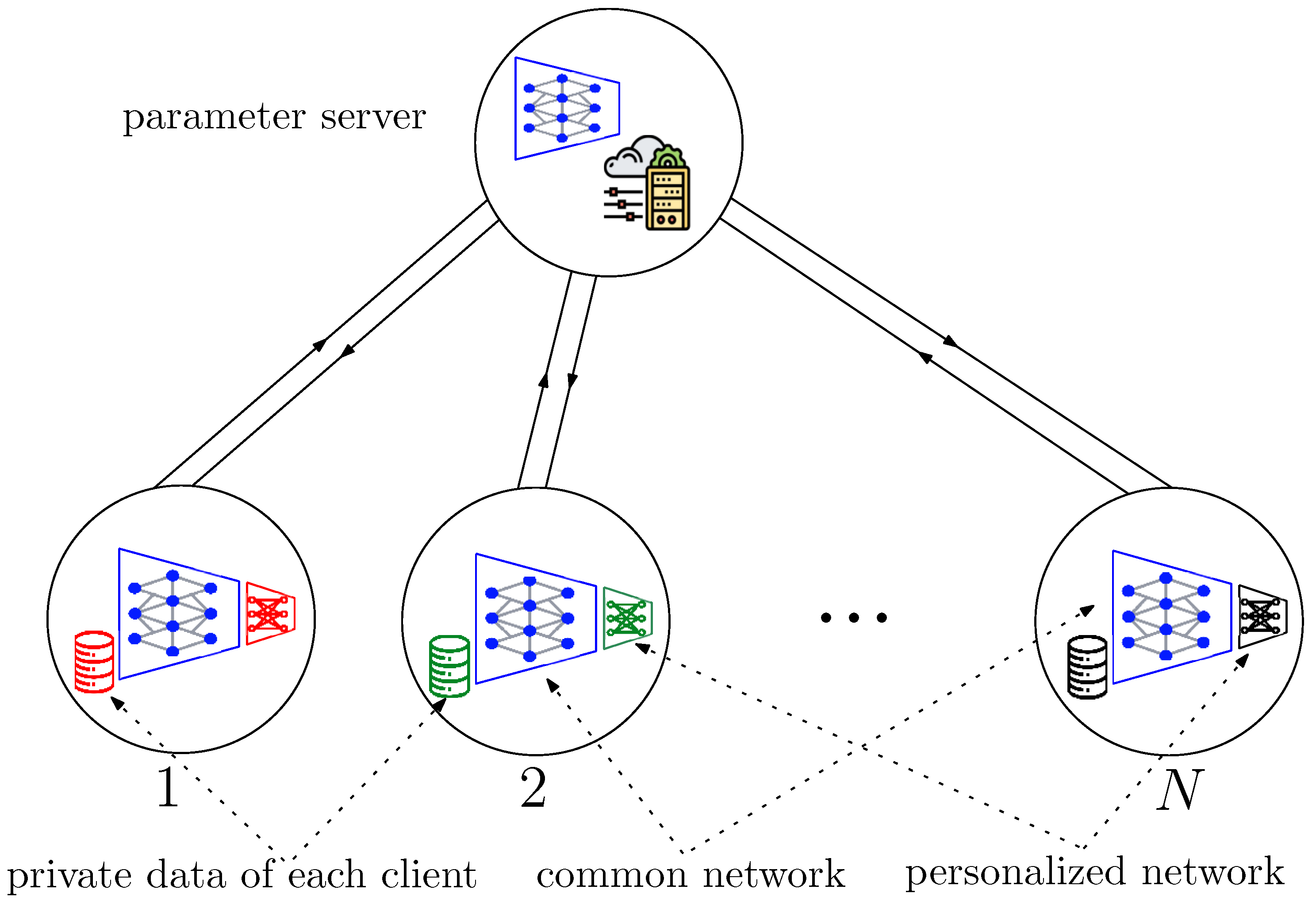
2.2. Personalized Federated Multi-Task Learning (PF-MTL)

We consider a PFL setting with N clients, in which client i has its own local dataset $D_i={\{({\mathbf{x}}_j^{(i)},y_j^{(i)})\}}_{j=1}^{n_i}$ where $n_i$ is the size of the local dataset, and $T_i$ is the task of client i, $i\in \left[N\right]$. The system model consists of a global representation network $q_{\omega }:{\mathbb{R}}^d\to {\mathbb{R}}^{d^{\prime }}$ which is a function parameterized by $\omega \in \mathcal{W}$ and maps data points to a lower space of size $d^{\prime }$. All clients share the same global representation network which is synchronized across clients with global aggregation. Client-specific heads $q_{h^{(i)}}:{\mathbb{R}}^{d^{\prime }}\to \mathcal{Y}$ are functions parameterized by $h^{(i)}\in \mathcal{H}$ for all clients $i\in \left[N\right]$ and map from the low dimensional representation space to the label space $\mathcal{Y}$. The system model is shown in Figure 1. Then, the local model for the ith client is the composition of the ith client’s global representation model $q_{\omega }$ and the personalized model $q_{h^{(i)}}$,

$$\begin{array}{c}\hfill q_i(·)=(q_{h^{(i)}}\circ q_{\omega })(·)\end{array}$$

(2)

The local loss for the ith client is represented as

$$\begin{array}{c}\hfill F^{(i)}(h^{(i)},\omega )=F^{(i)}(q_i(·))=F^{(i)}((q_{h^{(i)}}\circ q_{\omega })(·))\end{array}$$

(3)

Through alternating minimization, the clients and the centralized server aim to learn a set of global parameters $\omega$ together, while each client i learns its own set of client-specific parameters $h^{(i)}$ locally. Specifically, client i performs ${\tau }_h$ local gradient based updates to optimize $h^{(i)}$, $i\in \left[N\right]$, while the global network parameters at client i, i.e., ${\omega }^{(i)}$, are frozen. Thereafter, client i performs ${\tau }_{\omega }$ local updates to optimize the global shared network parameters, while the parameters corresponding to the client-specific head are frozen. Then, the global shared network parameters ${\{{\omega }^{(i)}\}}_{i=1}^N$ are aggregated at the PS to obtain a common $\omega$. Thus, the problem is   

$$\begin{array}{c}\hfill \underset{\omega \in \mathcal{W}}{min}\frac{1}{N}\sum _{i=1}^N{p}^{(i)}\underset{h^{(i)}\in \mathcal{H}}{min}{F}^{(i)}(h^{(i)},\omega )\end{array}$$

(4)

FedRep [7] investigates this framework with $p^{(i)}=1$, $i\in \left[N\right]$.

2.3. PF-MTL as Bilevel Optimization Problem

The optimization problem in (4) can be rewritten as (5) because $F^{(i)}(h^{(i)},\omega )$ relies on only $h^{(i)}$ and $\omega$ for all $i\in \left[N\right]$, and $h^{(i)}$ are independent of each other

$$\begin{array}{c}\hfill \underset{\omega \in \mathcal{W}}{min}\underset{{\{h^{(i)}\in \mathcal{H}\}}_{i=1}^N}{min}\frac{1}{N}\sum _{i=1}^N{p}^{(i)}{F}^{(i)}(h^{(i)},\omega )\end{array}$$

(5)

Equivalently, we have

$$\begin{array}{c}\hfill \underset{\omega \in \mathcal{W},{\{h^{(i)}\in \mathcal{H}\}}_{i=1}^N}{min}\frac{1}{N}\sum _{i=1}^N{p}^{(i)}{F}^{(i)}(h^{(i)},\omega )\end{array}$$

(6)

Note that $p^{(i)}$ values in (6) are obtained from our proposed FedGradNorm algorithm which will be derived later as a consequence of another optimization problem. As a result, the problem can be expressed as a bilevel optimization problem, which is an optimization problem containing another optimization problem as a constraint

$$\begin{array}{cc}\hfill \underset{x_u\in X_u,x_l\in X_l}{min}& F(x_u,x_l)\hfill \\ \hfill \mathrm{s}.\mathrm{t}.& x_l=\underset{x_l\in X_l}{arg\; min}\{g(x_u,x_l),\mathrm{s}.\mathrm{t}.c_j(x_u,x_l)\le 0,j=1,\dots ,J\}\hfill \\ \hfill & C_m(x_u,x_l)\le 0,m=1,\dots ,M\hfill \end{array}$$

(7)

where $F(x_u,x_l)$ represents the upper-level objective function and $g(x_u,x_l)$ represents the lower-level objective function. $\{c_j(x_u,x_l)\le 0,j=1,\dots ,J\}$ are the constraints for the lower-level optimization problem while $\{C_m(x_u,x_l)\le 0,m=1,\dots ,M\}$ and the lower-level optimization problem itself are the constraints for the upper-level optimization problem.

Multiple algorithms have been developed to solve bilevel optimization problems in the literature [31]. Different reformulations of the bilevel optimization problem have been made by utilizing the optimality conditions of the lower-level optimization problem to formulate the bilevel optimization problem as a single-level constraint problem [32,33,34]. In addition, there are recently developed gradient-based bilevel optimization algorithms [35,36,37,38,39,40]. Our algorithm is based on iterative differentiation (ITD), as explained in Algorithm 1.

Algorithm 1 Iterative differentiation (ITD) algorithm.

Input: K, D, step sizes $\alpha$, $\beta$, initialization $x_u(0)$, $x_l(0)$. fork = 0, 1, 2, …, K do   Set $x_l^0(k)$ = $x_l^D(k-1)$ if $k>0$ otherwise $x_l(0)$.   for t = 1, …, D do     Update $x_l^t(k)=x_l^{t-1}(k)-\alpha {\nabla }_{x_l}g(x_u(k),x_l^{t-1}(k))$   Compute ${\widehat{\nabla }}_{x_u}F(x_u(k),x_l^D(k))=\frac{\partial F(x_u(k),x_l^D(k))}{\partial x_u}$   Update $x_u(k+1)=x_u(k)-\beta {\widehat{\nabla }}_{x_u}F(x_u(k),x_l^D(k))$

Updates to the upper-level optimization take place in the outer loop, while updates to the lower-level optimization are performed in the inner loop.

For our problem, $x_u$ and $x_l$ correspond to $\left({\{h^{(i)}\}}_{i=1}^N,\omega \right)$, ${\{p^{(i)}\}}_{i=1}^N$, respectively. Additionally, $x_u(k)$ and $x_l(k)$ are denoted as $\left({\{h^{(i)}\}}_{i=1}^N,{\omega }_k\right)$, ${\{p_k^{(i)}\}}_{i=1}^N$ to represent the outer loop iteration index in Algorithm 1 for the rest of the paper. Furthermore, i in $p_k^i$ represents the inner loop iteration index, while i in $p_k^{(i)}$ represents the client index. Then, the bilevel optimization problem in our case can be written as

$$\begin{array}{cc}\hfill \underset{\omega ,{\{h^{(i)}\}}_{i=1}^N,{\{p^{(i)}\}}_{i=1}^N}{min}& F({\{h^{(i)}\}}_{i=1}^N,\omega ,{\{p^{(i)}\}}_{i=1}^N)\hfill \\ \hfill \mathrm{s}.\mathrm{t}.& {\{p^{(i)}\}}_{i=1}^N\in \underset{{\{p^{(i)}\}}_{i=1}^N\in {\mathbb{R}}^N}{arg\; min}{F}_{grad}\hfill \end{array}$$

(8)

The objective function is a weighted sum of local loss functions, $F=\frac{1}{N}{\sum }_{i=1}^N{p}^{(i)}{F}^{(i)}(h^{(i)},\omega )$, and $F_{grad}$ is the auxiliary loss function defined by the FedGradNorm algorithm in the next section.

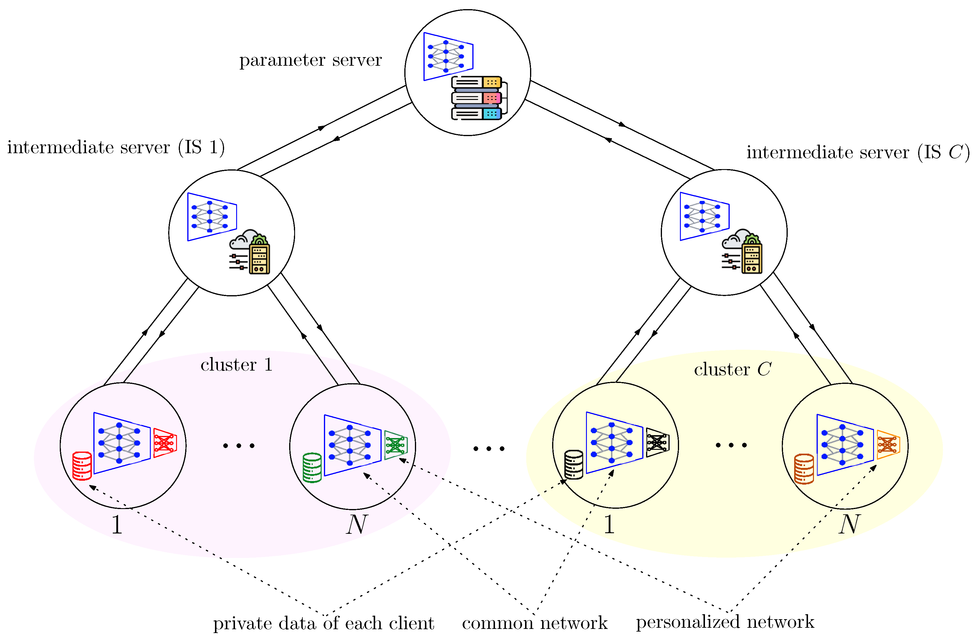
2.4. Hierarchical Federated Learning (HFL) for Wireless Fading Channels

The characteristics of the communication channel should be considered in PF-MTL, since clients can be distributed in a large geographic area in an FL framework [41,42]. The PS can be far away from the clients, and the communication between the PS and the clients can be noisy and subject to channel effects. Then, PF-MTL can be constructed in hierarchical setting by creating clusters of clients around IS to communicate with the PS instead of the direct communication of clients with the PS. Further, the communication can be performed over a shared wireless channel, where the transmission power and the bandwidth are constrained. Thus, we employ over-the-air aggregation (OTA) to address these issues [21,22].

The generic HFL problem shown in Figure 2, with C clusters each containing an IS and N clients, can be formulated as

$$\begin{array}{c}\hfill \underset{\omega }{min}\left\{F(\omega )\triangleq \frac{1}{CN}\sum _{l=1}^C\sum _{i=1}^N{p}^{(l,i)}{F}^{(l,i)}(\omega )\right\}\end{array}$$

(9)

where $p^{(l,i)}$ is the loss weight for client i in cluster l such that ${\sum }_{i=1}^N{p}^{(l,i)}=N$, $l\in \left[C\right]$, and $F^{(l,i)}(·)$ is the local loss function for client i in cluster l.

We consider a PFL setting of N clients within each cluster, in which client i of cluster l has its own local dataset $D_{l,i}={\{({\mathbf{x}}_j^{(l,i)},y_j^{(l,i)})\}}_{j=1}^{n_{l,i}}$ where $n_{l,i}$ is the size of the local dataset. Within cluster l, $T_{l,i}$ denotes the task of client i, $i\in \left[N\right]$, and $l\in \left[C\right]$. $T_{l,i}$ is assigned from the task set $\mathcal{T}=\{T_1,T_2,\dots ,T_N\}$ such that $T_{l,i}\ne T_{l,i^{\prime }}$, for $i\ne i^{\prime }$ and for any $l\in \left[C\right]$. Real-life scenarios might involve the same or very similar tasks for clients in a cluster. We assume that tasks are different due to the lack of prior information about it.

We assume that clients in a cluster have error-free and high-speed connections to corresponding IS over local area networks (LANs). In addition, the PS and ISs share a bandwidth-limited wireless fading MAC. Using the wireless fading MAC, each IS sends the corresponding local gradient aggregations within its cluster to the PS. The broadcast from the PS to the ISs is considered error-free.

As in the case of the simple PF-MTL setting illustrated in Figure 1, the system model in Figure 2 is composed of a global representation network $q_{\omega }:{\mathbb{R}}^d\to {\mathbb{R}}^{d^{\prime }}$, which is a function parameterized by $\omega \in \mathcal{W}$, that maps data points into a lower space of size $d^{\prime }$. The same global representation network is shared by all clients in each cluster, which is synchronized through global aggregation. A client-specific head $q_{h^{(l,i)}}:{\mathbb{R}}^{d^{\prime }}\to \mathcal{Y}$ is a function parameterized by $h^{(l,i)}\in \mathcal{H}$ for all clients $i\in \left[N\right]$ of every cluster $l\in \left[C\right]$, mapping a low-dimensional representation space to a label space $\mathcal{Y}$. The local model for client i of cluster l is the composition of the client’s global representation model $q_{\omega }$ and personalized model $q_{h^{(l,i)}}$, shown as $q_{l,i}(·)=(q_{h^{(l,i)}}\circ q_{\omega })(·)$. In addition, the local loss for the ith client of cluster l is shown as $F^{(l,i)}(h^{(l,i)},\omega )=F^{(l,i)}(q_{l,i}(·))=F^{(l,i)}((q_{h^{(l,i)}}\circ q_{\omega })(·))$.

Using alternating minimization, the PS and the clients learn the global representation $\omega$ together, while only client i learns the the client-specific head $h^{(l,i)}$ in cluster l, $i\in \left[N\right]$ and $l\in \left[C\right]$. Specifically, ${\tau }_h$ local updates are performed by client i in cluster l to optimize $h^{(l,i)}$ when global network parameters at client i of cluster l, i.e., ${\omega }^{(l,i)}$, are frozen. Then, ${\tau }_{\omega }$ local updates are performed to optimize ${\omega }^{(l,i)}$ while the parameters corresponding to the client-specific head are frozen. Thereafter, the lth IS aggregates ${\{{\omega }^{(l,i)}\}}_{i=1}^N$ which are sent via LAN, for any $l\in \left[C\right]$. The ISs send cluster aggregations to the PS to perform the global aggregation over the wireless fading MAC. The additive nature of the wireless MAC enables global aggregation to occur over-the-air. The optimization problem is

$$\begin{array}{c}\hfill \underset{\omega \in \mathcal{W}}{min}\frac{1}{CN}\sum _{l=1}^C\sum _{i=1}^N{p}^{(l,i)}\underset{h^{(l,i)}\in \mathcal{H}}{min}{F}^{(l,i)}(h^{(l,i)},\omega )\end{array}$$

(10)

3. Algorithm Description

In this section, we present the FedGradNorm algorithm after introducing the definitions and preliminaries. Then, we present the extension of FedGradNorm algorithm for hierarchical structure with OTA.

3.1. Definitions and Preliminaries

In FedGradNorm, we aim to learn the dynamic loss weights ${\{p^{(i)}\}}_{i=1}^N$ given in the lower-level optimization problem of (8). The main objective of the algorithm is to dynamically adjust the gradient norms so that the different tasks across clients can be trained at similar learning speeds. In the rest of the paper, clients and tasks will be used interchangeably as we assume that each client has its own different task. Before describing the algorithm in detail, we first introduce the notation:

• $\tilde{\omega }$: A subset of the global shared network parameters $\tilde{\omega }\subset \omega$. FedGradNorm is applied on ${\tilde{\omega }}_k^{(i)}$⊂${\omega }_k^{(i)}$, which is a subset of the global shared network parameters at client i at iteration k. ${\tilde{\omega }}_k^{(i)}$ is generally chosen as the last layer of the global shared network at client i at iteration k.
• $G_{{\tilde{\omega }}_k^{(i)}}^{(i)}(k)=\parallel {\nabla }_{{\tilde{\omega }}_k^{(i)}}{p}_k^{(i)}{F}_k^{(i)}\parallel =p_k^{(i)}\parallel {\nabla }_{{\tilde{\omega }}_k^{(i)}}{F}_k^{(i)}\parallel$: The ${\ell }_2$ norm of the gradient of the weighted task loss at client i at iteration k with respect to the chosen weights ${\tilde{\omega }}_k^{(i)}$.
• ${\overline{G}}_{\tilde{\omega }}(k)$ = ${\mathbb{E}}_{j\sim \mathrm{task}}[G_{{\tilde{\omega }}_k^{(j)}}^{(j)}(k)]$: The average gradient norm across all clients (tasks) at iteration k.
• ${\tilde{F}}_k^{(i)}$ = $\frac{F_k^{(i)}}{F_0^{(i)}}$: Inverse training rate of task i (at client i) at iteration k, where $F_k^{(i)}$ is the loss for client i at iteration k, and $F_0^{(i)}$ is the initial loss for client i.
• $r_k^{(i)}$ =$\frac{{\tilde{F}}_k^{(i)}}{{\mathbb{E}}_{j\sim \mathrm{task}}[{\tilde{F}}_k^{(j)}]}$: Relative inverse training rate of task i at iteration k.

Additional notation that is useful in algorithm description:

• $g_k^{(i)}=\frac{1}{{\tau }_{\omega }}{\sum }_{j=1}^{{\tau }_{\omega }}{g}_{k,j}^{(i)}$ is the average of gradient updates at client i at iteration k, where $g_{k,j}^{(i)}$ is the jth local update of the global shared representation at client i at iteration k. Note that $\parallel {\nabla }_{{\tilde{\omega }}_k^{(i)}}{F}_k^{(i)}\parallel$ is a subset of $g_k^{(i)}$ since $\tilde{\omega }\subset \omega$.
• $h_{k,j}^{(i)}$ is the client-specific head parameters $h^{(i)}$ after the jth local update on the client-specific network of client i at iteration k, $j=1,\dots ,{\tau }_h$.
• ${\omega }_{k,j}^{(i)}$ is the global shared network parameters of client i after the jth local update at iteration k, $j=1,\dots ,{\tau }_{\omega }$. Additionally, ${\omega }_k^{(i)}$ denotes ${\omega }_{k,{\tau }_{\omega }}^{(i)}$ for brevity.

3.2. FedGradNorm Description

FedGradNorm adjusts gradient magnitudes to balance training rates between different tasks across clients. FedGradNorm is distributed across the clients and the parameter server. ${\overline{G}}_{\tilde{\omega }}$ is used to have a common scale for the gradient sizes while the gradient norms are adjusted according to the relative inverse training rates $r_k^{(i)}$. A higher value of $r_k^{(i)}$ leads to a larger gradient magnitude for task i, which encourages the task to train faster. Each client i sends its inverse training rate ${\tilde{F}}_k^{(i)}$ at time k to the PS, so that the PS can construct $r_k^{(i)}$, $i\in \left[N\right]$. Therefore, given the common scale of gradient magnitudes, and the relative inverse training rate, the desired gradient norm of task i at iteration k is calculated as ${\overline{G}}_{\tilde{\omega }}(k)\times {\left[r_k^{(i)}\right]}^{\gamma }$, where $\gamma$ represents the strength of the restoring force which pulls tasks back to a common training rate, which can also be considered as a metric of task asymmetry across different tasks. In cases where tasks have different learning dynamics, a larger $\gamma$ would be a better choice for a stronger balancing.

In order to shift the gradient norms towards the desired norm, the loss weights $p_k^{(i)}$ are updated by minimizing an auxiliary loss function $F_{\mathrm{grad}}\left(k;{\{p_k^{(i)}\}}_{i=1}^N\right)$ which is the sum of ${\ell }_2$ distances between the actual gradient norm and the desired gradient norm across all tasks for each iteration k, i.e.,

$$\begin{array}{cc}\hfill F_{\mathrm{grad}}\left(k;{\{p_k^{(i)}\}}_{i=1}^N\right)& =\sum _{i=1}^N{F}_{\mathrm{grad}}^{(i)}\left(k;p_k^{(i)}\right)\hfill \end{array}$$

(11)

$$\begin{array}{cc}\hfill & =\sum _{i=1}^N∥p_k^{(i)}\parallel {\nabla }_{{\tilde{\omega }}_k^{(i)}}{F}_k^{(i)}\parallel -{\overline{G}}_{\tilde{\omega }}(k)\times {\left[r_k^{(i)}\right]}^{\gamma }∥\hfill \end{array}$$

(12)

The auxiliary loss function $F_{\mathrm{grad}}\left(k;{\{p_k^{(i)}\}}_{i=1}^N\right)$ is constructed by the parameter server at each global iteration k by using ${\nabla }_{{\tilde{\omega }}_k^{(i)}}{F}_k^{(i)}$, which is a subset of the whole gradient of the global shared network sent by client i at iteration k for the global aggregation.

Next, the parameter server performs the differentiation of $F_{\mathrm{grad}}\left(k;{\{p_k^{(i)}\}}_{i=1}^N\right)$ with respect to each element of ${\{p^{(i)}\}}_{i=1}^N$ so that ${\nabla }_{p^{(i)}}{F}_{\mathrm{grad}}$ is applied via gradient descent to update $p^{(i)}$. The desired gradient norm terms, ${\overline{G}}_{\tilde{\omega }}(k)\times {\left[r_k^{(i)}\right]}^{\alpha }$, are treated as constant to prevent loss weights ${\{p^{(i)}\}}_{i=1}^N$ from drifting towards zero while differentiating $F_{\mathrm{grad}}\left(k;{\{p_k^{(i)}\}}_{i=1}^N\right)$ with respect to each loss weight $p_k^{(i)}$. The weights are updated as,

$$\begin{array}{c}\hfill p^{(i)}\leftarrow p^{(i)}-\alpha {\nabla }_{p^{(i)}}{F}_{\mathrm{grad}},i\in \left[N\right]\end{array}$$

(13)

The updated ${\{p^{(i)}\}}_{i=1}^N$ are normalized such that ${\sum }_{i=1}^N{p}^{(i)}=N$. Finally, the parameter server obtains the global aggregated gradient $g_k=\frac{1}{N}{\sum }_{i=1}^N{p}_k^{(i)}{g}_k^{(i)}$ to update the global shared network parameters $\omega$ via ${\omega }_{k+1}={\omega }_k-\beta g_k$ and broadcasts the updated parameters to the clients for the next iteration. The overall FedGradNorm algorithm is summarized in Algorithm 2. In FedGradNorm, $\mathrm{Update}(f,h)$ represents the generic notation for the update of the variable h by using the gradient of f function with respect to the variable h.

Algorithm 2 Training with FedGradNorm

Initialize ${\omega }_0$, ${\{p_0^{(i)}\}}_{i=1}^N$, ${\{h_0^{(i)}\}}_{i=1}^N$ fork=1 toKdo   The parameter server sends the current global shared network parameters ${\omega }_k$ to the clients.   for Each client $i\in \left[N\right]$ do     Initialize global shared network parameters for local updates by ${\omega }_{k,0}^{(i)}\leftarrow {\omega }_k$     for $j=1,\dots ,{\tau }_h$ do       $h_{k,j}^{(i)}$ = $\mathrm{Update}(F^{(i)}(h_{k,j-1}^{(i)},{\omega }_{k,0}^{(i)}),h_{k,j-1}^{(i)})$     $F_k^{(i)}=0$     for $j=1,\dots ,{\tau }_{\omega }$ do       ${\omega }_{k,j}^{(i)}\leftarrow {\omega }_{k,j-1}^{(i)}-\beta g_{k,j}^{(i)}$       $F_k^{(i)}$ += $F^{(i)}(h_{k,{\tau }_h}^{(i)},{\omega }_{k,j}^{(i)})$     $F_k^{(i)}$$\leftarrow \frac{1}{{\tau }_{\omega }}{F}_k^{(i)}$     Client i sends $g_k^{(i)}=\frac{1}{{\tau }_{\omega }}{\sum }_{j=1}^{{\tau }_{\omega }}{g}_{k,j}^{(i)}$, and ${\tilde{F}}_k^{(i)}=\frac{F_k^{(i)}}{F_0^{(i)}}$ to the parameter server   After collecting $g_k^{(i)}$, and ${\tilde{F}}_k^{(i)}$ for active clients $i\in \left[N\right]$, the parameter server performs the following operations in the order:   •  Constructs $F_{\mathrm{grad}}(k;{\{p_k^{(i)}\}}_{i=1}^N)$ using ${\{g_k^{(i)}\}}_{i=1}^N$ and ${\{{\tilde{F}}_k^{(i)}\}}_{i=1}^N$ as given in Equation (12).   •  Updates $p_k^{(i)}\leftarrow p_{k-1}^{(i)}-\alpha {\nabla }_{p^{(i)}}{F}_{\mathrm{grad}}$, $\forall i\in \left[N\right]$.   •  Aggregates the gradient for the global shared network by $g_k=\frac{1}{N}{\sum }_{i=1}^N{p}_k^{(i)}{g}_k^{(i)}$.   •  Updates the global shared network parameters with the aggregated gradient by ${\omega }_{k+1}={\omega }_k-\beta g_k$.   •  Broadcasts ${\omega }_{k+1}$ to clients for the next global iteration.

3.3. Hierarchical Over-the-Air (HOTA) FedGradNorm

The HOTA-FedGradNorm algorithm is a two-stage version of the FedGradNorm algorithm in HFL setting, which is shown in Figure 2. During the first stage of the algorithm, the learning speeds of the clients are balanced using a dynamic weighting approach for each cluster. FedGradNorm as a dynamic weighting strategy is used jointly with a power allocation scheme to satisfy the total average transmit power constraint and to ensure that the wireless fading MAC between the ISs and the PS is robust against negative channel conditions.

Each client within a cluster sends its gradient for the global model $q_{\omega }$ to its corresponding IS via the LAN, where the channels between each client and the IS are assumed to be error-free inside a cluster. The corresponding IS performs a modified version of FedGradNorm based on the client’s gradients by taking the power allocation scheme into account. Specifically, the IS of cluster l computes the loss weight $p_k^{(l,i)}$ for each client $i\in \left[N\right]$ in cluster l via FedGradNorm algorithm to eventually obtain the local weighted aggregation ${\sum }_{i=1}^N{p}_k^{(l,i)}{g}_k^{(l,i)}$ at iteration k, where $g_k^{(l,i)}$ is the local gradient update of client i in cluster l for iteration k.

The power allocation vector ${\beta }_k^{(l,i)}$ constructed by the IS of cluster l for each client i in the cluster is designed as

$$\begin{array}{c}\hfill {\beta }_k^{(l,i)}(j)=\left\{\begin{array}{cc}\frac{p_k^{(l,i)}}{H_k^l(j)},\hfill & \mathrm{if}|H_k^{(l)}{(j)|}^2\ge H_k^{\mathrm{th}}\hfill \\ 0,\hfill & \mathrm{otherwise}\hfill \end{array}\right.\end{array}$$

(14)

where ${\beta }_k^{(l,i)}(j)$ is the jth entry of the power allocation vector ${\beta }_k^{(l,i)}\in {\mathbb{R}}^{\left|\omega \right|}$, and $H_k^{(l)}(j)$ is the jth entry of the channel gain vector $H_k^{(l)}\in {\mathbb{R}}^{\left|\omega \right|}$, which represents the fading effect of the wireless channel between the IS and the PS of cluster l. $H_k^{(l)}(j)$ is assumed to be i.i.d. according to $\mathcal{N}(0,{\sigma }_l^2)$. The threshold $H_k^{\mathrm{th}}$ is set to satisfy the total average transmit power constraint given as follows,

$$\begin{array}{cc}\hfill & \frac{1}{K}\sum _{k=1}^K\mathbb{E}[\parallel x_k^{(l)}{\parallel }^2]\le \overline{P}\hfill \end{array}$$

(15)

where $x_k^{(l)}={\sum }_{i=1}^N{x}_k^{(l,i)}$ and $x_k^{(l,i)}={\beta }_k^{(l,i)}\circ g_k^{(l,i)}$, $i\in \left[N\right]$, $l\in \left[C\right]$, ∘ represents the element-wise multiplication. The expectation is taken over the randomness of the channel gains.

From the power allocation scheme in (14), each cluster transmits only the scaled entries of its weighted gradient for which the channel conditions are sufficiently good. Consequently, $F_{\mathrm{grad}}$ is modified according to the power allocation scheme to have power efficient system design as follows,

$$\begin{array}{cc}\hfill F_{\mathrm{grad}}^{(l)}\left(k;{\{p_k^{(l,i)}\}}_{i=1}^N\right)& =\sum _{i=1}^N{F}_{\mathrm{grad}}^{(l,i)}\left(k;p_k^{(l,i)}\right)\hfill \end{array}$$

(16)

$$\begin{array}{cc}\hfill & =\sum _{i=1}^N∥p_k^{(l,i)}∥M_k^{(l)}\circ {\nabla }_{{\tilde{\omega }}_k^{(l,i)}}{F}_k^{(l,i)}∥-{\overline{G}}_{\tilde{\omega }}^{(l)}(k)\times {[r_k^{(l,i)}]}^{\gamma }∥\hfill \end{array}$$

(17)

where $M^{(l)}\in {\{0,1\}}^{\left|\omega \right|}$ is a mask matrix designed for the sparsification of cluster l as follows:

$$\begin{array}{c}\hfill M_k^{(l)}(j)=\left\{\begin{array}{cc}1,\hfill & \mathrm{if}|H_k^{(l)}{(j)|}^2\ge H_k^{\mathrm{th}}\hfill \\ 0,\hfill & \mathrm{otherwise}\hfill \end{array}\right.\end{array}$$

(18)

Here, ${\tilde{\omega }}_k^{(l,i)}$ is the last layer of the shared network at client i of cluster l at iteration k. ${\overline{G}}_{\tilde{\omega }}^{(l)}(k)$ is the average sparsified gradient norm across all clients (tasks) in cluster l at iteration k. $r_k^{(l,i)}=\frac{{\tilde{F}}_k^{(l,i)}}{{\mathbb{E}}_{j\sim \mathrm{task}}\left[{\tilde{F}}_k^{(l,j)}\right]}$ is the relative inverse training rate of task i in cluster l at iteration k, and $\gamma$ represents the strength of the restoring force, as defined in FedGradNorm previously.

Gradient sparsification used during the calculation of $F_{\mathrm{grad}}$ acts as an implicit constraint on $F_{\mathrm{grad}}$ minimization problem by considering the channel conditions. Consequently, it ensures that the learning speed of tasks is invariant to the dynamic channel conditions with an appropriate selection process of loss weights. In other words, the implicit constraint of the channel condition preserves the fairness of the learning speed among the clients, as shown in the experimental results.

The second stage of the algorithm involves the process of global aggregation over the wireless fading MAC. The PS obtains a noisy estimate of the aggregated gradient over the wireless fading channel while updating the model parameters. Due to the additive nature of the wireless MAC, the summation of the signals transmitted by clusters arrives at the PS. The jth entry of the received signal at iteration k, $y_k\in {\mathbb{R}}^{\left|\omega \right|}$ is

$$\begin{array}{cc}\hfill y_k(j)& =\sum _{l\in {\mathcal{M}}_k(j)}{H}_k^{(l)}(j)x_k^{(l)}(j)+z_k(j)\hfill \end{array}$$

(19)

where $z_k(j)$ is the jth entry of the Gaussian noise vector $z_k$ and is i.i.d. according to $\mathcal{N}(0,1)$. ${\mathcal{M}}_k(j)=\{c\in \left[C\right]:|H_k^{(l)}(j){|}^2>H_k^{th}\}$ represents the set of clusters contributing to the jth entry of the received signal at the kth iteration. ${\mathcal{M}}_k(j)$ is known by the PS, for $j\in \left[\right|\omega \left|\right]$ since the PS has the perfect channel state information (CSI).

By considering (14) and the definition of $x_k^{(l)}$ in terms of the power allocation vector, we have

$$\begin{array}{cc}\hfill y_k(j)& =\sum _{l\in {\mathcal{M}}_k(j)}\sum _{i=1}^N{p}_k^{(l,i)}{g}_k^{(l,i)}(j)+z_k(j)\hfill \end{array}$$

(20)

where $g_k^{(l,i)}(j)$ is the jth entry of $g_k^{(l,i)}$. The noisy aggregated gradient estimate is

$$\begin{array}{c}\hfill {\widehat{g}}_k(j)=\frac{y_k(j)}{|{\mathcal{M}}_k(j)|N},j\in \left[\right|\omega \left|\right]\end{array}$$

(21)

Then, the estimated gradient vector is used to update the model parameters as ${\omega }_{k+1}={\omega }_k-\beta {\widehat{g}}_k$. The overall algorithm is shown in Algorithm 3.

Algorithm 3 HOTA-FedGradNorm

1: Initialize ${\omega }_0$, ${\{p_0^{(1,i)}\}}_{l=1,i=1}^{C,N}$, ${\{h_0^{(1,i)}\}}_{l=1,i=1}^{C,N}$ 2: fork=0 toKdo 3:   The PS broadcasts the current global shared network parameters ${\omega }_k$ to the ISs. 4:   for Each cluster $l\in \left[C\right]$ do 5:     ${\omega }_k^{(l)}\leftarrow {\omega }_k$. 6:     The IS l broadcasts ${\omega }_k^{(l)}$ to clients within cluster. 7:     for Each client $i\in \left[N\right]$ do 8:       Initialize global shared network parameters for local updates by ${\omega }_{k,0}^{(l,i)}\leftarrow {\omega }_k^{(l)}$ 9:       Initialize $F_k^{(l,i)}=0$, and $g_k^{(l,i)}=0$ 10:       for $j=1,\dots ,{\tau }_h$ do 11:         $h_{k,j}^{(l,i)}$ =$\mathrm{Update}(F^{(l,i)}(h_{k,j-1}^{(l,i)},{\omega }_{k,0}^{(l,i)}),h_{k,j-1}^{(l,i)})$ 12:       for $j=1,\dots ,{\tau }_{\omega }$ do 13:         ${\omega }_{k,j}^{(l,i)}\leftarrow {\omega }_{k,j-1}^{(l,i)}-\beta g_{k,j}^{(l,i)}$ 14:         $F_k^{(l,i)}$ += $\frac{1}{{\tau }_{\omega }}$$F^{(l,i)}(h_{k,{\tau }_h}^{(l,i)},{\omega }_{k,j}^{(l,i)})$ 15:       Client sends $g_k^{(l,i)}=\frac{1}{{\tau }_{\omega }}{\sum }_{j=1}^{{\tau }_{\omega }}{g}_{k,j}^{(l,i)}$, and ${\tilde{F}}_k^{(l,i)}=\frac{F_k^{(l,i)}}{F_0^{(l,i)}}$ to IS l for dynamic weighting. 16:     The IS l performs the followings: ${\{p_k^{(l,i)}\}}_{i=1}^N$=FGN_server(${\{g_k^{(l,i)}\}}_{i=1}^N$,${\{{\tilde{F}}_k^{(l,i)}\}}_{i=1}^N$,$p_{k-1}^{(l,i)}$) The IS l constructs the power allocation vector ${\beta }_k^{(l,i)}$ for each clients in cluster l as given in Equation (14) aggregates the gradients of clients in cluster l for the global shared network by combining with power allocation scheme as $x_k^{(l)}={\sum }_{i=1}^N{\beta }_k^{(l,i)}\circ g_k^{(l,i)}$. 17:   The gradients are aggregated over the wireless fading channel as given in Equation (19). 18:   The estimated gradient aggregation ${\widehat{g}}_k$ is obtained by the PS as given in Equation (21). 19:   The PS updates the global shared network by ${\omega }_{k+1}\leftarrow {\omega }_k-\beta {\widehat{g}}_k$.

$\mathrm{Update}(f,h)$ in Algorithm 3 represents the generic notation for the update of the variable h by using the gradient of f function with respect to the variable h. ${\omega }_{k,j}^{(l,i)}$, $h_{k,j}^{(l,i)}$, and $g_{k,j}^{(l,i)}$ denote the global shared network parameters, the client-specific network parameters and the gradient for the jth local iteration of the global iteration k on the client i of cluster l, respectively. Further, $F_k^{(l,i)}$ is the loss for the client i of cluster l at the global iteration k. ${\omega }_k^{(l)}$ is the global shared network parameters on the IS l at the beginning of the global iteration k, and $\beta$ is the learning rate for both the client local updates and the PS global updates. $FGN\_Server(·)$ given in Algorithm 4 performs the auxiliary loss $F_{\mathrm{grad}}$ construction and minimization via gradient descent.

Algorithm 4 FGN_Server$\left({\{{\tilde{F}}^{(l,i)}\}}_{i=1}^N,{\{g^{(l,i)}\}}_{i=1}^N,{\{p^{\prime (l,i)}\}}_{i=1}^N\right)$

1: Construct the sparsified version of auxiliary loss function $F_{\mathrm{grad}}^{(l)}\left({\{p^{(l,i)}\}}_{i=1}^N\right)$ as given in Equation (16) using ${\{g^{(l,i)}\}}_{i=1}^N$ and the loss ratios ${\{{\tilde{F}}^{(l,i)}\}}_{i=1}^N$. 2: Update the loss weights by gradient descent $p^{(l,i)}\leftarrow p^{\prime (l,i)}-\alpha {\nabla }_{p^{(l,i)}}{F}_{\mathrm{grad}}^{(l)}$, $\forall i\in \left[N\right]$.

4. Convergence Analysis

In this section, we provide the convergence analysis for FedGradNorm along with necessary assumptions and lemmas.

Assumption 1.

The following strong convexity assumptions hold for upper-level optimization function $F(·)$ and lower-level optimization function $g(·)$ given in (7),

• $g(x,p)$ is μ-strongly convex with respect to $p\in {\mathbb{R}}^N$
• $F^{(i)}(x,p(x))$ is μ-strongly convex with respect to $x\in {\mathcal{H}}^N\times \mathcal{W},\forall i\in \left[N\right]$, where $x=\left({\{h^{(i)}\}}_{i=1}^N,\omega \right)$, and $p^{*}(x)=\underset{p\in {\mathbb{R}}^N}{argmin}g(x)$.

Assumption 2.

$\nabla F(z)$ and $\nabla g(z)$ are L-Lipschitz, i.e., for any z, $z^{\prime }$,

$$\begin{array}{cc}\hfill ∥\nabla F(z)-\nabla F(z^{\prime })∥& \le L\parallel z-z^{\prime }\parallel \hfill \end{array}$$

(22)

$$\begin{array}{cc}\hfill ∥\nabla g(z)-\nabla g(z^{\prime })∥& \le L\parallel z-z^{\prime }\parallel \hfill \end{array}$$

(23)

Assumption 3.

The derivatives ${\nabla }_x{\nabla }_{p}g(z)$ and ${\nabla }_p^{2}g(z)$ are τ- and ρ-Lipschitz, i.e., for any z, $z^{\prime }$,

$$\begin{array}{cc}\hfill \parallel {\nabla }_x{\nabla }_{p}g(z)-{\nabla }_x{\nabla }_{p}g(z^{\prime })\parallel & \le \tau \left|\right|z-z^{\prime }\left|\right|\hfill \end{array}$$

(24)

$$\begin{array}{cc}\hfill \left|\right|{\nabla }_p^{2}g(z)-{\nabla }_p^{2}g(z^{\prime })\left|\right|& \le \rho \left|\right|z-z^{\prime }\left|\right|\hfill \end{array}$$

(25)

Assumption 4.

The expected value of the squared ${\ell }_2$ norm of stochastic gradient of $F(·)$ with respect to p is bounded, i.e.,

$$\begin{array}{c}\hfill {\mathbb{E}}_{\xi }\left[{∥{\nabla }_{p}F(x,p;\xi )∥}^2\right]\le M^2\end{array}$$

(26)

The expectation is taken over the randomness of stochasticity of gradient descent, where ξ represents the stochastic data samples.

Assumption 5.

The stochastic gradient of $F(·)$ with respect to x is an unbiased estimator of the gradient, i.e.,

$$\begin{array}{c}\hfill {\mathbb{E}}_{\xi }\left[{\nabla }_{p}F(x,p;\xi )\right]={\nabla }_{p}F(x,p)\end{array}$$

(27)

where ξ represents the stochastic data samples.

The following lemma characterizes the Lipschitz properties of the upper-level objective function $F(·)$. It is adapted from [36] (Lemma 2.2).

Lemma 1.

Suppose Assumptions 1 to 5 hold. For any $x,x^{\prime }\in \mathcal{W}\times {\mathcal{H}}^N$, we have

$$\begin{array}{c}\hfill ∥\nabla F(x,p)-\nabla F(x^{\prime },p)∥\le L_F∥x-x^{\prime }∥\end{array}$$

(28)

where the constant $L_F$ is given by

$$\begin{array}{c}\hfill L_F=L+\frac{2L^2+\tau M^2}{\mu }+\frac{\rho LM+L^3+\tau ML}{{\mu }^2}+\frac{\rho L^{2}M}{{\mu }^3}\end{array}$$

(29)

Lemma 2.

Suppose Assumptions 1 to 5 hold and let $\alpha \le \frac{1}{L}$. Define ${\widehat{\nabla }}_{x_k}F(x_k,p_k)=\frac{\partial F(x_k,{p_k}^D)}{\partial x_k}$ and ${\nabla }_{x_k}F(x_k,p_k)=\frac{\partial F(x_k,{p_k}^{*})}{\partial x_k}$. Then,

$$\begin{array}{cc}\hfill \left|\right|{\widehat{\nabla }}_{x_k}F(x_k,p_k)-{\nabla }_{x_k}F(x_k,p_k)\left|\right|\le & (\frac{L(L+\mu ){(1-\alpha \mu )}^{\frac{D}{2}}}{\mu }\hfill \\ \hfill & +\frac{2M(\tau \mu +L\rho )}{{\mu }^2}{(1-\alpha \mu )}^{\frac{D-1}{2}})||p_k^0-p^{*}(x_k)\left|\right|\hfill \\ \hfill & +\frac{LM{(1-\alpha \mu )}^D}{\mu }.\hfill \end{array}$$

(30)

The proof of Lemma 2 is provided in Appendix A.

Lemma 3.

Suppose Assumptions 1 to 5 hold. Then, the following holds,

$$\begin{array}{cc}\hfill F(x_{k+1},p_{k+1})\le & F(x_k,p_k)-\left(\frac{\beta }{2}-{\beta }^2{L}_F\right)\left|\right|\nabla F(x_k,p_k){\left|\right|}^2\hfill \\ \hfill & +\left(\frac{\beta }{2}+{\beta }^2{L}_F\right)\left|\right|\widehat{\nabla }F(x_k,p_k)-\nabla F(x_k,p_k){\left|\right|}^2\hfill \end{array}$$

(31)

The proof of Lemma 3 is provided in Appendix A.

Theorem 1.

Let Assumptions 1 to 5. Then, the algorithm satisfies

$$\begin{array}{cc}\hfill F(x_k,p_k)-F(x^{*},p^{*}(x^{*}))\le & \left(\frac{L_F}{2}-\frac{{\mu }^2\beta }{2}+{\mu }^2{\beta }^2{L}_F\right){(1-\beta \mu )}^{k-1}{\parallel x_0-x^{*}\parallel }^2\hfill \\ \hfill & +\left(\frac{\beta }{2}+{\beta }^2{L}_F\right)B\hfill \end{array}$$

(32)

where

$$\begin{array}{cc}\hfill B=& 3\Delta \left(\frac{L^2{(L+\mu )}^2{(1-\alpha \mu )}^D}{{\mu }^2}+\frac{4M^2{(\tau \mu +L\rho )}^2}{{\mu }^4}{(1-\alpha \mu )}^{D-1}\right)\hfill \\ \hfill & +3\frac{L^2{M}^2{(1-\alpha \mu )}^{2D}}{{\mu }^2}\hfill \end{array}$$

(33)

Theorem 1 shows that FedGradNorm algorithm converges exponentially over the iterations. The proof of Theorem 1 is provided in Appendix A.

5. Experiments

5.1. Dataset Specifications

The following two datasets are used for experiments:

• Multi-Task Facial Landmark (MTFL) [28]: This dataset contains 10,000 training and 3000 test images, which are human face images annotated by (1) five facial landmarks, (2) gender, (3) smiling, (4) wearing glasses, and (5) head pose. The first task (five facial landmarks) is a regression task, and other tasks are classification tasks.
• RadComDynamic [29]: This dataset is a multi-class wireless signal dataset which contains 125,000 samples. Samples are radar and communication signals from GNU Radio Companion derived for different SNR values. The dataset contains six modulation types and eight signal types. Dynamic parameters for samples are listed in

  Table 1. RadComDynamic: Dynamic settings.

  Dynamic Parameters	Value
  Carrier frequency offset std. dev/sample	0.05 Hz
  Maximum carrier frequency offset	250 Hz
  Sample rate offset std. dev/sample	0.05 Hz
  Maximum sample rate offset	60 Hz
  Num. of sinusoids in freq. selective fading	5
  Maximum doppler frequency	2 Hz
  Rician K-factor	3
  Fractional sample delays comprising PDP	[0.2, 0.3, 0.1]
  Number of multipath taps	5
  List of magnitudes corresponding to each delay in PDP	[1, 0.5, 0.5]

  . We perform 3 different tasks over RadComDynamic dataset, (1) modulation classification, (2) signal type classification, and (3) anomaly detection.

  –

  Task 1. Modulation classification: The modulation classes are amdsb, amssb, ask, bpsk, fmcw, and pulsed continous wave (PCW).

  –

  Task 2. Signal type classification: The signal classes are AM radio, short-range, Radar-Altimeter, Air-Ground-MTI, Airborne-detection, Airborne-range, Ground-mapping.

  –

  Task 3. Anomaly behavior: Signal to noise ratio (SNR) can be considered as a proxy for geo-location information. We define anomaly behavior as having SNR lower than −4 dB.

Each data point in this dataset is a normalized signal vector of size 256 which is obtained by vectorizing the real and complex parts of the signal, $x=x_I+j{x}_Q$ where $x_I,x_Q\in {\mathbb{R}}^{128}$, as follows,

$$\begin{array}{c}\hfill \widehat{x}=\left[\begin{array}{c}{x}_I\\ x_Q\end{array}\right]\in {\mathbb{R}}^{256}\end{array}$$

(34)

5.2. Hyperparameters and Model Specifications

A detailed description of the hyperparameters of the system model for both FedGradNorm and HOTA-FedGradNorm algorithms are given in

Table 2. System model hyperparemeters.

Hyperparameter	Value
Optimizer	Adam
FedGradNorm
$\gamma$	0.9
Learning rate ($\beta$)	0.0002
Learning rate ($\alpha$)	0.004
HOTA-FedGradNorm
Number of clusters C	10
Number of clients in each cluster N	3
${\sigma }_l^2$ for $\forall l\in C$	1
$H^{th}$	$3.2\times {10}^{-2}$
$\gamma$	0.6
Learning rate ($\beta$)	0.0003
Learning rate ($\alpha$)	0.008

. Note that $\gamma$ is a hyperparameter that should be determined with respect to the task asymmetry in the system. We use Adam optimizer for both network training and $F_{\mathrm{grad}}$ optimization. $\beta$ is a learning rate that optimizer uses to update the global shared network as well as the personalized network on the client side, and $\alpha$ is a learning rate used for $F_{\mathrm{grad}}$ optimization. The shared network model is explained in

Table 3. Shared network model.

Network 1	Network 2
Conv2d(1, 16, 5)	FC(256, 512)
MaxPool2d(2, 2)	FC(512, 1024)
Conv2d(16, 48, 3)	FC(1024, 2048)
MaxPool2d(2, 2)	FC(2048, 512)
Conv2d(48, 64, 3)	FC(512, 256)
MaxPool2d(2, 2)
Conv2d(64, 64, 2)

. Each client also has a simple linear layer that maps the shared network’s output to the corresponding prediction value for a personalized network. Cross-entropy and mean squared error (MSE) are used as the loss functions for classification and regression tasks, respectively.

5.3. Results and Analysis

In the experiments with MTFL dataset, we observe that task 1 (facial landmark regression task) has a higher gradient norm compared to all other tasks, which are classification tasks. Figure 3 illustrates how FedGradNorm gradually decreases the loss weight of the first task to balance the learning speed among tasks. At epoch 70, when tasks 2 and 3 finally can reduce their loss with a higher rate, the weight of their corresponding tasks decreases to help improve the two remaining tasks. Tasks 2 and 3 could not be improved without dynamic-weighting since task 1 would mask the gradient updates for the remaining tasks. As a result of reducing the weight of tasks 2 and 3, the weight of tasks 4 and 5 would then be increased with a similar slope (the weight change of both is the same, since they are stacked on top of each other in Figure 3f) in order to improve the training performance if possible. Unlike other tasks, task 4 (detecting glasses on human faces) and task 5 (pose estimation) reach the minimum very quickly on the first epochs as they are easy tasks. Thus, as indicated by Figure 3, the performance does not improve much for tasks 4 and 5. Although the performance of tasks 1 and 5 are also quite the same in the long-run, FedGradNorm helps to learn faster at the early stages. For Figure 3, the data allocation is balanced.

We also perform experiments with the imbalanced data distribution.

Table 4. Comparison of task losses after 100 epochs in FedGradNorm and FedRep; imbalanced data allocation among tasks.

Tasks	Face Landmark	Gender	Smile	Glass	Pose
FedRep loss	33.28	0.66	0.60	0.44	1.1
FedGradNorm loss	33.25	0.56	0.57	0.43	1.1

exhibits the loss comparisons between FedGradNorm and FedRep when task 2 and task 4 have access to 500 data points, whereas other tasks have 3000 data points. The FedGradNorm performs better than FedRep.

Furthermore, we conduct experiments with the RadComDynamic dataset using Network 2 given in Table 3. FedGradNorm outperforms FedRep on modulation detection and signal detection tasks, as illustrated in Figure 4. The modulation detection task and the signal detection task have slower training than the anomaly detection task with respect to the change of the loss. By employing FedGradNorm, we demonstrate that the learning speed of signal and modulation detection tasks are balanced against the anomaly detection task. Moreover, we observe that the loss weight for task 1 is increased to speed up its training at the beginning of the training since the loss for task 2 and task 3 decreases faster compared to the loss of task 1 initially. In epoch 55, the loss of task 1 decreases significantly. Therefore, the loss weight of task 1 is decreased to prevent task 1 from dominating the training.

Next, we conduct experiments for HOTA-FedGradNorm setting to investigate the effects of the wireless fading channel. Figure 5 depicts the task losses in the first cluster. We observe that the change in the loss for the first task (modulation classification) is less than the change of the loss for the second and third tasks at the beginning of the training. Then, the loss weight of the first task is increased. After epoch 65, it is decreased since the loss decreases significantly. Comparing the result with the result in Figure 4, we observe that considering the wireless MAC channel between the IS servers and the PS leads to slower training. However, as shown in Figure 5, HOTA-FedGradNorm yields a higher training speed compared to naive equal weighting update strategy.

To demonstrate the effectiveness of $F_{grad}$ in reducing negative channel effects, the first cluster channel gain is changed from ${\sigma }_1^2=1$ to ${\sigma }_1^2=0.5$ while channel gains for the remaining clusters are left unchanged. A decreased ${\sigma }_1^l$ value is equivalent to intensifying the sparsification of the corresponding gradient according to the defined $H_{th}$. Figure 6 shows how even having a single bad channel can negatively impact the entire learning process if we do not utilize FedGradNorm into our system model. With HOTA-FedGradNorm, clients’ weights can be adapted based on the channel conditions, thereby reducing the channel effects. Figure 6 illustrates that both the first and second tasks have improved after epoch 85. Additionally, we compare the effects of channels for more diverse $\sigma$ values in Figure 7. From these result, we observe that HOTA-FedGradNorm is both robust and faster to train, even under more challenging channel conditions.

6. Conclusions and Discussion

We proposed FedGradNorm, a distributed version of the GradNorm dynamic weighting algorithm for the personalized FL setting. We provided the convergence analysis for FedGradNorm and showed that it has an exponential convergence rate. Moreover, we proposed HOTAFedGradNorm, which is the modified version of FedGradNorm designed with the utilization of over-the-air aggregation in a hierarchical FL setting. The characteristics of the wireless communication channel were considered for the design of HOTA-FedGradNorm. In the experiments with FedGradNorm, the learning speed and task performance of FedGradNorm were compared with the naive equal weighting strategy. In contrast to naively assigning equal weights to each task, we observed that FedGradNorm could ensure faster training and more consistent performance. Additionally, FedGradNorm could compensate for the effects of imbalanced allocation of data among the clients. Tasks with insufficient data are also eligible for fair training since the weights of task losses are adjusted with respect to training speeds to encourage the slow learning tasks. Furthermore, the experimental results with HOTA-FedGradNorm indicated that HOTA-FedGradNorm provides robustness under negative channel effects while having faster training compared to naive equal weighting strategy.

References

1. Caruana, R. Multitask learning. Mach. Learn. 1997, 28, 41–75. [Google Scholar] [CrossRef]
2. Zhang, Y.; Yang, Q. A survey on multi-task learning. arXiv 2017, arXiv:1707.08114. [Google Scholar] [CrossRef]
3. McMahan, B.; Moore, E.; Ramage, D.; Hampson, S.; Aguera y Arcas, B. Communication-efficient learning of deep networks from decentralized data. In Proceedings of the AISTATS, Fort Lauderdale, FL, USA, 20–22 April 2017. [Google Scholar]
4. Li, T.; Sahu, A.K.; Zaheer, M.; Sanjabi, M.; Talwalkar, A.; Smith, V. Federated optimization in heterogeneous networks. In Proceedings of the MLSys, Austin, TX, USA, 2–4 March 2020. [Google Scholar]
5. Karimireddy, S.P.; Kale, S.; Mohri, M.; Reddi, S.; Stich, S.; Suresh, A.T. SCAFFOLD: Stochastic controlled averaging for federated learning. In Proceedings of the ICML, Virtual, 13–18 July 2020. [Google Scholar]
6. Fifty, C.; Amid, E.; Zhao, Z.; Yu, T.; Anil, R.; Finn, C. Measuring and harnessing transference in multi-task learning. arXiv 2020, arXiv:2010.15413. [Google Scholar]
7. Collins, L.; Hassani, H.; Mokhtari, A.; Shakkottai, S. Exploiting shared representations for personalized federated learning. In Proceedings of the ICML, Virtual, 18–24 July 2021. [Google Scholar]
8. Arivazhagan, M.G.; Aggarwal, V.; Singh, A.K.; Choudhary, S. Federated learning with personalization layers. arXiv 2019, arXiv:1912.00818. [Google Scholar]
9. Deng, Y.; Kamani, M.; Mahdavi, M. Adaptive personalized federated learning. arXiv 2020, arXiv:2003.13461. [Google Scholar]
10. Fallah, A.; Mokhtari, A.; Ozdaglar, A. Personalized federated learning with theoretical guarantees: A model-agnostic meta-learning approach. In Proceedings of the NeurIPS, Virtual, 6–12 December 2020. [Google Scholar]
11. Lan, G.; Zhou, Y. An optimal randomized incremental gradient method. Math. Program. 2018, 171, 167–215. [Google Scholar] [CrossRef] [Green Version]
12. Smith, V.; Chiang, C.K.; Sanjabi, M.; Talwalkar, A.S. Federated multi-task learning. In Proceedings of the NeurIPS, Long Beach, CA, USA, 4–9 December 2017. [Google Scholar]
13. Hanzely, F.; Richtárik, P. Federated learning of a mixture of global and local models. arXiv 2020, arXiv:2002.05516. [Google Scholar]
14. Liang, P.P.; Liu, T.; Ziyin, L.; Allen, N.B.; Auerbach, R.P.; Brent, D.; Salakhutdinov, R.; Morency, L.P. Think locally, act globally: Federated learning with local and global representations. arXiv 2020, arXiv:2001.01523. [Google Scholar]
15. Agarwal, A.; Langford, J.; Wei, C.Y. Federated residual learning. arXiv 2020, arXiv:2003.12880. [Google Scholar]
16. Hanzely, F.; Zhao, B.; Kolar, M. Personalized federated learning: A unified framework and universal optimization techniques. arXiv 2021, arXiv:2102.09743. [Google Scholar]
17. Kendall, A.; Gal, Y.; Cipolla, R. Multi-task learning using uncertainty to weigh losses for scene geometry and semantics. In Proceedings of the CVPR, Salt Lake City, UT, USA, 18–22 June 2018. [Google Scholar]
18. Qian, W.; Chen, B.; Zhang, Y.; Wen, G.; Gechter, F. Multi-task variational information bottleneck. arXiv 2020, arXiv:2007.00339. [Google Scholar]
19. Chen, Z.; Badrinarayanan, V.; Lee, C.; Rabinovich, A. GradNorm: Gradient normalization for adaptive loss balancing in deep multitask networks. In Proceedings of the ICML, Stockholm, Sweden, 10–15 July 2018. [Google Scholar]
20. Mortaheb, M.; Vahapoglu, C.; Ulukus, S. FedGradNorm: Personalized federated gradient-normalized multi-task learning. In Proceedings of the IEEE SPAWC, Oulu, Finland, 4–6 July 2022. [Google Scholar]
21. Amiri, M.M.; Gündüz, D. Machine learning at the wireless edge: Distributed stochastic gradient descent over-the-air. In Proceedings of the IEEE ISIT, Paris, France, 7–12 July 2019. [Google Scholar]
22. Amiri, M.M.; Gündüz, D. Over-the-air machine learning at the wireless edge. In Proceedings of the IEEE SPAWC, Cannes, France, 2–5 July 2019. [Google Scholar]
23. Vahapoglu, C.; Mortaheb, M.; Ulukus, S. Hierarchical over-the-air FedGradNorm. In Proceedings of the IEEE Asilomar, Pacific Grove, CA, USA, 1–4 November 2022. [Google Scholar]
24. Abad, M.S.H.; Ozfatura, E.; Gündüz, D.; Erçetin, Ö. Hierarchical federated learning across heterogeneous cellular networks. In Proceedings of the IEEE ICASSP, Virtual, 4–8 May 2020. [Google Scholar]
25. Liu, L.; Zhang, J.; Song, S.H.; Letaief, K.B. Client-edge-cloud hierarchical federated learning. In Proceedings of the IEEE ICC, Virtual, 7–11 June 2020. [Google Scholar]
26. Luo, S.; Chen, X.; Wu, Q.; Zhou, Z.; Yu, S. HFEL: Joint edge association and resource allocation for cost-efficient hierarchical federated edge learning. IEEE Trans. Wirel. Commun. 2020, 19, 6535–6548. [Google Scholar] [CrossRef]
27. Wang, J.; Wang, S.; Chen, R.R.; Ji, M. Demystifying why local aggregation helps: Convergence analysis of hierarchical SGD. arXiv 2020, arXiv:2010.12998. [Google Scholar] [CrossRef]
28. Zhang, Z.; Luo, P.; Loy, C.; Tang, X. Facial landmark detection by deep multi-task learning. In Proceedings of the ECCV, Zurich, Switzerland, 6–12 September 2014. [Google Scholar]
29. Jagannath, A.; Jagannath, J. Multi-task learning approach for automatic modulation and wireless signal classification. In Proceedings of the IEEE ICC, Virtual, 7–11 December 2021. [Google Scholar]
30. Bonawitz, K.; Eichner, H.; Grieskamp, W.; Huba, D.; Ingerman, A.; Ivanov, V.; Kiddon, C.; Konecný, J.; Mazzocchi, S.; McMahan, H.; et al. Towards federated learning at scale: System design. In Proceedings of the MLSys, Stanford, CA, USA, 31 March–2 April 2019. [Google Scholar]
31. Sinha, A.; Malo, P.; Deb, K. A review on bilevel optimization: From classical to evolutionary approaches and applications. IEEE Trans. Evol. Comput. 2017, 22, 276–295. [Google Scholar] [CrossRef]
32. Hansen, P.; Jaumard, B.; Savard, G. New branch-and-bound rules for linear bilevel programming. SIAM J. Sci. Comput. 1992, 13, 1194–1217. [Google Scholar] [CrossRef]
33. Shi, C.; Lu, J.; Zhang, G. An extended kuhn-tucker approach for linear bilevel programming. Appl. Math. Comput. 2005, 162, 51–63. [Google Scholar] [CrossRef]
34. Bennett, K.P.; Moore, G.M. Bilevel programming algorithms for machine learning model selection. In Proceedings of the Rensselaer Polytechnic Institute, 9 March 2010. [Google Scholar]
35. Domke, J. Generic methods for optimization-based modeling. In Proceedings of the AISTATS, La Palma, Canary Islands, 21–23 April 2012. [Google Scholar]
36. Ghadimi, S.; Wang, M. Approximation methods for bilevel programming. arXiv 2018, arXiv:1802.02246. [Google Scholar]
37. Grazzi, R.; Franceschi, L.; Pontil, M.; Salzo, S. On the iteration complexity of hypergradient computation. In Proceedings of the ICML, Virtual, 13–18 July 2020. [Google Scholar]
38. Shaban, A.; Cheng, C.A.; Hatch, N.; Boots, B. Truncated back-propagation for bilevel optimization. In Proceedings of the AISTATS, Naha, Okinawa, Japan, 16–18 April 2019. [Google Scholar]
39. Maclaurin, D.; Duvenaud, D.; Adams, R. Gradient-based hyperparameter optimization through reversible learning. In Proceedings of the ICML, Lille, France, 6–11 July 2015. [Google Scholar]
40. Ji, K.; Yang, J.; Liang, Y. Bilevel optimization: Convergence analysis and enhanced design. In Proceedings of the ICML, Virtual, 18–24 July 2021. [Google Scholar]
41. Hsieh, K.; Harlap, A.; Vijaykumar, N.; Konomis, D.; Ganger, G.R.; Gibbons, P.B.; Mutlu, O. Gaia: Geo-distributed machine learning approaching LAN speeds. In Proceedings of the NSDI, Boston, MA, USA, 27–29 March 2017; pp. 629–647. [Google Scholar]
42. Yang, Z.; Chen, M.; Wong, K.; Poor, H.V.; Cui, S. Federated learning for 6G: Applications, challenges, and opportunities. Engineering 2022, 8, 33–41. [Google Scholar] [CrossRef]
Figure 1. Personalized federated learning (PFL) framework with a common network (shown in blue) and small personalized headers (shown in red, green, black).
Algorithms 15 00421 g001
Figure 2. Hierarchical personalized federated learning (HPFL) framework with a common network (shown in blue) and small personalized headers (shown in red, green, black, orange).
Algorithms 15 00421 g002
Figure 3. Comparison of task losses in FedGradNorm and FedRep; balanced data allocation among tasks (a) task 1 (face landmark), (b) task 2 (gender), (c) task 3 (smile), (d) task 4 (glasses), (e) task 5 (pose), (f) task weights.
Algorithms 15 00421 g003
Figure 4. Comparison between task accuracy achieved via FedGradNorm and FedRep in RadComDynamic dataset (a) task 1 (modulation classification), (b) task 2 (signal classification), (c) task 3 (anomaly behavior), (d) task weights.
Algorithms 15 00421 g004
Figure 5. Comparison between task loss achieved via HOTA-FedGradNorm and naive equal weighting case in RadComDynamic dataset for the first cluster (a) task 1 (modulation classification), (b) task 2 (signal classification), (c) task 3 (anomaly behavior), (d) task weights.
Algorithms 15 00421 g005
Figure 6. Comparison between task loss achieved via HOTA-FedGradNorm and naive equal weighting case in RadComDynamic dataset for the second cluster where σ 1 2 = 0.5 and σ l 2 = 1 2 (a) task 1 (modulation classification), (b) task 2 (signal classification), (c) task 3 (anomaly behavior), (d) task weights.
Algorithms 15 00421 g006
Figure 7. Comparison between task loss achieved via HOTA-FedGradNorm and naive equal weighting case in RadComDynamic dataset where σ 2 2 = 0.75 and σ l 2 = 1 for l 3 (a) task 1 (modulation classification) when σ 1 2 = 2 , (b) task 1 (modulation classification) when σ 1 2 = 0.25 , (c) task 2 (signal classification) when σ 1 2 = 2 , (d) task 2 (signal classification) when σ 1 2 = 0.25 .
Algorithms 15 00421 g007