Stable Evaluation of 3D Zernike Moments for Surface Meshes

Abstract

The 3D Zernike polynomials form an orthonormal basis of the unit ball. The associated 3D Zernike moments have been successfully applied for 3D shape recognition; they are popular in structural biology for comparing protein structures and properties. Many algorithms have been proposed for computing those moments, starting from a voxel-based representation or from a surface based geometric mesh of the shape. As the order of the 3D Zernike moments increases, however, those algorithms suffer from decrease in computational efficiency and more importantly from numerical accuracy. In this paper, new algorithms are proposed to compute the 3D Zernike moments of a homogeneous shape defined by an unstructured triangulation of its surface that remove those numerical inaccuracies. These algorithms rely on the analytical integration of the moments on tetrahedra defined by the surface triangles and a central point and on a set of novel recurrent relationships between the corresponding integrals. The mathematical basis and implementation details of the algorithms are presented and their numerical stability is evaluated.

1. Introduction

Finding efficient algorithms to describe, measure and compare shapes is a central problem in image processing. This problem arises in numerous disciplines that generate extensive quantitative and visual information. Among these, biology occupies a central place [1]. In cellular biology for example, the measurements of cell morphology and dynamics by imaging techniques such as light or fluorescent microscopy yield large amounts of 2D and 3D images that need to be segmented and quantified [2,3,4,5]. Measuring shapes, computing the contribution of a shape to a potential, and more generally quantifying the effect of a vector field on a shape are also common problems for geodesists and physicists.

In a chapter titled “The Comparison of Related Forms”, Thompson explored how differences in the forms of related animals can be described by means of simple mathematical transformations [6]. This inspired the development of several shape comparison techniques, whose aim is to define a map between two shapes that can be used to measure their similarity. An alternate and popular method is to derive features (also called shape descriptors or signatures) for each shape separately that can then be compared using standard distance functions, and those that directly attempt to map one surface onto the other, thereby providing both local and non-local elements for comparison.

One particular powerful technique for generating shape signatures is based on moment-based representations of a shape. Those representation form a class of shape recognition techniques that have been used widely for pattern recognition [7,8,9]. These moments not only provide measures of the shapes, such as volume and surface areas, they also allow for the encoding of a shape with descriptors that are amenable to fast analysis. The most common of these moments are geometric:

$$G_{ijk}={\int }_{V}f(x,y,z)x^i{y}^j{z}^k\mathrm{d}x\mathrm{d}y\mathrm{d}z,$$

(1)

where the integration is performed over the volume V of the shape S considered, $N=i+j+k$ is the order of the moment, and $f(x,y,z)$ is a vector field over S that may represent a potential, a grey scale for image processing, or an indicator function such that $f(x,y,z)=1$ inside the shape and 0 otherwise. These geometric moments and their invariant extensions have been used extensively in pattern recognition (for review, see for example [10]). They are usually easy to compute, though at a high computational costs.

Spherical harmonics [11,12] and their rotational invariants [13] form another class of moment-based descriptors for analyzing star-shaped objects that are topologically equivalent to a sphere. They are becoming increasingly popular in cellular bio-imaging for example, as it is usually safe to assume that cells observed through a microscope are topologically closed and equivalent to a sphere; this prior makes it possible to 0 their shape mathematically, thereby simplifying the definition of their surface and provide a shape description (see for example [3] for representing cell organelles and more recently [14] for studies of cell dynamics).

In many cases however, the hypothesis that the object is star-shaped does not hold. The Zernike moments, first introduced in two dimensions by Dutch Nobel price Frederic Zernike in 1934 [15], circumvent this problem through the introduction of a radial term. 2D Zernike moments have been used in cellular biology as an alternative to Quantitative Phase Imaging [16] for classifying breast cancer tumors based on mammograms [17], for characterizing subcellular structures [18], and for measuring changes in cancer cell shapes [19]. They have proved to be superior to geometric moments in 2D image retrieval (see for example [20]). After they were generalized to 3D by Canterakis [21], they have been applied in many domains, such as tools for shape retrieval in computer graphics [22,23], terrain matching and building reconstruction [24,25], as well as in astronomy [26]. Most current applications, however, are related to biology, coincident with the applications of geometric moments. In biochemistry, for example, they have been proposed as a tool for protein shape comparisons [27,28] and alignments [29], to the point that they have become a standard tool [30,31] associated with the Protein Structure Database (PDB) [32]. Zernike moments are also used to analyze and search the protein models  [33] generated by AlphaFold, the deep learning method that is currently used to predict the structure of proteins with high accuracy [34,35]. The formalism for characterizing shapes using Zernike polynomials and Zernike moments is also being used for understanding the spatial organization of nonpolar and polar residues within protein structures [36], protein docking [37,38], for the analyses of protein interfaces [39,40,41,42], as well as for the identification and prediction of protein binding sites [43]. It is noteworthy that 3D Zernike moments can capture the geometry of a shape with minimal loss. They has been used in this context to encode single-cell phase-contrast tomograms [44]. In this paper, we are concerned with the computation of these 3D Zernike moments.

Many algorithms have been proposed for computing the 3D Zernike moments of a shape. Most of these methods, especially those used for image analysis, rely on a representation of the shape as a volumetric grid. These algorithms usually proceed in two steps, namely computing the geometric moments of the shape first, and then expressing the Zernike moments as linear combinations of those moments (see Refs. [22,45], and background section below). They do suffer from three major drawbacks. First, the computation of each moment has a cubic computational complexity ($N_V^3$, where $N_V$ is the number of voxels in each dimension of the grid). Second, the volume integral in Equation (1) is approximated by a discrete sum over the voxels, where each voxel contributes as a point-like object, usually located at its center. It is easy to see that this discretization error increases as the order of the moment increases. Finally, the relationships between geometric moments and Zernike moments lead to numerical instabilities, limiting the order N of the moments that can be computed accurately, usually with $N<50$ (see [22,46]).

Given a volumetric grid representation of a shape, it is possible to extract a discrete version of the surface of this shape by triangulation of an isosurface embedded in the grid (for a survey on this process, see for example Ref. [47]). Popular methods for generating such isosurface include the marching cube algorithm [48], the marching tetrahedra algorithm [49] and its regularized version [50]. Representing a shape using a discrete approximation of its surface, usually a polygonal mesh, and assuming that this shape is homogeneous (where homogeneity refers to the fact that the function $f(x,y,z)$ in Equation (1) can be considered constant) is often efficient as there are exact algorithms for computing homogeneous 3D moments over such representation. An exact formula for computing geometric moments on 3D polyhedra was originally proposed by Lien and Kajiya [51]; it has been reformulated and extended to general dimensional polyhedra several times since then (for a complete discussion of the state of the art in this field, see  [52]). Pozo et al. used those ideas and derived efficient recursive algorithms for computing geometric moments for shapes defined by a triangulation of their surfaces [52]; those algorithms were further refined to be optimal with respect to the order of the moments [53]. Pozo et al. then used those geometric moments to derive the 3D Zernike moments of such shapes. As mentioned above, however, the numerical instabilities associated with the relationships between geometric and Zernike moments limit the order with which those can be derived.

Recently Deng and Gwo proposed a new, stable algorithm to accurately compute Zernike moments for shapes represented as 3D grid [54]. Their algorithm proceeds by computing these moments directly, without using the geometric moments, using recurrence relations that provide stability and efficiency. Our work presented in this paper is a counterpart to the work of Deng and Gwo. We propose a new exact algorithm for the computation of Zernike moments for shapes represented by surface meshes. Similar to Deng and Gwo, we do not use the conversion from geometric moments to Zernike moments to avoid numerical instabilities.

The paper is organized as follows. In the next section, we give some background on moments of 3D shapes, especially geometric moments and Zernike moments. We show how the former can be used to compute the latter, but explain why this may lead to numerical instabilities, especially for high order moments. The following section introduce our new, stable algorithms for computing Zernike moments of 3D shapes represented by surface-based triangular meshes. The results section introduce some experiments to validate those algorithms on synthetic data.

2. Moments from 3D Shapes

In this section, we briefly introduce the concept of moments of a shape, with three examples, the geometric moments (GM), the spherical harmonics moments (SPHM), and the Zernike moments (ZM). We show that ZM are extensions of the SPHM, and that they can be computed from the GM, but with potential problems that we describe.

We start with notations. Any point $\mathit{p}$ within a domain $D\subset {\mathbb{R}}^3$ can be 0 either in terms of its vector of Cartesian coordinates $\mathit{x}=(x,y,z)$ with respect to an origin, or in terms of its spherical coordinates $(r,\theta ,\varphi )$ where r is the distance from $\mathit{p}$ to the sphere center, and $\theta$ and $\varphi$ are the inclination and azimuthal angles, respectively. A shape S in the domain D is represented through its density $f\left(\mathit{x}\right)$ at all points in the domain. We assume that f is square integrable over the domain D, i.e., $f\in L^2\left(D\right)$. In the special case that the shape is homogeneous, it is represented with an indicator function $f\left(\mathit{x}\right)$ with value 1 if $\mathit{x}$ is inside the shape, and 0 otherwise.

2.1. Moments of a Shape

The moments ${\mu }_i$ of a shape are the projections of the function f over a set of basis functions $\mathbf{\Psi }=\left\{{\psi }_i\right\}$:

$${\mu }_i=\langle f,{\psi }_i\rangle ={\int }_{D}f\left(\mathit{x}\right)\overline{{\psi }_i\left(\mathit{x}\right)}\mathrm{d}\mathit{x},$$

where $\overline{\psi }$ is the complex conjugate of $\psi$. The properties of a particular moment based representation are therefore determined by the set of functions $\mathbf{\Psi }$. There are two properties of this set that are desirable, namely:

(i)

Orthonormality. The set of functions $\mathbf{\Psi }$ is orthonormal if

$$\langle {\psi }_i,{\psi }_j\rangle ={\delta }_{ij},$$

for all ${\psi }_i$ and ${\psi }_j$ in $\mathbf{\Psi }$ ($\delta$ is the Kronecker symbol, i.e., ${\delta }_{ij}=1$ if $i=j$, and 0 otherwise).

(ii)

Completeness. The set of functions $\mathbf{\Psi }$ is complete if for all functions $f\in L^2\left(D\right)$:

$$f=\sum _{i=0}^{\infty }{\mu }_i{\psi }_i.$$

The orthonormality property is important as it guarantees the mutual independence of the computed moments. The completeness property implies that we are able to reconstruct approximations of the original shape from its moments. Directly associated with these two properties is Parseval’s theorem. This theorem is an important property for example in Fourier analysis that states that the sum (or integral) of the square of a function is equal to the sum (or integral) of the square of its transform. It is true in fact for all complete orthonormal basis. Indeed,

$$\begin{array}{cc}\hfill {\int }_D{\left|f\left(\mathit{x}\right)\right|}^2\mathrm{d}x& =\langle f,f\rangle =\langle \sum _{i=0}^{\infty }{\mu }_i{\psi }_i,\sum _{j=0}^{\infty }{\mu }_j{\psi }_j\rangle \hfill \\ \hfill & =\sum _{i=0}^{\infty }\sum _{j=0}^{\infty }{\mu }_i\overline{{\mu }_j}\langle {\psi }_i,{\psi }_j\rangle =\sum _{i=0}^{\infty }\sum _{j=0}^{\infty }{\mu }_i\overline{{\mu }_j}{\delta }_{ij}\hfill \\ \hfill & =\sum _{i=0}^{\infty }{\left|{\mu }_i\right|}^2.\hfill \end{array}$$

(2)

2.2. Basis Function: Monomials

A very popular set of functions $\mathbf{\Psi }$ are the monomials $x^i{y}^j{z}^k$, where $i,j,k$ are non negative integers. The corresponding moments are referred to as geometric moments, $G_{ijk}$, and defined by

$$G_{ijk}={\int }_{D}f\left(\mathit{x}\right)x^i{y}^j{z}^k\mathrm{d}\mathit{x},$$

(3)

The geometric moments are easy to compute, both for grid-based and surface-based representations of shapes. The geometric monomials, however, are neither orthonormal, nor complete.

2.3. Basis Function: Laplace Spherical Harmonics

If the domain is the sphere ${\mathbb{S}}^2\subset {\mathbb{R}}^3$, a point $\mathit{p}$ is characterized by its inclination angle $\theta$ and azimuthal angle $\varphi$ only. A function f on ${\mathbb{S}}^2$ can then be represented through its spherical harmonics. They form a Fourier basis on a sphere much like the familiar sines and cosines do on a line. The spherical harmonic $Y_l^m$ is defined by

$$Y_l^m(\theta ,\varphi )=N_l^m{P}_l^m(cos\theta ){\mathrm{e}}^{im\varphi },$$

(4)

where $N_l^m$ is a normalization factor:

$$N_l^m=\sqrt{\frac{2l+1}{4\pi }\frac{(l-m)!}{(l+m)!}},$$

and $P_l^m$ are the associated Legendre polynomial. $Y_l^m$ is defined for l non negative integer and m integer, such that $-l\le m\le l$. It is enough, however, to compute the spherical harmonics for $m\ge 0$, as we have the relationship,

$$\overline{Y_l^m(\theta ,\varphi )}={(-1)}^m{Y}_l^{-m}(\theta ,\varphi ).$$

We note the definition of the harmonic polynomial,

$$e_l^m\left(\mathit{x}\right)=r^l{Y}_l^m(\theta ,\varphi ),$$

(5)

where $\mathit{x}$ is the point with spherical coordinates $(r,\theta ,\psi )$. The spherical harmonics are orthonormal:

$${\int }_0^{\pi }sin\theta \mathrm{d}\theta {\int }_0^{2\pi }\mathrm{d}\varphi Y_l^m(\theta ,\varphi )\overline{Y_{l^{\prime }}^{m^{\prime }}(\theta ,\varphi )}={\delta }_{m{m}^{\prime }}{\delta }_{l{l}^{\prime }}.$$

(6)

The spherical harmonics moments $g_l^m$ are defined as:

$$g_l^m={\int }_0^{\pi }sin\theta \mathrm{d}\theta {\int }_0^{2\pi }\mathrm{d}\varphi f(\theta ,\varphi )\overline{Y_l^m(\theta ,\varphi )}.$$

(7)

Note that these moments are complex, as the spherical harmonics are complex.

Just like Fourier series are complete, the spherical harmonics are complete on the sphere. It is important to notice, however, that they cannot be computed on a volumetric shape without some modifications, such as the use of solid harmonics [55], or with the introduction of Zernike polynomials, which are presented in the following subsection.

2.4. Basis Function: The Zernike Polynomials

The spherical harmonics are defined on the sphere. Zernike [15] in 2D and later Canterakis [21] in 3D have shown that they can be expanded to account for the whole ball by using the Zernike polynomials. Let $\mathit{x}$ be a point inside the unit ball $\mathbb{B}$ with spherical coordinates $(r,\theta ,\varphi )$. The value of Zernike polynomial $Z_{nl}^m$ at $\mathit{x}$ is given by:

$$Z_{nl}^m\left(\mathit{x}\right)=\sqrt{2n+3}{R}_{nl}\left(r\right)Y_l^m(\theta ,\varphi ),$$

(8)

where $Y_l^m$ are the spherical harmonics define above, and $R_{nl}$ are polynomials in the radial coordinate r:

$$R_{nl}\left(r\right)=\sum _{\nu =0}^k{Q}_{nl\nu }{r}^{2\nu +l},$$

(9)

where

$$Q_{nl\nu }={(-1)}^{k+\nu }\frac{\left(\genfrac{}{}{0pt}{}{2k}{k}\right)\left(\genfrac{}{}{0pt}{}{k}{\nu }\right)\left(\genfrac{}{}{0pt}{}{2(k+l+\nu )+1}{2k}\right)}{4^k\left(\genfrac{}{}{0pt}{}{k+l+\nu }{k}\right)}.$$

(10)

The non negative integer n is the order the of Zernike polynomial, l is an integer that is restricted so that $0\le l\le n$ and $(n-l)$ be an even number, $k=(n-l)/2$, and $-l\le m\le l$. The coefficients in $R_{nl}$ were chosen to guarantee that the Zernike polynomials are orthonormal, a property expressed in the following equation:

$${\int }_{\mathbb{B}}{Z}_{nl}^m\left(\mathit{x}\right)\overline{Z_{n^{\prime }{l}^{\prime }}^{m^{\prime }}\left(\mathit{x}\right)}\mathrm{d}\mathit{x}={\delta }_{n{n}^{\prime }}{\delta }_{l{l}^{\prime }}{\delta }_{m{m}^{\prime }}.$$

(11)

The Zernike moments $c_{nl}^m$ of a shape S whose density inside the unit ball is defined by the square integrable function f are then defined as

$$c_{nl}^m={\int }_{\mathbb{B}}f\left(\mathit{x}\right)\overline{Z_{nl}^m\left(\mathit{x}\right)}\mathrm{d}\mathit{x}.$$

(12)

Note that m can be positive or negative, as it belongs to $[-l,l]$. It is enough, however, to compute the moments for m non negative as we have (see for example [22]):

$$c_{nl}^{-m}={(-1)}^m\overline{c_{nl}^m}.$$

(13)

Reconstruction. The Zernike polynomial form a complete basis of $L^2\left(\mathbb{B}\right)$, we hence have

$$f\left(\mathit{x}\right)=\sum _n^{\infty }\sum _l\sum _{m=-l}^l{c}_{nl}^m{Z}_{nl}^m\left(\mathit{x}\right),$$

(14)

where l is an integer that is restricted so that $0\le l\le n$ and $(n-l)$ be an even number. In practice, we can use a finite number of terms to approximate f.

2.5. Computing the Zernike Polynomials from the Geometric Moments

Although the Zernike polynomials are usually defined with respect to spherical coordinates, they are actually polynomial functions on Cartesian coordinates $(x,y,z)$. To show this, let us first rewrite the Zernike polynomials

$$\begin{array}{cc}\hfill Z_{nl}^m\left(\mathit{x}\right)& =\sqrt{2n+3}{R}_{nl}\left(r\right)Y_l^m(\theta ,\varphi )\hfill \\ \hfill & =\sqrt{2n+3}\sum _{\nu =0}^k{Q}_{nl\nu }{(x^2+y^2+z^2)}^{\nu }{r}^l{Y}_l^m(\theta ,\varphi )\hfill \\ \hfill & =\sum _{\nu =0}^k{Q}_{nl\nu }\sqrt{2n+3}{(x^2+y^2+z^2)}^{\nu }{e}_l^m\left(\mathit{x}\right),\hfill \end{array}$$

(15)

where $k=(n-l)/2$ and $e_l^m$ is the harmonic polynomial (see Equation (5)) and $\mathit{x}=(x,y,z)=(r,\theta ,\varphi )$. The harmonic polynomial can be expressed in Cartesian coordinates [22], but it is enough to know that it is a polynomial of total degree l. We can thus write

$$\sqrt{2n+3}{(x^2+y^2+z^2)}^{\nu }{e}_l^m\left(\mathit{x}\right)=\sum _{r+s+t\le l+2\nu }{\zeta }_{nl\nu }^{rst}{x}^r{y}^s{z}^t,$$

(16)

with r, s and t non negative integers and ${\zeta }_{nl\nu }^{rst}$ some known complex numbers. We now have

$$\begin{array}{cc}\hfill Z_{nl}^m\left(\mathit{x}\right)& =\sum _{\nu =0}^k{Q}_{nl\nu }\sum _{r+s+t\le l+2\nu }{\zeta }_{nl\nu }^{rst}{x}^r{y}^s{z}^t=\sum _{r+s+t\le n}{\chi }_{nlm}^{rst}{x}^r{y}^s{z}^t,\hfill \end{array}$$

(17)

with

$${\chi }_{nlm}^{rst}=\sum _{\nu =0}^k{Q}_{nl\nu }{\zeta }_{nl\nu }^{rst}.$$

(18)

Finally, after replacing the Cartesian expression for $Z_{nl}^m$ (Equation (17)) into Equation (12), we get an expression of the Zernike moments $c_{nl}^m$ as a function of the geometric moments G:

$$c_{nl}^m=\sum _{r+s+t\le n}{\chi }_{nlm}^{rst}{G}_{rst}.$$

This allow for a simple algorithm for computing the Zernike moments of a shape from its geometric moments. Similar algorithms have been proposed [22,52] for the same task. Such an algorithm is theoretically very efficient, once the geometric moments have been computed, as it is independent of the size of the mesh representing the shape or the number of grid point in a voxel representation of the shape. There are, however, numerical issues with this formula that we discuss below.

2.6. Numerical Instabilities Associated with the Zernike Polynomials

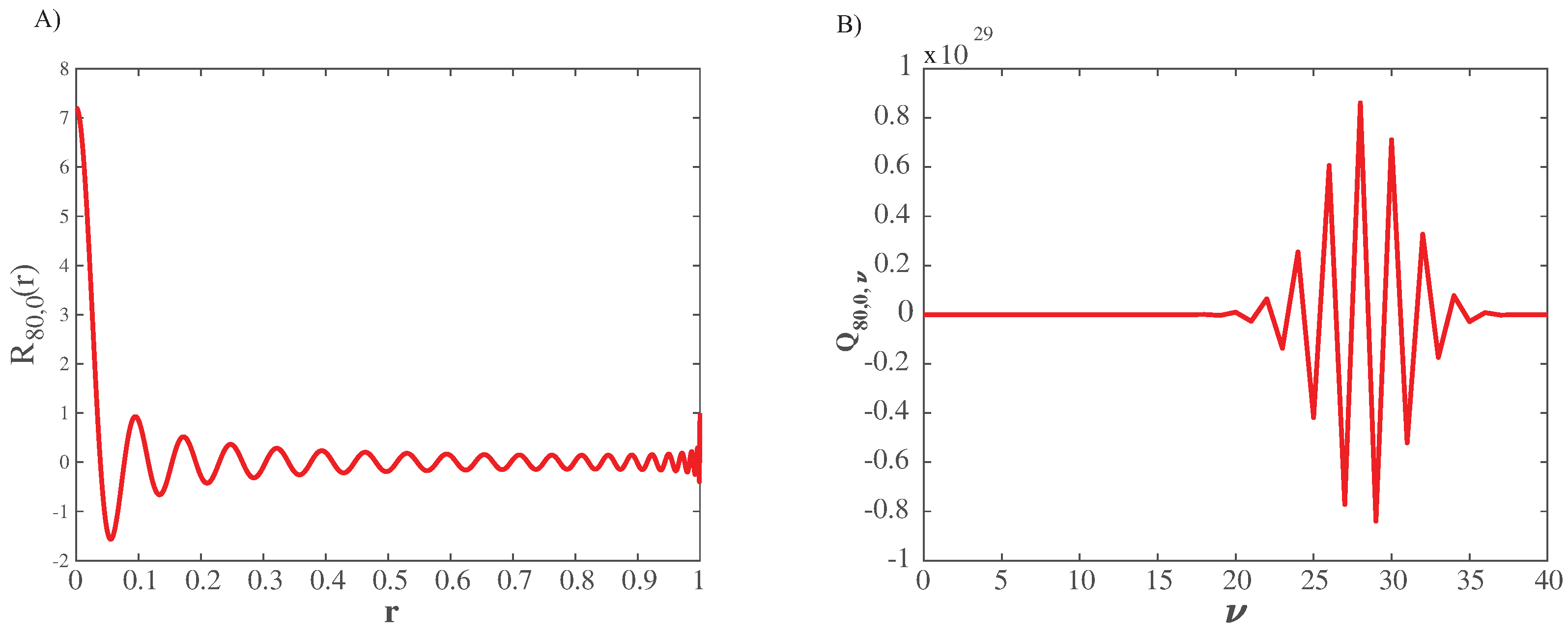
Let us first look at the radial polynomials. $R_{nl}$ is a polynomial of degree n. For large values of n, special care is needed for computing them, and direct application of Equation (9) is bound to numerical instabilities, as described in Figure 1.

The values of $R_{80,0}\left(r\right)$ as a function of r, based on a stable evaluation of the polynomial function vary in the interval $[-1.57,7.20]$, where the largest value is reached for $r=0$. Numerical application of Equation (9) wrongly indicates that $R_{80,l}\left(r\right)$ varies in the interval $[-4149,4\times {10}^{13}]$ (results not shown). This is due to the fact that the coefficients $Q_{80,0,\nu }$ are large (up to ${10}^{29}$), as illustrated in panel B of Figure 1. Those coefficients alternate from positive to negative due to the presence of the term ${(-1)}^{\nu }$, leading to large cancellations and ultimately to a small value for the polynomial. Computing correctly those cancellations requires very high precision usually not available with standard double precision in programming languages. It is possible to use arbitrary precision libraries to solve this issue, but it is in fact not necessary. As was noticed multiple times for the 3D Zernike radial polynomials (see for example [56,57]) the radial polynomial $R_{nl}$ can be expressed as a Jacobi polynomial:

$$R_{nl}\left(r\right)=r^l{P}_{\frac{n-l}{2}}^{(0,l+3/2)}(2r^2-1).$$

(19)

Equation (19) allows the results available in the literature for the Jacobi polynomials to be translated for the 3D radial functions. In particular, we have the following recurrence relation (it was also derived in [54])

$$R_{nl}\left(r\right)=(K_1(n,l)r^2+K_2(n,l))R_{n-2,l}\left(r\right)+K_3(n,l)R_{n-4,l}\left(r\right),$$

(20)

where the coefficients $K_i$ are defined as:

$$\begin{array}{ccc}\hfill k_0& =& (n-l)(n+l+1)(2n-3),\hfill \\ \hfill k_1& =& (2n-1)(2n+1)(2n-3),\hfill \\ \hfill k_2& =& \frac{1}{2}(-2n+1){(2l+1)}^2-\frac{k_1}{2},\hfill \\ \hfill k_3& =& -(n-l-2)(n+l-1)(2n+1),\hfill \\ \hfill K_1(n,l)& =& \frac{k_1}{k_0},K_2(n,l)=\frac{k_2}{k_0},K_3(n,l)=\frac{k_3}{k_0}.\hfill \end{array}$$

(21)

This recursive formula is only valid for $l\le n-4$. This can be addressed by noticing that

$$\begin{array}{ccc}\hfill R_{nn}\left(r\right)& =& r^n,\hfill \\ \hfill R_{n,n-2}\left(r\right)& =& (n+\frac{1}{2})r^n-(n-\frac{1}{2})r^{n-2}.\hfill \end{array}$$

(22)

This recurrence allows for a stable computation of all $R_{nl}\left(r\right)$, even for large orders.

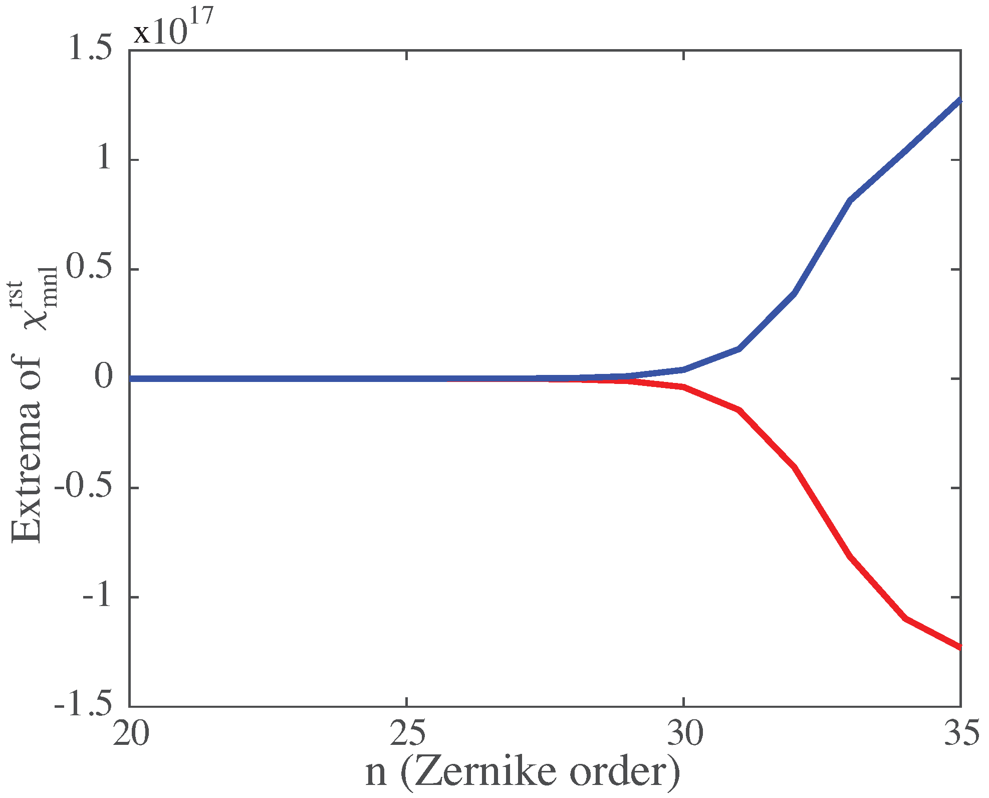
The geometric moments of a shape can be computed accurately even for large orders, see for example [52,53]. Those moments can then be used to evaluate the 3D Zernike moments, as described in the section above. Converting the geometric moments to Zernike moments require, however, that the factor ${\chi }_{nlm}^{rst}$ be computed (where $nlm$ refers to the indices for the Zernike moments, while $rst$ refers to the indices for the geometric moments). As defined in (18), the factors ${\chi }_{nlm}^{rst}$ depend on the coefficients $Q_{nl\nu }$ and therefore they are bound to suffer from the same numerical instabilities. We illustrate this in Figure 2.

As expected, the ${\chi }_{nlm}^{rst}$ vary significantly over a large range of values. This was already observed by Berjón and colleagues in their attempts to parallelize the computation of Zernike moments [46] and is the main reason that the computation of Zernike moments is usually limited to order below $N=50$. One solution to solve this problem would be to derive recurrence relationships for the ${\chi }_{nlm}^{rst}$. Pozo et al. provided such a recurrence. However, their relationships still involve the computations of the factors $Q_{nl\nu }$ (see their Equation (13e)) and as such do not solve the numerical instabilities.

Deng and Gwo [54] proposed a different approach in their attempt to compute Zernike moments for a shape described on a grid, which is to bypass the computation of the geometric moments. In the following, we propose a similar approach for computing Zernike moments for a shape described by a surface-based triangular mesh.

3. Algorithms for Computing the 3D Zernike Moments for a Surface Triangular Mesh

3.1. Zernike Moments over a Shape Defined by a Triangular Surface Mesh

Let us consider a shape S, covering a volume V. The shape is assumed to be represented by a triangle mesh that defines its boundary. Each facet (triangle) T is defined by three vertices A, B and C that are oriented consistently counter-clockwise when seen from the exterior of the shape. As the Zernike polynomials are complete and orthonormal over the unit ball $\mathbb{B}$, the shape is assumed to fit within this ball. This is obtained by centering the mesh to the origin O, and scaling the mesh such that the longest distance between a vertex of the mesh and O is set to one.

Assuming that this shape is homogeneous (i.e., represented by a constant scalar field, with the constant set to one), its Zernike moments $c_{nl}^m$ are given by:

$$c_{nl}^m={\int }_V\overline{Z_{nl}^m\left(\mathit{x}\right)}\mathrm{d}\mathit{x},$$

(23)

where n is the order of the moment, l is a non negative integer smaller or equal to n, with the same parity as n, and m an integer with $-l\le m\le l$.

Using the origin O of the coordinate frame as a reference point, each facet T defines a tetrahedron, ${\sigma }_T=(O,A,B,C)$. We set $\mathit{A}=\overrightarrow{OA}$, with similar notations for B and C. As these tetrahedra are oriented, the integral over the whole shape is simply the sum of the integrals over them. Therefore

$$c_{nl}^m=\sum _{{\sigma }_T}\mathrm{sign}\left(V\left({\sigma }_T\right)\right){\int }_{{\sigma }_T}\overline{Z_{nl}^m\left(\mathit{x}\right)}\mathrm{d}\mathit{x}.$$

(24)

The volume of the oriented tetrahedron is given by

$$V\left({\sigma }_T\right)=\frac{1}{6}\det \left(\mathit{A},\mathit{B},\mathit{C}\right)=\frac{1}{6}\left|\begin{array}{ccc}{x}_A& x_B& x_C\\ y_A& y_B& y_C\\ z_A& z_B& z_C\end{array}\right|.$$

3.2. Basic Idea

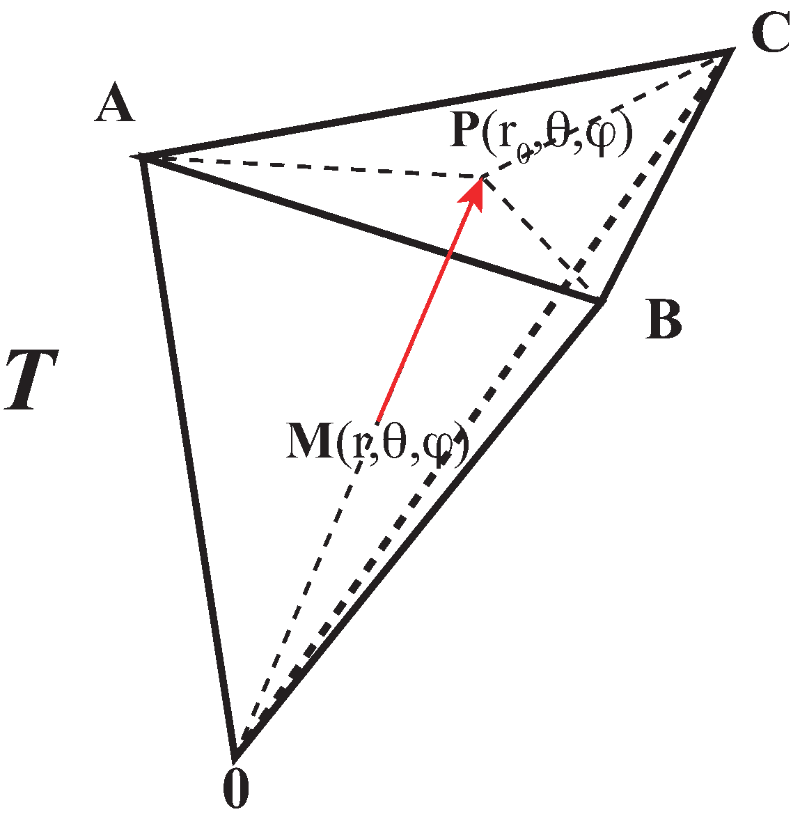
Our task is then to evaluate the integrals of the Zernike polynomials over a tetrahedron ${\sigma }_T=(0,A,B,C)$. The first step is to perform a change of basis, parameterizing any point inside the tetrahedron with respect to its position with respect to the triangle $(A,B,C)$ (see Figure 3).

A point $\mathit{M}$ with spherical coordinates $(r,\theta ,\varphi )$ inside the tetrahedron can be characterized by its projection from the origin to the triangle T. Let $\mathit{P}$ be this point. The spherical coordinates of this point are $(r_0,\theta ,\varphi )$. Note that $r_0$ is a function of $\theta$ and $\varphi$. The integration over the tetrahedron proceeds in two steps, first a radial integration over r from 0 to $r_0$, and then an integration over the triangle only.

$$\begin{array}{cc}\hfill c_{nl}^m\left(T\right)& =\mathrm{sign}\left(V\left({\sigma }_T\right)\right){\int }_{{\sigma }_T}\overline{Z_{nl}^m\left(\mathit{x}\right)}\mathrm{d}\mathit{x}\hfill \\ \hfill & =\frac{3V\left({\sigma }_T\right)}{S\left(T\right)}{\int }_T\frac{1}{r_0^3}\left({\int }_0^{r_0}{r}^2{R}_{nl}\left(r\right)dr\right)\overline{Y_l^m(\theta ,\varphi })\mathrm{d}\mathit{P}.\hfill \end{array}$$

This expression defines a basic 2-step process for evaluating those integrals and therefore the Zernike moments:

(i)

For a given $\mathit{P}$ inside the triangle T with distance $r_0$ to the origin O, compute the radial integral

$$Q_{nl}\left(r_0\right)={\int }_0^{r_0}{r}^2{R}_{nl}\left(r\right)dr.$$

(ii)

Integrate over all points $\mathit{P}$ in the triangle T to get:

$$c_{nl}^m\left(T\right)=\frac{3V\left({\sigma }_T\right)}{S\left(T\right)}{\int }_T\frac{Q_{nl}\left(r_0\right)}{r_0^3}\overline{Y_l^m(\theta ,\varphi })\mathrm{d}\mathit{P}.$$

In the following, we provide recurrence relationships to evaluate the $Q_{nl}$ and describe a numerical way to evaluate exactly the integral in $c_{nl}^m\left(T\right)$, using quadrature.

3.3. Computing the Integrals $Q_{nl}$

We consider the different integrals $S_{nl}^k\left(r\right)$ of the radial functions $R_{nl}\left(r\right)$:

$$S_{nl}^k\left(r_0\right)={\int }_0^{r_0}{r}^k{R}_{nl}\left(r\right)\mathrm{d}r$$

Prata and Rusch have derived relationships for similar integrals for the 2D Zernike radial polynomials [58]. We expand their results here. In Appendix A, we show the following proposition that allows us to compute $S_{nl}^0\left(r_0\right)$:

Proposition 1.

For non negative integers n and l with $l\le n-2$ and $n-l\equiv 0$ (mod 2), the following relationship hold:

$$S_{nl}^0\left(r_0\right)=\frac{2l+3}{(2n+3)(l+1)}\left(R_{n+1,l+1}\left(r_0\right)-R_{n-1,l+1}\left(r_0\right)\right)-\frac{l+2}{l+1}{S}_{n,l+2}^0\left(r_0\right),$$

(25)

and for $l=n$:

$$S_{nn}^0\left(r_0\right)=\frac{r_0^{n+1}}{n+1}.$$

In Appendix B, we then establish a recurrence on the $S_{nl}^k\left(r_0\right)$, in steps of 2 in k:

Proposition 2.

For non negative integers n and l with $l\le n-2$ and $n-l\equiv 0$ (mod 2), and for non negative integer k, the following relationship hold:

$$K_1(n+2,l)S_{nl}^{k+2}\left(r_0\right)=-S_{n+2,l}^k\left(r_0\right)+K_2(n+2,l)S_{nl}^k\left(r_0\right)+K_3(n+2,l)S_{n-2,l}^k\left(r_0\right),$$

(26)

where $K_1$, $K_2$, and $K_3$ are defined in Equation (21).

The special case $k=0$ leads to the following recurrence for the integral $Q_{nl}\left(r_0\right)=S_{nl}^2\left(r_0\right)$:

$$\begin{array}{c}{Q}_{nl}\left(r_0\right)=\frac{(n+2-l)(n+l+3)}{(2n+3)(2n+5)}{S}_{n+2,l}^0\left(r_0\right)\hfill \\ \hfill \hspace{1em}\hspace{1em}\hspace{1em}\hspace{1em}\hspace{1em}\hspace{1em}+\frac{1}{2}\left(\frac{{(2l+1)}^2}{(2n+5)(2n+1)}+1\right)S_{nl}^0\left(r_0\right)+\frac{(n-l)(n+l+1)}{(2n+3)(2n+1)}{S}_{n-2,l}^0\left(r_0\right),\end{array}$$

(27)

for $l=n$, we additionally need:

$$Q_{nn}\left(r_0\right)=\frac{r_0^{n+3}}{n+3}.$$

Finally, we show that for all non negative integer n, and all integer l with $0\le l\le n$ and n and l of the same parity, there exists a polynomial function $U_{nl}$ of degree $n-l$ such that

$$Q_{nl}\left(r_0\right)=r_0^{l+3}{U}_{nl}\left(r_0\right).$$

(28)

The proof is simple. First, we notice that $R_{nl}$ is written as:

$$R_{nl}\left(r_0\right)=r^l{V}_{nl}\left(r_0\right),$$

(29)

where V is a Jacobi polynomial (see Equation (19)) of degree $n-l$. Then

$$Q_{nl}\left(r_0\right)={\int }_0^{r_0}{r}^{l+2}{V}_{nl}\left(r\right)\mathrm{d}r.$$

(30)

Using the polynomial expansion of $V_{nl}$, it is easy to show that $Q_{nl}\left(r_0\right)$ is a polynomial function of degree $n+3$, with $r_0^{l+3}$ as a factor.

3.4. Computing the Integrals $c_{nl}^m\left(T\right)$

Recall that the triangle is defined as $T=(A,B,C)$ and that we need to compute over this triangle the integral

$$c_{nl}^m\left(T\right)=\frac{3V\left({\sigma }_T\right)}{S\left(T\right)}{\int }_T\frac{1}{r_0^3}{Q}_{nl}\left(r_0\right)\overline{Y_l^m(\theta ,\varphi })\mathrm{d}\mathit{P}.$$

Let us define

$$g_{nl}^m\left(\mathit{P}\right)=\frac{1}{r_0^3}{Q}_{nl}\left(r_0\right)\overline{Y_l^m(\theta ,\varphi )}.$$

(31)

Note that there is a function g for all triplets $(n,l,m)$. We need to compute as exactly as possible,

$$\frac{1}{S\left(T\right)}{\int }_T{g}_{nl}^m\left(\mathit{P}\right)\mathrm{d}\mathit{P}.$$

This integral can be approximated with a 2D quadrature [59]

$$\frac{1}{S\left(T\right)}{\int }_T{g}_{nl}^m\left(\mathit{P}\right)\mathrm{d}\mathit{P}\approx \sum _{i=1}^L{w}_i{g}_{nl}^m({\alpha }_{i}A+{\beta }_{i}B+{\gamma }_{i}C),$$

(32)

The sum is computed over $N_p$ points on the triangle, with each point $P_i$ defined by its barycentric coordinates $({\alpha }_i,{\beta }_i,{\gamma }_i)$ with respect to $(A,B,C)$, and $w_i$ is a weight. The points and weights are said to define a quadrature rule. A rule is said to be of strength N if it is capable of exactly integrating any polynomial of maximal degree N over the domain (here the triangle). To apply such a scheme for our application, we need to consider two elements:

(a)

Exactness. As mentioned above, a 2D quadrature may be exact if it is applied on a polynomial. This is our case. Indeed, recall that $Q_{nl}\left(r_0\right)$ is a polynomial function of degree $n+3$, with $r_0^{l+3}$ as a factor. The function g can then be rewritten as

$$\begin{array}{cc}\hfill g_{nl}^m\left(\mathit{x}\right)& =\frac{1}{r^3}{Q}_{nl}\left(r\right)\overline{Y_l^m(\theta ,\varphi })\hfill \\ \hfill & =r^l{U}_{nl}\overline{Y_l^m(\theta ,\varphi })\hfill \\ \hfill & =U_{nl}\overline{e_l^m\left(\mathit{x}\right)},\hfill \end{array}$$

where $e_l^m\left(\mathit{x}\right)$ are the harmonic polynomials (see Equation (5)). As $U_{nl}$ is of degree $n-l$ and $e_l^m$ is of degree l, the function g is a 2D polynomial function of degree n. A quadrature rule of strength n will therefore integrate g exactly.

(b)

Number of points for the quadrature, while it is well known that an n-point Gaussian rule is exact for all polynomials of degree up to $2n-1$ in one dimension, the situation is more complex in higher dimensions. Xiao and Gimbutas [60] proposed an empirical rule for the minimal number of points $N_p^{min}$ to integrate exactly a polynomial of order n:

$$N_p^{min}=⌈\frac{(n+1)(n+2)}{6}⌉.$$

3.5. Two Algorithms for Computing Zernike Moments

The previous subsections provide the elements for computing the contribution of one triangle of a surface mesh to the 3D Zernike moments of the shape enclosed with this mesh. We summarize those elements in Algorithm 1.

Algorithm 1Zernike moments associated with one triangle of a surface mesh

procedureTRIANGLE($N,A,B,C,R$)     Input: N: The maximum order for the 3D Zernike moments. $A,B,C$: The three vertices defining the triangle. R: The 2D quadrature rule     Initialize: $N\left(R\right)$ number of points in R. Initialize $c_{nl}^m\left(T\right)=0$. Compute V, the signed volume of the tetrahedron $(O,A,B,C)$     for $i=1,\dots ,N\left(R\right)$ do         (1) Define $(r_i,{\theta }_i,{\varphi }_i)$ for point ${\mathit{P}}_i$ in the quadrature rule.         (2) Evaluate $Q_{nl}\left(r_i\right)$ over all $n\in [0,N]$, l with $0\le l\le n$ and n and l of same parity         (3) Evaluate $\overline{Y_l^m({\theta }_i,{\varphi }_i)}$ for all l with $0\le l\le N$ and all m with $0\le m\le l$         (4) Compute all $g_{nl}^m\left({\mathit{P}}_i\right)$ based on Equation (31)         (5) Update $c_{nl}^m\left(T\right)=c_{nl}^m\left(T\right)+3V{w}_i{g}_{nl}^m\left({\mathit{P}}_i\right)$     end for     Output: The Zernike moments $c_{nl}^m\left(T\right)$ associated with triangle $(A,B,C)$. end procedure

Briefly, given a quadrature rule R defined by a set of weighted points ${\mathit{P}}_i$, the algorithm proceeds by computing the functions $g_{nl}^m\left({\mathit{P}}_i\right)$ over all those weighted points, and then accumulating the results based on the quadrature rule given by Equation (32). The functions $g_{nl}^m\left({\mathit{P}}_i\right)$ are computed from the $Q_{nl}^m\left(r_i\right)$ at $r_i$, the radial distance of ${\mathit{P}}_i$, and from the $Y_l^m({\theta }_i,{\varphi }_i)$, at the inclination angle ${\theta }_i$ and azimuthal angle ${\varphi }_i$ of ${\mathit{P}}_i$. The corresponding procedure is defined as TRIANGLE. Details on its implementation are provided in the section below.

Given the procedure TRIANGLE, there are two possible algorithms that can then be used to compute the Zernike moments of a shape defined by a surface triangle mesh, one for an exact computation, and one for finite precision. We summarize them in Algorithm 2 and Algorithm 3, respectively.

Algorithm 2Exact Zernike moments for surface triangular meshes

Input: The triangular mesh with M facets supposed to fit inside the unit ball. The maximum order N for the 3D Zernike moments. Initialize: Given N, choose the 2D quadrature rule R to be applied on all triangles. Initialize $c_{nl}^m=0$ for$k=1,\dots ,M$do     (1) Define $(A,B,C)$ the three vertices of triangle k.     (2) Compute $c_{nl}^m\left(T\right)=$ TRIANGLE($N,A,B,C,R$)     (3) Update $c_{nl}^m=c_{nl}^m+c_{nl}^m\left(T\right)$. end for Output: The exact Zernike moments $c_{ln}^m$ of the shape.

3.5.1. Exact Zernike Moments for Shapes Described by Surface Triangular Meshes

As described on the previous subsection, the 2D quadrature rule of strength N will define exact Zernike moments of order up to N on any triangle of the surface mesh. For a given N, if a quadrature rule R with this strength exists, it is then sufficient to use the procedure TRIANGLE defined in Algorithm 1 on all triangles of the surface mesh and then accumulate the results. As described below, we were able to generate quadrature rules for N up to 101. The corresponding algorithm has a complexity of order $O(M\times N^5)$, where M is the number of triangles in the mesh and N the Zernike order. This can be derived as follows. The computation is performed independently on all triangles of the mesh, hence the factor M. For each facet, we need a quadrature rule R of strength N, which itself requires a number of points $N_R$ that is empirically of order $N^2$ (see for example [60]). As $N^3$ functions $g_{nl}^m$ need to be evaluated for each point in the quadrature rule, we get the overall time complexity $O(M\times N^5)$.

Algorithm 3Finite precision Zernike moments for surface triangular meshes

Input: The triangular mesh with M facets supposed to fit inside the unit ball. The maximum order N for the 3D Zernike moments. The tolerance TOL for finite precision computation. Initialize: Set $c_{nl}^m=0$ for$k=1,\dots ,M$do     (1) Define $(A,B,C)$ the three vertices of triangle k.     (2) Compute $c_{nl}^m\left(T\right)=$ TRIANGLEREC($N,A,B,C,TOL$)     (3) Update $c_{nl}^m=c_{nl}^m+c_{nl}^m\left(T\right)$. end for Output: The finite precision Zernike moments $c_{ln}^m$ of the shape.

3.5.2. Finite Precision Zernike Moments for Shapes Described by Surface Triangular Meshes

While Algorithm 2 is deemed exact, it suffers from two major limitations. First, it requires quadrature rules with large strengths. Such rules include large number of sampling points, leading to an overall time complexity $O(M\times N^5)$. Quadrature rules, however, are known to converge fast. As such, it is often not necessary to go to the maximum strength that is required for an exact computation. If we are willing to accept a finite precision, a more efficient procedure can be derived, as described in Algorithm 4. Briefly, the Zernike moments $c_{nl}^m$ over a triangle T are evaluated over quadrature rules of increasing strengths. When the difference between those Zernike moments computed over two successive rules falls below a tolerance, the quadrature is deemed to have converged and the computation stops.

Algorithm 4Adaptive computation of Zernike moments associated with one triangle of a surface mesh

procedureINFO = TRIANGLEADAPT($N,A,B,C,TOL$)     Input: N: The maximum order for the 3D Zernike moments. $A,B,C$: The three vertices defining the triangle. The tolerance TOL for finite precision computation.     Initialize: $c_{nl}^m\left(\mathrm{old}\right)=0$     for $R\in \{R_3,\dots ,R_{101}\}$ do         (1) Compute $c_{nl}^m\left(R\right)=$ TRIANGLE($N,A,B,C,R$)         (2) Compute $\mathrm{err}=\left|\right|c_{nl}^m\left(R\right)-c_{nl}^m\left(\mathrm{old}\right)\left|\right|$         (3) If err < TOL, break         (4) Set $c_{nl}^m\left(\mathrm{old}\right)=c_{nl}^m\left(R\right)$     end for     (5) If err < TOL, set INFO = true, otherwise INFO = false.     Output: INFO, and the current Zernike moments $c_{nl}^m\left(R\right)$ associated with triangle $(A,B,C)$. end procedure

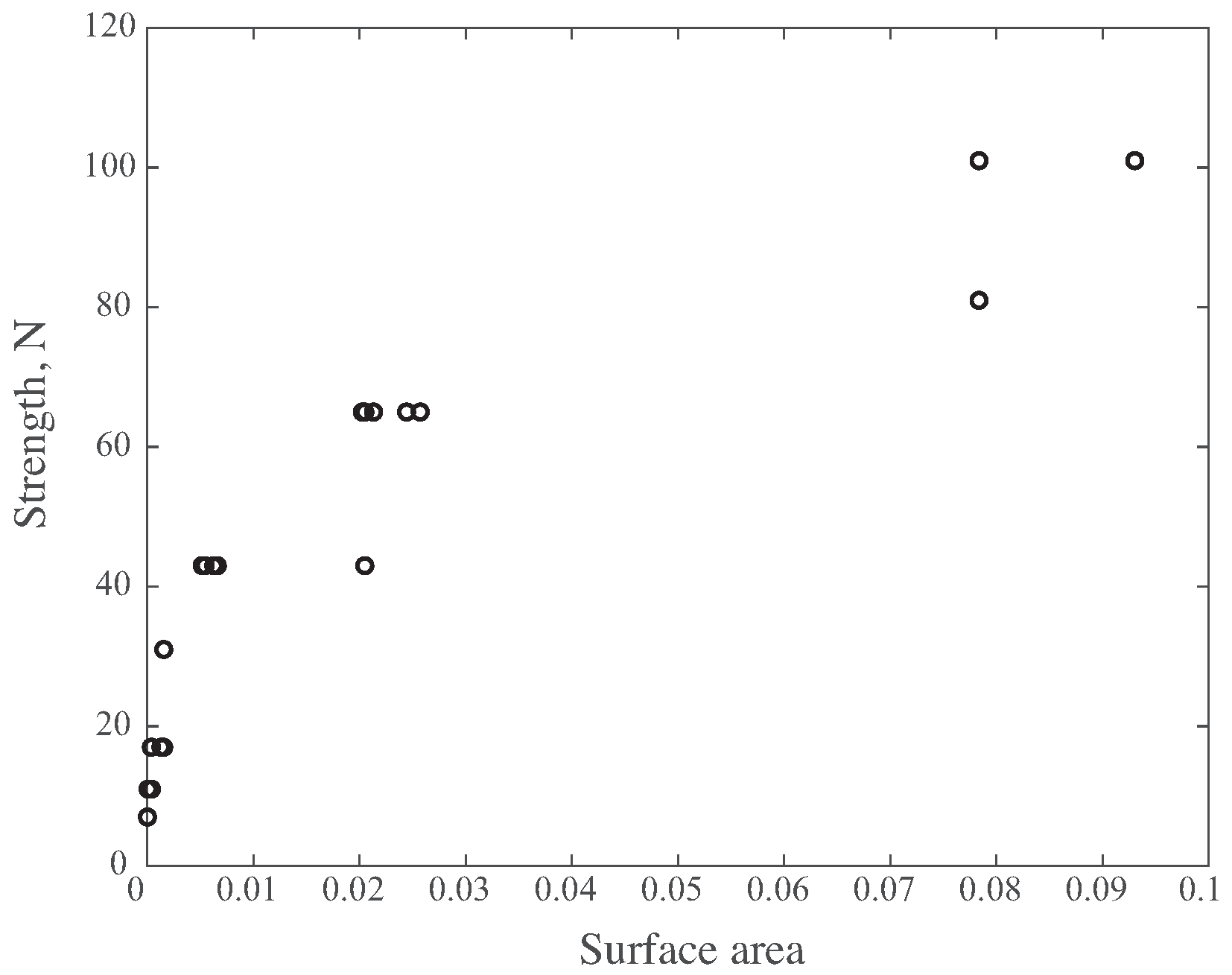
There is a second limitation of Algorithm 1 that remains a problem for Algorithm 4: if the strongest quadrature rule (in our case, 101) is not enough to compute the Zernike moments exactly or to reach the desired tolerance, the algorithms fail. It is expected that the quadrature strength needed to compute correctly the Zernike moments for a tetrahedron $(O,A,B,C)$ is related to the size of the corresponding triangle $(A,B,C)$. To verify this assumption, we performed the following experiment. We considered 8 different discrete spheres represented with a triangular surface mesh. The first mesh corresponds to an icosahedron, while the following meshes are generated consecutively by successive subdivisions of all triangles of the previous mesh. All those meshes are scaled so that they fit within the unit ball, with a maximum radius of 0.75. We applied algorithm TRIANGLEADAPT to all facets of all those meshes, and compared the maximum order on exit of the procedure to the surface area of the corresponding triangle. Results are shown in Figure 4.

Figure 4 shows that the larger the triangle, the higher the strength of the quadrature. This result hints to a simple procedure to alleviate the second problem described above: if the procedure TRIANGLEADAPT fails, split the triangle into four smaller triangles, possibly recursively. We have implemented this procedure in Algorithm 5.

Algorithm 5Recursive computation of Zernike moments associated with one triangle of a surface mesh

procedureTRIANGLEREC($N,A,B,C,TOL$)     Input: N: The maximum order for the 3D Zernike moments. $A,B,C$: The three vertices defining the triangle. The tolerance TOL for finite precision computation.     (1) Compute (INFO, $c_{nl}^m\left(T\right)=$ TRIANGLEADAPT($N,A,B,C,TOL)$     if INFO==true then         (2) RETURN $c_{nl}^m\left(T\right)$     else         (3) Find $A^{\prime },B^{\prime },C^{\prime }$ the middle points of segment $BC$, $AC$, $CA$         (4) Compute            (a) $c_{nl}^m\left(1\right)=$ TRIANGLEREC($N,A,C^{\prime },B^{\prime },TOL$)            (b) $c_{nl}^m\left(2\right)=$ TRIANGLEREC($N,B,A^{\prime },C^{\prime },TOL$)            (c) $c_{nl}^m\left(3\right)=$ TRIANGLEREC($N,C,B^{\prime },A^{\prime },TOL$)            (d) $c_{nl}^m\left(4\right)=$ TRIANGLEREC($N,A^{\prime },B^{\prime },C^{\prime },TOL$)         (5) RETURN $c_{nl}^m\left(T\right)=c_{nl}^m\left(1\right)+c_{nl}^m\left(2\right)+c_{nl}^m\left(3\right)+c_{nl}^m\left(4\right)$.     end if end procedure

The finite precision algorithm for computing the Zernike moments of a shape to a finite precision TOL is then given by Algorithm 3.

4. Reconstructing a Shape from Its 3D Zernike Moments

Recall that once a shape S has been characterized with its Zernike moments $c_{nl}^m$, its density $\rho \left(\mathit{x}\right)$ at any point $\mathit{x}$ in ${\mathbb{R}}^3$ can be reconstructed using Equation (14)

$$\begin{array}{cc}\hfill \rho \left(\mathit{x}\right)& =\sum _n^N\sum _l\sum _{m=-l}^l{c}_{nl}^m{Z}_{nl}^m\left(\mathit{x}\right)\hfill \\ \hfill & =\sum _n^N\sum _l\sum _{m=-l}^l{c}_{nl}^m\sqrt{2n+3}{R}_{nl}\left(r\right)Y_l^m(\theta ,\varphi ),\hfill \end{array}$$

(33)

where $(r,\theta ,\varphi )$ are the spherical coordinates of $\mathit{x}$. The reconstruction is exact when $N\to +\infty$, while the Zernike moments $c_{nl}^m$ and the Zernike polynomials are complex, the reconstruction $\rho \left(\mathit{x}\right)$ is real.

The equation above defines a simple algorithm for reconstructing the shape density in ${\mathbb{R}}^3$. If the points $\mathit{x}$ are chosen to be the nodes of a 3D grid, a surface mesh can then be reconstructed using the marching tetrahedron algorithm [49]. We note, however, that special care is needed when evaluating the radial polynomials $R_{nl}\left(r\right)$ and the spherical harmonics $Y_l^m(\theta ,\varphi )$ to avoid numerical instabilities when n is large. This is described below in the Implementation section.

5. Implementation

The computation of the Zernike moments of a shape described by a surface triangular mesh is performed either with the exact Algorithm 2 or with the finite precision Algorithm 3. Both algorithms rely heavily on the functions that compute the geometric moment associated with a triangle of the mesh, TRIANGLE (Algorithm 1) and TRIANGLEREC (Algorithm 5). We identify three elements that are essential for the implementations of those algorithms:

(1)

Definitions of the quadrature rules for integration on a triangle,

(2)

Efficient computations of $R_{nl}\left(r\right)$ and $Q_{nl}\left(r\right)$,

(3)

Efficient computations of the spherical harmonics $Y_l^m(\theta ,\varphi )$.

We describe the specifics for those three elements.

5.1. Quadrature Rules for Integration over a Triangle

A quadrature rule over a domain D is defined through its ability to integrate exactly over D the set of basis polynomials of degree $n\le N$, ${\mathbb{P}}^N$. This set has an infinite number of representations. The simplest of those representations is to consider monomials. In two dimensions, those monomials are $\{x^i{y}^j,i+j\le N\}$. Unfortunately, monomials of high degrees are extremely sensitive to small perturbations. This gives rise to systems which are poorly conditioned and hence difficult to solve numerically [61]. We have used instead the approach of Witherden and Vincent [62] to derive our quadrature rules. They proposed to use orthogonal polynomials ${\psi }_{ij}$ as a basis of ${\mathbb{P}}^N$ with $i+j\le N$, such that

$${\int }_D{\psi }_{ij}\left(\mathit{x}\right){\psi }_{kl}\left(\mathit{x}\right)\mathrm{d}\mathit{x}={\delta }_{ik}{\delta }_{jl},$$

where $\delta$ is the Kronecker delta. By taking ${\psi }_{00}\left(\mathit{x}\right)=1/c$, they define the error associated with a quadrature rule with $N_p$ points as:

$${\chi }^2\left(N\right)=\sum _{ij}{\left\{\sum _{k=1}^{N_p}{w}_k{\psi }_{ij}\left({\mathit{x}}_k\right)-c{\delta }_{i0}{\delta }_{j0}\right\}}^2.$$

(34)

In Witherden and Vincent’s schemes, constructing an $N_p$ rule of strength N is then akin with finding a set of points ${\mathit{x}}_k$ and associated weights $w_k$ that minimize ${\chi }^2\left(N\right)$. They provided an open source software package, PolyQuad (available on 23 September 2022 at https://github.com/PyFR/Polyquad) for this task. We have run PolyQuad for strengths between 3 and 101 to generate the quadrature rules that we have used for computing Zernike moments. In Appendix C, we list the number of points required for each strength. The actual number of points is found to be similar to the empirical bound of $\lceil (N+1)(N+2)/6\rceil$ proposed by Xiao and colleagues [60].

5.2. Efficient Computations of the Polynomials $R_{nl}\left(r\right)$ and $Q_{nl}\left(r\right)$

As described in Section 2, it is crucial to compute the radial polynomials $R_{nl}\left(r\right)$ accurately. A naive computation using its monomial decomposition does not achieve this accuracy for high order n. Instead, we have used the recurrence (20) that is derived from the properties of Jacobi polynomials (see Section 2).

The polynomial $Q_{nl}\left(r\right)$ are the indefinite integrals of the radial polynomials $R_{nl}\left(r\right)$ weighted by $r^2$. Properties 1 and 2 (major results of this paper) provide simple recurrence for computing those integrals.

5.3. Efficient Computations of the Spherical Harmonics $Y_l^m(\theta ,\varphi )$

The spherical harmonics are related to the associated Legendre polynomials, from which they inherit many properties. In particular, they can be computed recursively. We have used the following recurrences:

Proposition 3.

For non negative integers l and m with $0\le m\le l$ the following relationships hold:

(i) 

For $l>1$ and $0\le m<l-1$:

$$\begin{array}{c}{Y}_l^m(\theta ,\varphi )=\sqrt{\frac{(2l+1)(2l-1)}{(l+m)(l-m)}}cos\theta Y_{l-1}^m(\theta ,\varphi )\hspace{1em}\hspace{1em}\hspace{1em}\hspace{1em}\hspace{1em}\hspace{1em}\hspace{1em}\hspace{1em}\hspace{1em}\hspace{1em}\hspace{1em}\hspace{1em}\hfill \\ \hfill \hspace{1em}\hspace{1em}\hspace{1em}\hspace{1em}\hspace{1em}\hspace{1em}\hspace{1em}\hspace{1em}\hspace{1em}\hspace{1em}\hspace{1em}\hspace{1em}-\sqrt{\frac{(2l+1)(l+m-1)(l-m-1)}{(2l+3)(l+m)(l-m)}}{Y}_{l-2}^m(\theta ,\varphi ).\end{array}$$

(35)

(ii) 

For $l>0$ and $m=l-1$:

$$Y_l^{l-1}(\theta ,\varphi )=\sqrt{2l+1}cos\theta Y_{l-1}^{l-1}(\theta ,\varphi ).$$

(36)

(iii) 

For $l>0$ and $m=l$:

$$Y_l^l(\theta ,\varphi )=-sin\theta \sqrt{\frac{2l+1}{2l}}{\mathrm{e}}^{i\varphi }{Y}_{l-1}^{l-1}(\theta ,\varphi ).$$

(37)

With the initialization $Y_0^0(\theta ,\varphi )=1/\sqrt{4\pi }$, Equations (35)–(37) provide an efficient scheme for computing all spherical harmonics at angles $(\theta ,\varphi )$.

5.4. Efficient Reconstruction of a Shape from Its Zernike Moments

As given by Equation (33), the Zernike moments can be used to reconstruct a field $\rho \left(\mathit{x}\right)$ for $\mathit{x}$ within the unit ball. This field is expected to be 0 or 1 outside or inside of the shape to be reconstructed, respectively. The summation over all orders of the Zernike moment is performed using the same recursions that are used to compute the Zernike moments. A triangulated surface is then constructed as an isosurface of this field, usually at the level $\rho \left(\mathit{x}\right)=0.5$. We chose the regularized marching tetrahedra algorithm [50] to generate this surface.

6. Numerical Results

We have derived new algorithms for computing the Zernike moments of a shape represented by a surface mesh, respectively. In this section, we analyze the computational complexity of both. We propose experiments to measure the numerical stability of the programs that implement these algorithms. Finally we show examples of shape reconstructions based on high order Zernike moments derived with these algorithms.

6.1. Accuracy of the Computed 3D Zernike Moments: Comparison with Other Algorithms

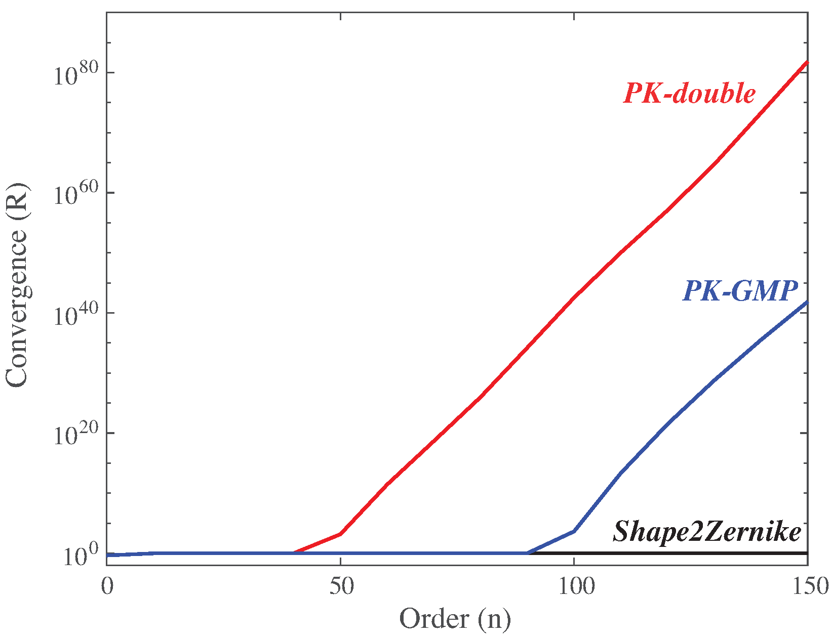
In the specific case of a homogeneous shape, the version of the Parseval’s theorem for Zernike moments allows us to monitor the convergence of the computations of these moments. Indeed, for an 0 shape, $f^2\left(\mathit{x}\right)$ is constant. Taking this constant to 1, we get

$$\sum _{n=0}^{\infty }\sum _l\sum _{m=-l}^l{\left|c_{nl}^m\right|}^2={\int }_{\mathbb{B}}{f}^2\mathrm{d}\mathit{x}={\int }_V\mathrm{d}\mathit{x}.$$

In parallel, we have:

$$c_{00}^0={\int }_{\mathbb{B}}{f}^2\left(\mathit{x}\right)Z_{00}^{0}dx=\sqrt{\frac{3}{4\pi }}{\int }_V\mathrm{d}\mathit{x}.$$

Therefore,

$$\sum _{n=0}^{\infty }\sum _l\sum _{m=-l}^l{\left|c_{nl}^m\right|}^2=\sqrt{\frac{4\pi }{3}}{c}_{00}^0.$$

(38)

This implies that the Euclidean norm of the Zernike moments up to order N converges to a factor times $\sqrt{c_{00}^0}$ when N increases, which can be used as a test for the numerical stability of the algorithm. Figure 5 shows this convergence for three different programs for computing the Zernike moments, for maximum order up to 150. All calculations are performed on a discretized sphere represented with a mesh of 20,480 triangles (this mesh was generated from the regular icosahedron with 5 consecutive subdivisions of its facet). This sphere is scaled inside the unit ball such that its maximum radius is $r_0=0.75$. The computations were performed on one thread of a Linux server, with a Xeon Platinum 8168 CPU running at 2.7 GHz.

The first program we use implements the computation of the Zernike moments from the geometric moments of the shapes, using the PK algorithm proposed by Pozo et al. [52], with the modified computation of geometric moments proposed by Koehl [53]. All calculations are performed in double precision. As seen in Figure 5, the convergence breaks down at $N=50$; this is similar to the behavior described by Pozo et al. [52] for their own algorithm, and for the alternate algorithm proposed by Novotni and Klein [22]. We believe, in par with their comments, that the divergence is due both to the summations needed for computing the Zernike moments from the geometric moments that involve terms with alternating signs, and to the accuracy with which both high order monomials and high order binomial coefficients are computed.

One option to circumvent this divergence problem is to increase the precision with which real numbers are represented. The second program we have used is a rewrite of the first program that makes full use of the GNU Multiple Precision (GMP) library. The calculations of the geometric moments involve linear recursions; they can therefore be performed using arbitrary precision integer arithmetics. The conversion to Zernike moments is then performed with floats with 512 bit accuracy. As seen in Figure 5, this full GMP implementation converges for order up to 100. It still fails, however, for order higher than 100. In addition, the computational cost however is high: the full GMP calculation required 4200 s for $N=100$, while the double precision float calculation only requires 100 s.

The third program with have used is Shape2Zernike implementing Algorithm 3 introduced in this paper. Compared to the two other programs, it computes the Zernike moments directly, without relying on the geometric moments. It is found to be stable over a wide range of order (we have tested it up to order 400). It has a moderate computational cost (220 s).

6.2. Accuracy of the Computed 3D Zernike Moments: Comparison with Exact Values

In the previous section, we have looked at the stability of the algorithm. To assess its accuracy, we considered a sphere centered at the origin with radius $r_0$ with $0<r_0<1$. The Zernike moments of such a sphere are defined as

$$c_{nl}^m=\sqrt{2n+3}{\int }_0^{r_0}\mathrm{d}r{r}^2{R}_{nl}\left(r\right){\int }_0^{\pi }sin\theta \mathrm{d}\theta {\int }_0^{2\pi }\mathrm{d}\varphi \overline{Y_l^m(\theta ,\varphi )}.$$

Let us recall first the orthonormality of the spherical harmonics:

$${\int }_0^{\pi }sin\theta \mathrm{d}\theta {\int }_0^{2\pi }\mathrm{d}\varphi Y_l^m(\theta ,\varphi )\overline{Y_{l^{\prime }}^{m^{\prime }}(\theta ,\varphi )}={\delta }_{m{m}^{\prime }}{\delta }_{l{l}^{\prime }}.$$

(39)

Applying this equation for $m^{\prime }=0$ and $l^{\prime }=0$, and using the fact that $Y_0^0=1/\sqrt{4\pi }$, we get

$${\int }_0^{\pi }sin\theta \mathrm{d}\theta {\int }_0^{2\pi }\mathrm{d}\varphi Y_l^m(\theta ,\varphi )=\sqrt{4\pi }{\delta }_{m0}{\delta }_{l0}.$$

The integral on the left is therefore non zero only for $l=0$ and $m=0$, in which case it is equal to $\sqrt{4\pi }$. The Zernike moments $c_{nl}^m$ of a sphere are then non zero only for $l=0$ and $m=0$:

$$\begin{array}{c}\hfill c_{n0}^0\left(ref\right)=\sqrt{4\pi }\sqrt{2n+3}{\int }_0^{r_0}{r}^2{R}_{n0}\left(r\right)dr=\sqrt{4\pi }\sqrt{2n+3}{Q}_{n0}\left(r_0\right),\end{array}$$

(40)

where $Q_{n0}$ is defined in Equation (27). Note finally that, as $l=0$ is even, n needs also to be even.

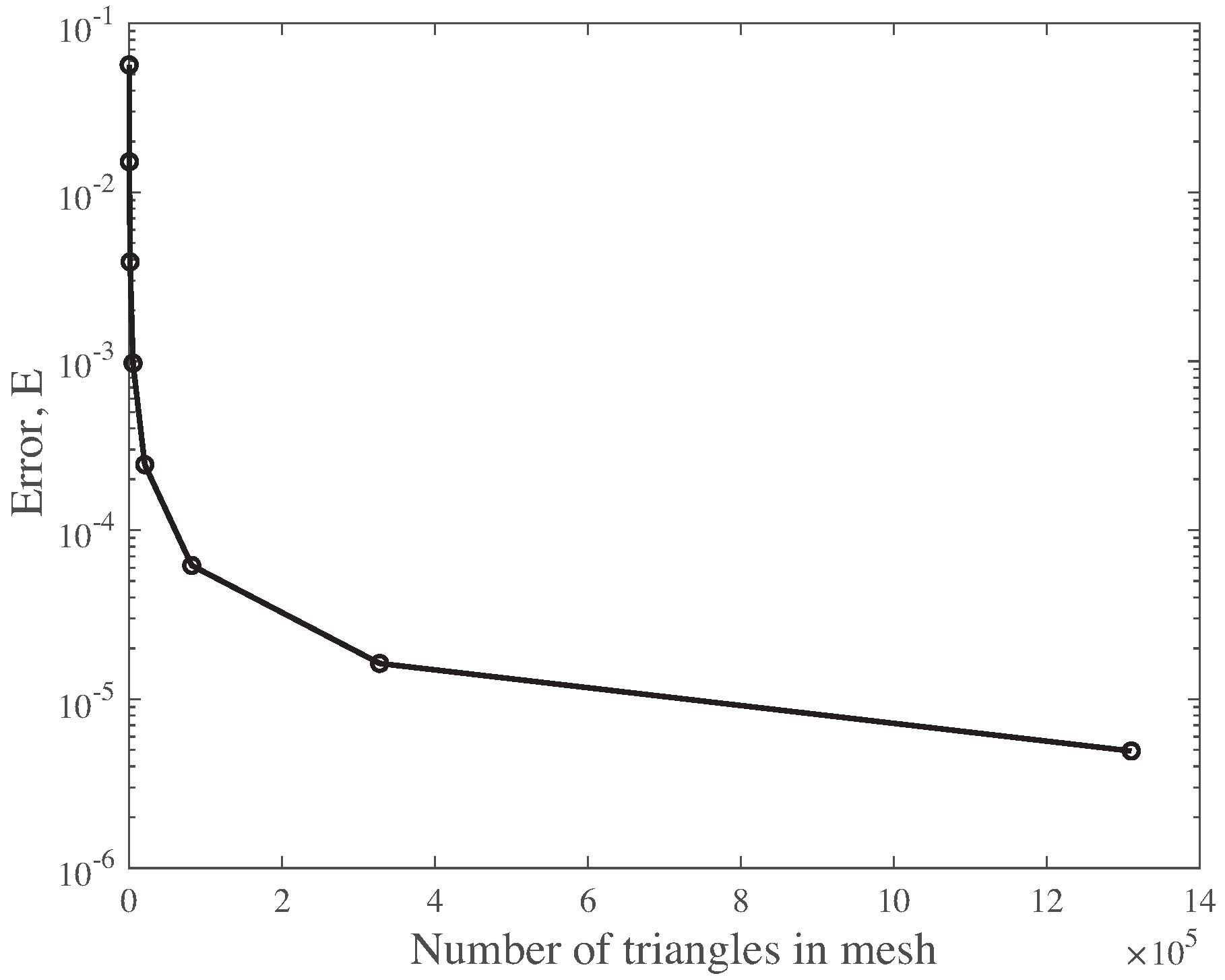
The exact algorithm (Algorithm 2) and the finite precision algorithm (Algorithm 3, with TOL set to ${10}^{-8}$) have been applied to compute the Zernike moments of order 100 of triangle meshes representing the sphere with radius $r_0=0.75$. Those meshes were constructed from successive subdivisions of the icosahedron, leading to eight meshes with 80 facets for the coarser, and 1,310,720 facets for the finer. The error has been measured using the Euclidean distance between the Zernike moments computed numerically with the exact or with the finite precision algorithm, and the reference Zernike moments computed from Equation (40), divided by the Euclidean modulus of the reference:

$$E=\frac{\sqrt{{\sum }_{nlm}{\left|c_{nl}^m-c_{nl}^m\left(ref\right)\right|}^2}}{\sqrt{{\sum }_{nlm}{\left|c_{nl}^m\left(ref\right)\right|}^2}}.$$

Results for the exact algorithms are shown in Figure 6. Those for the finite precision algorithm are 0. As expected, the error decreases as the number of triangles in the mesh decrease. The meshes we have used do not represent the sphere exactly; the representation improves, however, as the number of triangles increase. The errors observed in Figure 6 relate to this discretization error. The error associated with computing the Zernike polynomial are minimal compared to those.

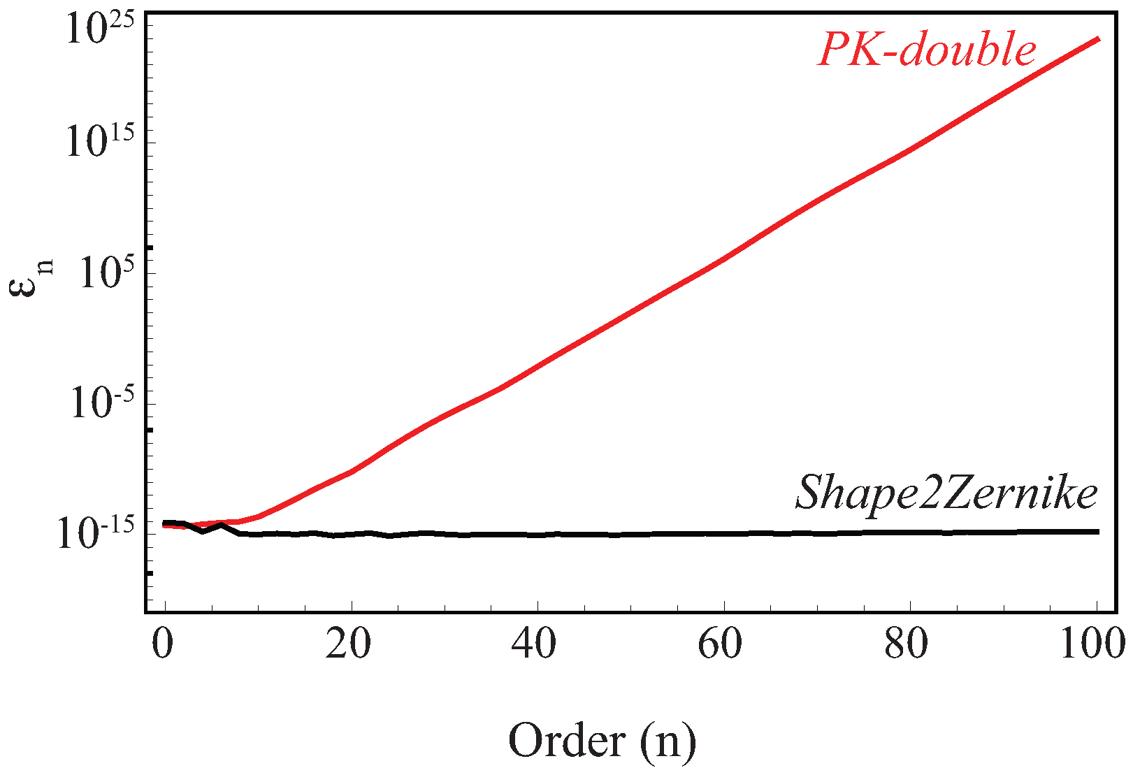
As discussed above, while it is possible to compute the Zernike moments for a sphere analytically, representation of a sphere with a discrete 3D mesh is only approximate. To further analyze the accuracy of our algorithms, we considered a second simple shape, a cube. Such a cube can be represented exactly with a triangular mesh: we considered a cube with 12 facets aligned with the 0 axes and just fitting in the unit ball (thus with edges of size $2/\sqrt{3}$). There are no analytical formula for the Zernike moments of a cube. However, they can be computed symbolically using a symbolic algebra system (we have used Mathematica [63]). To achieve this, we generated the monomial expansion of the Zernike polynomials and then integrated them symbolically over the volume of the cube. This provided an exact symbolic result for each moment which was then evaluated to double precision. We compared the results of the double precision program PK (see above), of the exact algorithm (Algorithm 2), and of the finite precision algorithm (Algorithm 3, with TOL set to ${10}^{-8}$) (both implemented in Shape2Zernike) with those exact values for Zernike moments up to order 100, using the following error function

$${ϵ}_n=\sqrt{{\sum }_l{\sum }_{m=-l}^l{|c_{nl}^m\left(\mathrm{computed}\right)-c_{nl}^m\left(\mathrm{exact}\right)|}^2}.$$

(41)

Results are shown on Figure 7. The two new algorithms perform extremely well at all orders with an error of order ${10}^{-15}$ compared to these exact values.

6.3. Reconstructing a Shape from its 3D Zernike Moments: Example of the Sphere

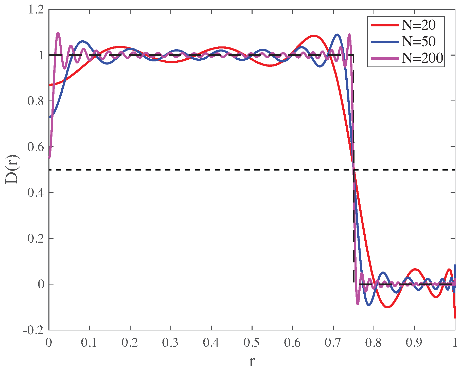
The reconstruction of a shape function $\rho \left(\mathit{x}\right)$ can be carried out starting from Equation (33). For the sphere with radius $r_0$, the triple summation in this equation converges to a step function equal to 1 for $r<r_0$ and 0 for $r>r_0$. We assessed the quality of this reconstruction for the discrete sphere of radius $r_0=0.75$ represented with a triangular mesh with 1,310,720 facets. We computed $D\left(r\right)$ at a set of points $\mathit{x}$ whose spherical coordinates are $(r,0,0)$. In Figure 8, we show $D_r$ for $N=20$, 50 and 200. Note that all reconstructions have a value near 0.5 for $r=r_0$. This observation indicates that general shape reconstruction consists of computing a field over the unit sphere with the field value at a point $\mathit{x}$ being the summation in Equation (33) for $n=0$ up to a maximum preset value N, and then taking the isosurface at level 0.5 of this field to define the surface of the reconstructed object.

6.4. Reconstructing a Shape from Its 3D Zernike Moments: Importance of the Order N

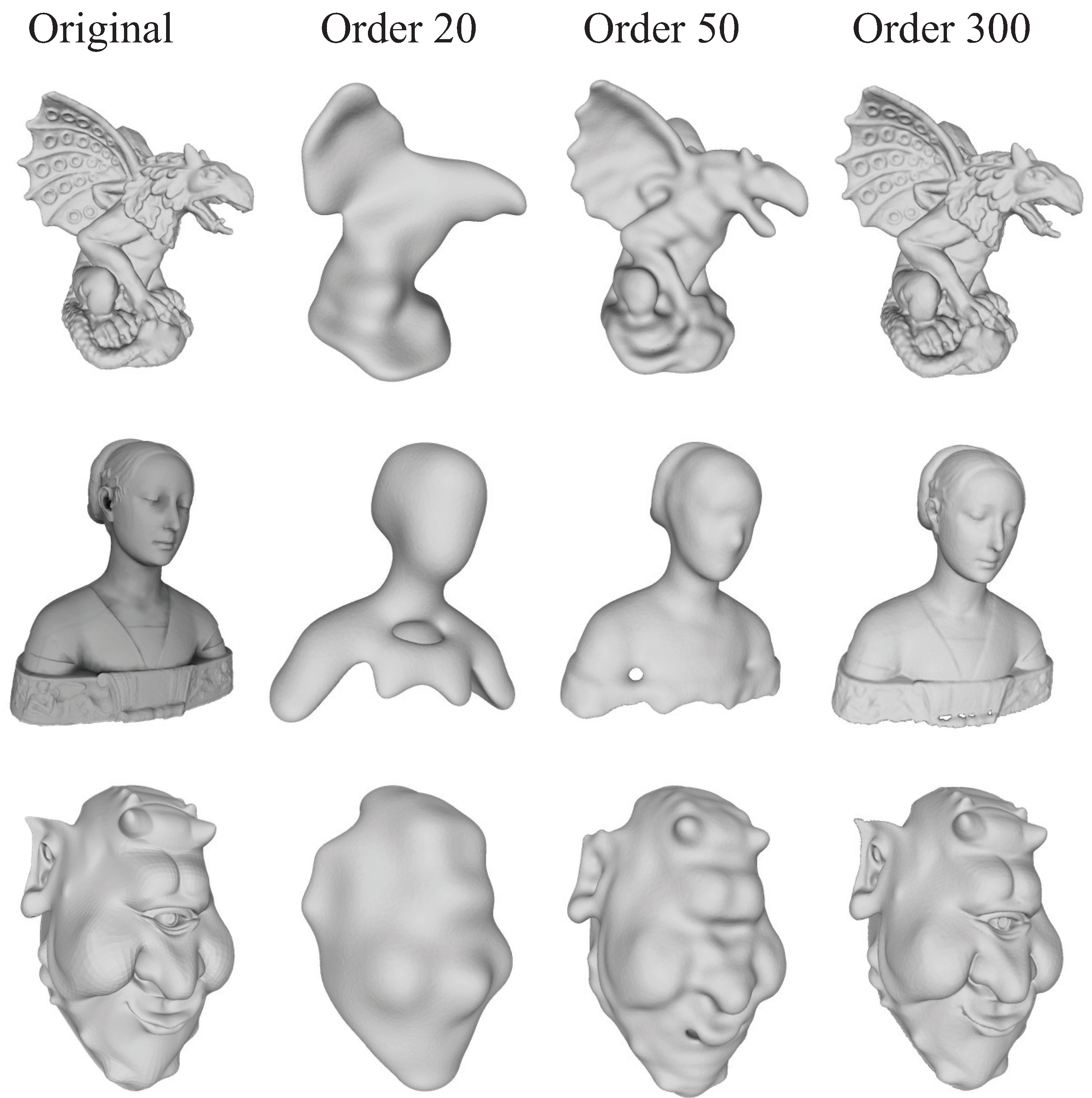
We consider three different experiments for the reconstruction of a shape from its Zernike moments based on generic shapes, Figure 9, on shapes of protein structures, Figure 10, and on shapes of a human organ, the brain, Figure 11.

Figure 9 shows the quality of reconstruction of a shape from its Zernike moments at different orders for standard 3D models from the computer graphics community. The first row corresponds to a model of a gargoyle, available at the repository AIMS@SHAPE (accessed on 23 September 2022) (http://visionair.ge.imati.cnr.it/). The original mesh includes 50,002 vertices and 100,000 triangles. We computed the Zernike moments of this shape using the finite precision algorithm with a tolerance of ${10}^{-8}$, up to order 300. We then reconstructed the shape by computing a field over the unit ball, where each node in the field is assigned a value corresponding to Equation (33), with different orders of N and then identifying the surface of the reconstructed shape with the 0.5 isosurface of this field. The isosurface is built using the regularized marching tetrahedra algorithm [50]. As expected, the quality of the reconstruction depends on the maximum order N considered. For $N=20$, the reconstructed surface only shows the global envelope with no details. For $N=50$, the shape of the gargoyle is better defined; however, fine details are still missing. For example, we do not see any texture in the wings. $N=300$ gives us a more accurate representation of the shape, with fine details within the wings and in the mane of the gargoyle.

The second row corresponds to a statue of the bust of Ippolita Sforza, sculpted by Francesco Laurana. It is available as part of the package MeshLab [64]. The mesh includes 27,861 vertices and 49,954 triangles. We computed its Zernike moments using the finite precision algorithm with a tolerance of ${10}^{-8}$, up to order 300. We then reconstructed its shape using the same procedure described above for the gargoyle, with orders $20,50$, and 300. For $N=20$, the reconstructed bust is incomplete, with no details on its surface. For $N=50$, we start seeing faint features within the face, but the bottom of the bust is still incomplete. $N=300$ gives us a much more accurate representation of the model, especially in the face.

The third row corresponds to the smiling version of Jerry the Ogre, introduced by Carr et al. It is available at the 3D model repository of Keenan Crane (accessed on 23 September 2022) (https://www.cs.cmu.edu/~kmcrane/Projects/ModelRepository/). The mesh includes 27,861 vertices and 49,954 triangles. We computed its Zernike moments using the finite precision algorithm with a tolerance of ${10}^{-8}$, up to order 300. We then reconstructed its shape using the same procedure described above for the gargoyle and the bust by Laurana, with orders $20,50$, and 300. For $N=20$, the reconstructed face of Jerry has no features. For $N=50$, we start seeing faint features within the face; some elements such as the eye are still missing. For $N=300$ the face is reconstructed reasonable 0.

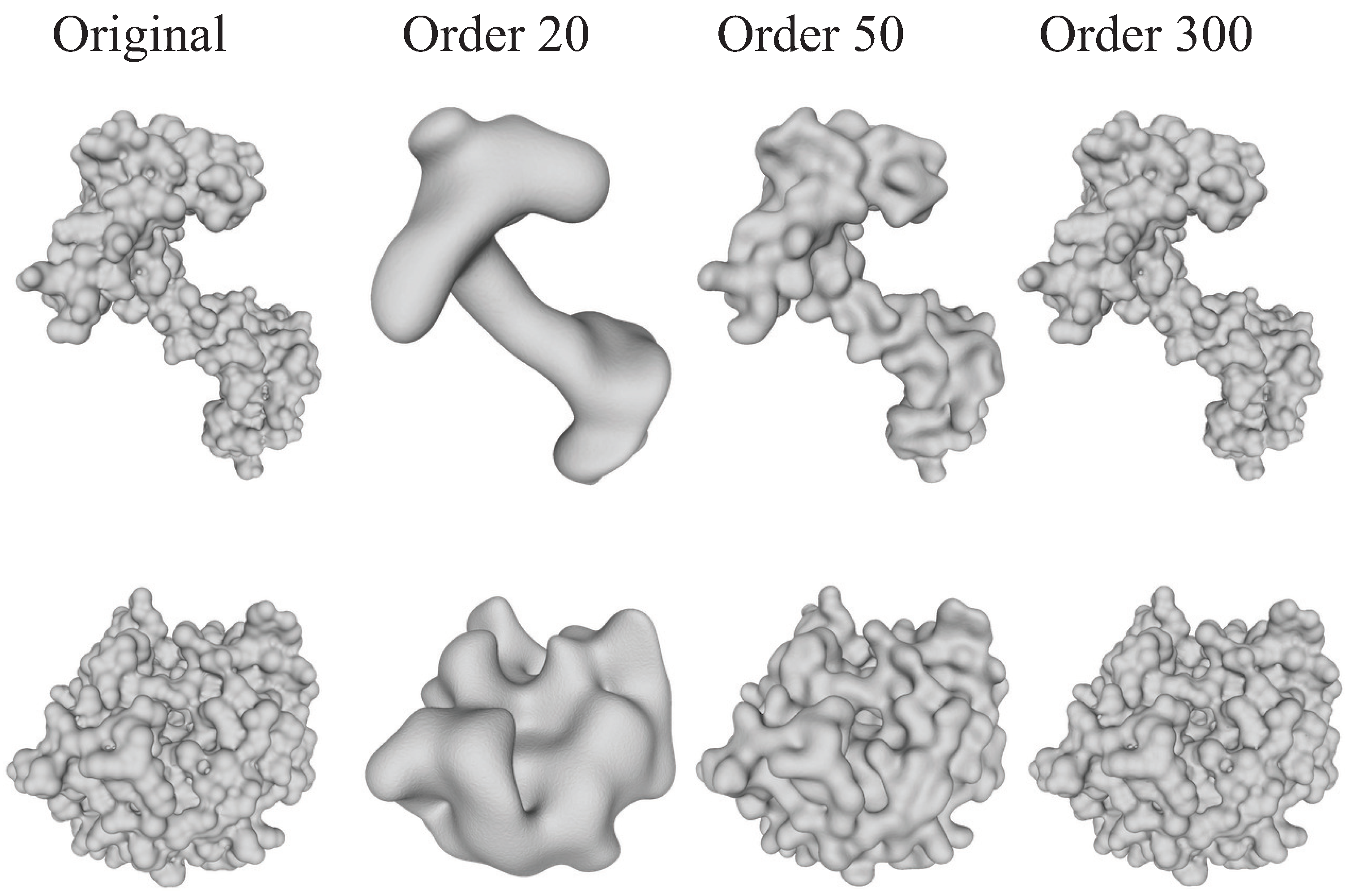
Figure 10 shows the quality of reconstruction of a protein shape from its Zernike moments at different orders. We consider two well studied proteins often used as models in computational structural biology, calmodulin (top row) and a triose phosphate isomerase (bottom row).

Calmodulin is a calcium binding protein expressed in all eukaryotic cells. It is a small protein that consists of two small domains separated by a linker region. The flexibility of this linker is key to the ability of calmodulin to bind to a wide range of substrates [67]. We considered the apo form (without ligand) of the human version of protein available in the Protein Data Bank [32] with the code 1CLL. This conformation is defined as the position of its 1133 atoms. We use the standard model in chemistry of representing a structure as a union of balls, with each ball corresponding to an atom. The surface of this union of ball is represented as its skin surface [68]. It is computed from the boundary of the union of these balls, where the center of a ball is given by the coordinates of the atom, and its radius is set to its van der Waals radius plus a probe radius of $R=1.4$ Å. We generated a quality mesh for the skin surface of calmodulin using the program smesh, described in details in [65,66]. The corresponding triangular mesh includes 203,400 vertices and 406,864 triangles. We computed its Zernike moments using the finite precision algorithm with a tolerance of ${10}^{-8}$, up to order 300. We then reconstructed a shape for calmodulin using the same procedure described above, with orders 20, 50, and 300. Those two domains of calmodulin are clearly separated in the absence of a ligand, as illustrated from its original surface. For $N=20$, the reconstruction shows the position of these two domains. However, it does not include any local features, while some of those features (i.e., the presence of spherical patches) appear for $N=50$, they are only clearly visible at much higher orders, as illustrated here for $N=300$.

Triose phosphate isomerase (TIM) is an enzyme that catalyzes the reversible interconversion of triose phosphate isomers [69]. We considered the chicken version of the TIM protein available in the Protein Data Bank [32] with the code 1TIM. This conformation is defined from the positions of its 1870 atoms. We generated a quality mesh for its skin surface using the same procedure described above for calmodulin. The corresponding triangular mesh includes 398,658 vertices and 797,644 triangles. We then computed its Zernike moments using the finite precision algorithm with a tolerance of ${10}^{-8}$, up to order 300. We reconstructed a shape for TIM using the same procedure described above, with orders 20, 50, and 300. Compared to the example of calmodulin shown above, TIM is a more globular protein. The reconstruction of its shape for $N=20$ shows similar characteristics than the corresponding reconstruction for calmodulin: the overall shape is conserved, without information on local details. In contrast, Reconstructions at $N=50$ and more significantly at $N=300$ show the local features of the surface of TIM, namely the local spherical patches corresponding to its atoms.

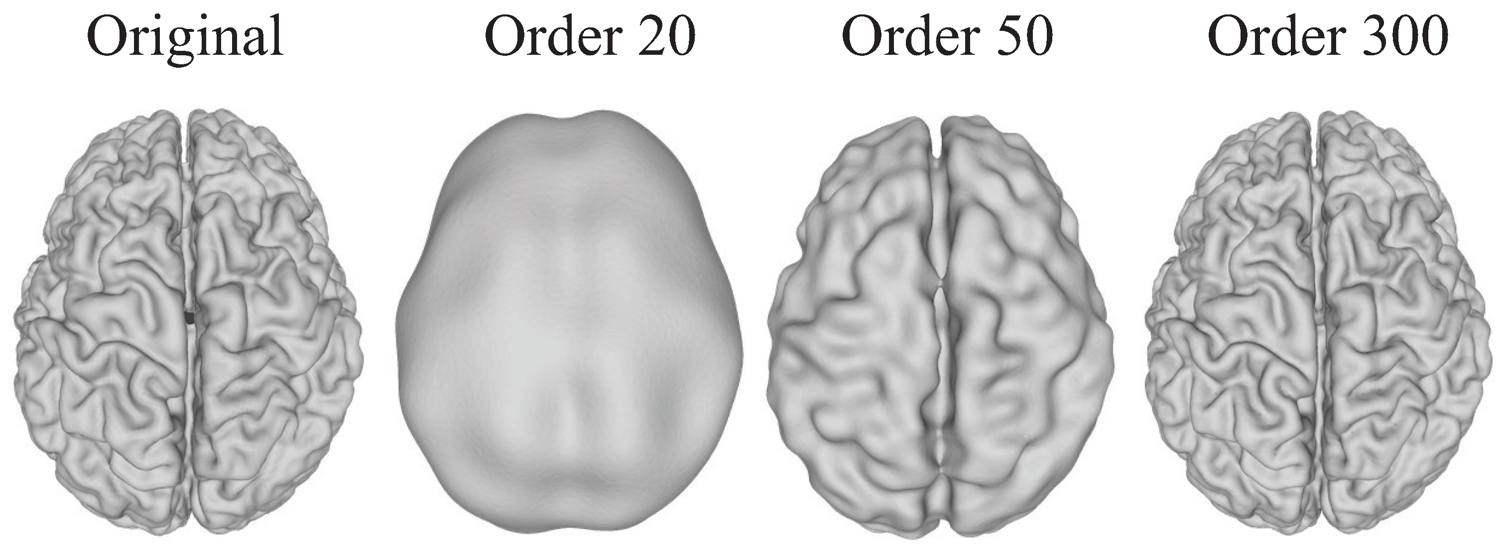
The final example, illustrated in Figure 11, corresponds to a brain surface. We use the brain surface data of one human subject from the Images and Data Archive of the USC Stevens Neuroimaging and Informatics Institute data set (accessed on 23 September 2022) (http://ida.loni.usc.edu). The brain surface obtained there is represented with a high quality oriented triangular mesh of genus zero, containing 65,538 vertices and 131,072 triangles. We computed its Zernike moments using the finite precision algorithm with a tolerance of ${10}^{-8}$, up to order 300. We then reconstructed the shape of the brain with orders 20, 50, and 300. Sulci, the grooves, and gyri, the folds, make up the folded surface of the brain. As the surface area of the brain increases from the formation of those sulci, more functions are made possible. A smooth-surfaced brain is only able to grow to a certain extent. Therefore, neurobiologists focus on those surface features when they study a 3D image of a brain. As shown in Figure 11, reconstruction of the surface of a brain from Zernike moments of orders up 20 only provides the general shape of this surface, with all sulci being smoothed out. The full geometry of those sulci, as observed in the original surface, is only restored with high orders moments are considered for the reconstruction, as illustrated in Figure 11 with $N=300$.

All examples shown above highlight the same conclusions: at low order, up to $N=50$, the Zernike moments only capture the global features of a shape. Order 50 is usually the limit to which Zernike moments can be computed for a shape represented by triangular meshes. The new algorithms presented in the paper allow for computing Zernike moments at much higher order. With $N=300$, we observe reconstructed meshes that capture the local features of the original shapes.

6.5. Computational Complexity for Geometric Moments and 3D Zernike Moments

The algorithm (Algorithm 2) introduced in Section 3 for the exact computation of the Zernike moments of a shape represented by a triangular mesh of its boundary is of order $O(M\times N^5)$ where M is the number of facets in the surface mesh, and N is the maximum order considered. The linear complexity with respect to the total number of facets coincides with the complexity of discrete algorithms that approximate the moments by applying a summation over the 3D image grid instead of computing an integral (considering constant value for the function over each grid cell). The second algorithm (Algorithm 3), which computes the Zernike moments with a finite precision is also of order M with respect to the number of facets.

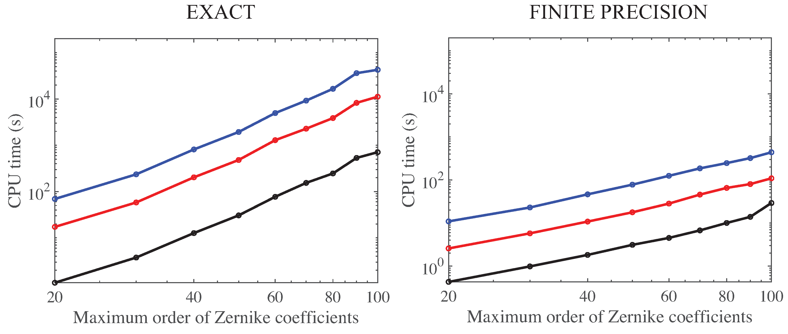
We implemented the two algorithms in a C++ program, Shape2Zernike, using double precision float arithmetics and tested their computational complexities on the simple case of a discrete sphere with radius 0.75, centered on the origin. We computed the Zernike moments for this sphere up to order 100 for the exact algorithm and for the finite precision algorithm, with the boundary of the sphere being represented with meshes with up to 1.3 million triangles. The experiments were run on an AMD Ryzen Threadripper PRO 3975WX processor with 193 GB of memory; each calculation was run as a single thread. Results are shown in Figure 12 and Figure 13.

The running time for the exact algorithm is found to be strictly linear with respect to the number of triangles in the mesh, as expected. The finite precision algorithm deviates from the linearity for meshes with small number of meshes. This is not unexpected. Indeed, the triangles of such meshes have larger surface area, requiring higher quadrature strengths for computing accurately the Zernike moments (see Figure 4). The finite precision algorithm remains significantly faster than the exact algorithm.

Similar trends are observed as we analyze the running time with respect to the maximum order of the Zernike moments (Figure 13). The apparent complexity of the exact algorithm with respect to the maximum order N of the Zernike moments are $O\left(N^{4.2}\right)$, different from the theoretical order $O\left(N^5\right)$. This can be understood as follows. For a given facet in the mesh, we sum the $g_{nl}^m$ over $O\left(N^2\right)$ points (i.e., the number of points needed for the strength of the quadrature that provides an exact integration on the facet). Computations of the $g_{nl}^m$ for each point proceed in two main steps. First, we need to compute the integrals $Q_{nl}$ and the spherical harmonics $Y_l^m$, both of complexity $O\left(N^2\right)$, and second, we need to assemble the $g_{nl}^m$ from those numbers. The second step is order $O\left(N^3\right)$, corresponding to the number of moments. Computing one $Q_{nl}$ or one $Y_l^m$ is significantly slower than assembling one $g_{nl}^m$, however. For small enough N the two steps take similar computing times. Hence at small N the apparent complexity is close to $O\left(N^4\right)$. At larger values of N (i.e., $N\gg 100$), the $O\left(N^5\right)$ complexity would be recovered. This situation does not occur as the maximum strength of the quadratures on a facet is 101, i.e., corresponds to N at most 100.

The apparent complexity of the finite algorithm is significantly better, of order $O\left(N^{2.4}\right)$. To understand the differences with the theoretical complexity of $O\left(N^5\right)$, we need to remember Figure 4. The actual strength of the quadrature needed to compute Zernike moments with a very small error ($TOL<{10}^{-8}$) is much smaller than the exact strength, especially for triangles with small areas. The spheres considered in our tests have more than 20,000 facets, all scaled so that the sphere is with radius 0.75. We found that for nearly all those triangles, the actual maximum strength was constant at the value 7, corresponding to only 13 points in the quadrature. This leads to a significant speedup of the algorithm. We note that this is the complexity expected in practical use of the algorithms, as shapes represented with triangular meshes are usually characterized by a large number of triangles, and those triangles have small areas when the shape is scaled to fit in the unit ball.

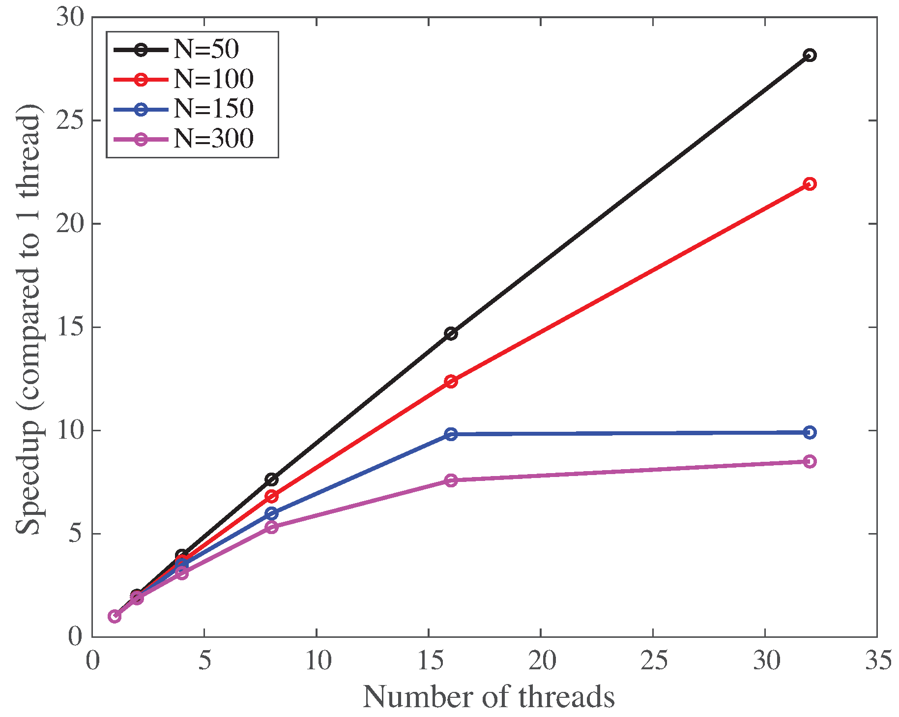
The algorithm maintains the independence of the contribution from each facet to the moments of the whole shape. This allows for an easy parallelization, which we implemented using POSIX threads. We tested the parallel version of Shape2Zernike on a Linux server, with Xeon Platinum 8168 CPU at 2.7 GHz with 96 cores and 396 GB of memory. The apparent speedups observed are reported in Figure 14. The calculations were performed on the gargoyle (see above), represented by a mesh with 100,000 triangles, for four maximum moment orders. The speedup factors were derived as an average over five independent runs, to minimize spurious fluctuations. For maximum orders up to $N=100$, the speedup remains fairly linear over the whole range of cores requested by the program. For a maximum order of $N=150$, a saturation appears, and the largest speedup factor is 8 for 16 cores used by the program. For a maximum order $N=300$, the same saturation occurs, and the maximum speedup factor is only 8, independent of the number of threads. We believe that the saturation effect observed is related to cache thrashing issues on each core, as the total storage required for large N values becomes important (a maximum order of 150 represents a total of 2,306,676 moments to be computed).

7. Conclusions

We have proposed two new algorithms for the computation of the homogeneous Zernike moments of a solid shape from a triangular mesh representing its boundary. Many algorithms have been proposed for computing such Zernike moments of a shape. Most of these methods usually proceed in two steps, namely computing the geometric moments of the shape first, and then expressing the Zernike moments as linear combinations of those moments. We have showed that this approach works well if the maximum order of the moments is small but fails for large order, due to numerical stability issues associated with computing the Zernike moments from the geometric moments. The new algorithms we propose circumvent this problem by computing directly from the shape. They rely on the analytical integration of the moments on tetrahedra defined by the surface triangles and a central point and on a set of novel recurrent relationships between the corresponding integrals. The first algorithm is exact. performing the computation of integrals over the triangles using quadratures of appropriate order. This algorithm, however, is mostly of academic interest due to its limitations. it requires quadrature rules with large strengths. Such rules include large number of sampling points, leading to an overall time complexity $O(M\times N^5)$, making it impractical. Quadrature rules, however, are known to converge fast. As such, it is not necessary to go to the maximum strength that is required for an exact computation. The second algorithm implements this idea. We have shown that it is fast, accurate, and allows for computations of moments of very high orders. We have shown also that this program can be easily parallelized, based on the independence of the contribution of each triangle in the boundary mesh. We did note however that as the number of moments that are computed increase, the memory requirement for each thread increases, leading to saturation effects in the parallelization speedup factor. This limitation related to memory would hinder a naive implementation of this algorithm on GPU. We are currently working on solutions to this problem. The free software implementing these algorithms is available at (accessed on 23 September 2022) (https://github.com/jerhoud).

References

- Zelditch, M.; Swiderski, D.; Sheets, H. Geometric Morphometrics for Biologists. A Primer; Elsevier: Amsterdam, The Netherlands; Academic Press: London, UK, 2012. [Google Scholar]
- Peng, H. Bioimage informatics: A new area of engineering biology. Bioinformatics 2008, 24, 1827–1836. [Google Scholar] [CrossRef] [PubMed] [Green Version]
- Khairy, K.; Howard, J. Spherical harmonics-based parametric deconvolution of 3D surface images using bending energy minimizations. Med. Image Anal. 2008, 12, 217–227. [Google Scholar] [CrossRef] [PubMed]
- Shamir, L.; Delaney, J.; Orlov, N.; Eckley, D.; Goldberg, I. Pattern recognition software and techniques for biological image analysis. PLoS Comput. Biol. 2010, 6, e1000974. [Google Scholar] [CrossRef] [PubMed] [Green Version]
- Toomre, D.; Bewersdof, J. A new wave of cellular imaging. Annu. Rev. Cell. Dev. Biol. 2010, 26, 285–314. [Google Scholar] [CrossRef] [PubMed] [Green Version]
- Thompson, D. On Growth and Form; University Press: Cambridge, UK, 1917. [Google Scholar]
- Hu, M. Visual pattern recognition by moment invariants. IRE Trans. Infor. Theory 1962, 8, 179–187. [Google Scholar]
- Teague, M. Image analysis via the general theory of moments. J. Opt. Soc. Amer. 1980, 70, 920–930. [Google Scholar] [CrossRef]
- Teh, C.; Chin, R. On image analysis by the methods of moments. IEEE Trans. Pattern Anal. Mach. Intell. 1988, 10, 496–513. [Google Scholar] [CrossRef]
- Prokop, R.; Reeves, A. A survey of moment-based techniques for unoccluded object representation and recognition. Graph. Model. Image Process. 1992, 54, 438–460. [Google Scholar] [CrossRef] [Green Version]
- Hobson, E. The Theory of Spherical and Ellipsoidal Harmonics; Chelsea Co.: New York, NY, USA, 1955. [Google Scholar]
- Byerly, W.E. An Elementary Treatise on Fourier’s Series, and Spherical, Cylindrical, and Ellipsoidal Harmonics, with Applications to Problems in Mathematical Physics. In Proceedings of the Spherical Harmonics; Dover: New York, NY, USA, 1959; pp. 195–218. [Google Scholar]
- Kazhdan, M.; Funkhouser, T.; Rusinkiewicz, S. Rotation invariant spherical harmonic representation of 3D shape descriptors. In Proceedings of the Eurographics Symposium on Geometry Processing, Aachen, Germany, 23–25 June 2003. [Google Scholar]
- Medyukhina, A.; Blickensdorf, M.; Cseresnyés, Z.; Ruef, N.; Stein, J.V.; Figge, M.T. Dynamic spherical harmonics approach for shape classification of migrating cells. Sci. Rep. 2020, 10, 6072. [Google Scholar] [CrossRef] [Green Version]
- Zernike, F. Beugungstheorie des Schneidenver-fahrens und seiner verbesserten Form, der Phasenkontrastmethode. Physica 1934, 1, 689–704. [Google Scholar] [CrossRef]
- Nguyen, T.; Pradeep, S.; Judson-Torres, R.; Reed, J.; Teitell, M.; Zangle, T. Quantitative Phase Imaging: Recent Advances and Expanding Potential in Biomedicine. ACS Nano 2022, 16, 11516–11544. [Google Scholar] [CrossRef] [PubMed]
- Tahmasbi, A.; Saki, F.; Shokouhi, S. Classification of begnin anf malignant masses based on Zernike moments. Comput. Biol. Med. 2011, 41, 726–735. [Google Scholar] [CrossRef] [PubMed]
- Boland, M.; Murphy, R. A neural network classifier capable of recognizing the patterns of all major subcellular structures in fluorescence microscope images of HeLa cells. Bioinformatics 2001, 17, 1213–1223. [Google Scholar] [CrossRef] [PubMed] [Green Version]
- Alizadeh, E.; Lyons, S.; Castle, J.; Prasad, A. Measuring systematic changes in invasive cancer cell shape using Zernike moments. Integr. Biol. 2016, 8, 1183–1193. [Google Scholar] [CrossRef] [PubMed]
- Toharia, P.; Robles, O.D.; Rodríguez, Á.; Pastor, L. A study of Zernike invariants for content-based image retrieval. In Proceedings of the Pacific-Rim Symposium on Image and Video Technology; Springer: Berlin/Heidelberg, Germany, 2007; pp. 944–957. [Google Scholar]
- Canterakis, N. 3D Zernike moments and Zernike affine invariants for 3D image analysis and recognition. In Proceedings of the 11th Scandinavian Conference on Image Analysis, Kangerlusssuaq, Greenland, 7–11 June 1999. [Google Scholar]
- Novotni, M.; Klein, R. 3D Zernike descriptors for content based shape retrieval. In Proceedings of the ACM Symposium on Solid and Physical Modeling, Seattle, WA, USA, 16–20 June 2003. [Google Scholar]
- Novotni, M.; Klein, R. Shape retrieval using 3D Zernike descriptors. Comput. Aided Des. 2004, 36, 1047–1062. [Google Scholar] [CrossRef]
- Wang, K.; Zhu, T.; Gao, Y.; Wang, J. Efficient terrain matching with 3-D Zernike moments. IEEE Trans. Aerosp. Elec. Sys. 2018, 55, 226–235. [Google Scholar] [CrossRef]
- Ma, B.; Zhang, Y.; Tian, S. Building Reconstruction Using Three-Dimensional Zernike Moments in Digital Surface Model. In Proceedings of the 2018 IEEE International Geoscience and Remote Sensing Symposium, Valencia, Spain, 22–27 July 2018. [Google Scholar]
- Capalbo, V.; De Petris, M.; De Luca, F.; Cui, W.; Yepes, G.; Knebe, A.; Rasia, E. The Three Hundred project: Quest of clusters of galaxies morphology and dynamical state through Zernike polynomials. Mon. Not. R. Astron. Soc. 2021, 503, 6155–6169. [Google Scholar] [CrossRef]
- Sael, L.; Li, B.; La, D.; Fang, Y.; Ramani, K.; Rustamov, R.; Kihara, D. Fast protein tertiary structure retrieval based on global surface shape similarity. Proteins Struct. Func. Bioinfo. 2008, 72, 1259–1273. [Google Scholar] [CrossRef]
- Venkatraman, V.; Sael, L.; Kihara, D. Potential for protein surface shape analysis using spherical harmonics and 3D Zernike descriptors. Cell. Biochem. Biophys. 2009, 54, 23–32. [Google Scholar] [CrossRef]
- Ljung, F.; André, I. ZEAL: Protein structure alignment based on shape similarity. Bioinformatics 2021, 37, 2874–2881. [Google Scholar] [CrossRef]
- Guzenko, D.; Burley, S.; Duarte, J. Real time structural search of the Protein Data Bank. PLoS Comput. Biol. 2020, 16, e1007970. [Google Scholar] [CrossRef]
- Burley, S.; Bhikadiya, C.; Bi, C.; Bittrich, S.; Chen, L.; Crichlow, G.; Christie, C.; Dalenberg, K.; Di Costanzo, L.; Duarte, J.; et al. RCSB Protein Data Bank: Powerful new tools for exploring 3D structures of biological macromolecules for basic and applied research and education in fundamental biology, biomedicine, biotechnology, bioengineering and energy sciences. Nucl. Acids. Res. 2021, 49, D437–D451. [Google Scholar] [CrossRef] [PubMed]
- Berman, H.M.; Westbrook, J.; Feng, Z.; Gilliland, G.; Bhat, T.N.; Weissig, H.; Shindyalov, I.; Bourne, P. The Protein Data Bank. Nucl. Acids. Res. 2000, 28, 235–242. [Google Scholar] [CrossRef] [PubMed] [Green Version]
- Aderinwale, T.; Bharadwaj, V.; Christoffer, C.; Terashi, G.; Zhang, Z.; Jahandideh, R.; Kagaya, Y.; Kihara, D. Real-time structure search and structure classification for AlphaFold protein models. Commun. Biol. 2022, 5, 1–12. [Google Scholar] [CrossRef] [PubMed]
- Senior, A.; Evans, R.; Jumper, J.; Kirkpatrick, J.; Sifre, L.; Green, T.; Qin, C.; Žídek, A.; Nelson, A.; Bridgland, A.; et al. Improved protein structure prediction using potentials from deep learning. Nature 2020, 577, 706–710. [Google Scholar] [CrossRef]
- Jumper, J.; Evans, R.; Pritzel, A.; Green, T.; Figurnov, M.; Ronneberger, O.; Tunyasuvunakool, K.; Bates, R.; Žídek, A.; Potapenko, A.; et al. Highly accurate protein structure prediction with AlphaFold. Nature 2021, 596, 583–589. [Google Scholar] [CrossRef]
- Desantis, F.; Miotto, M.; Di Rienzo, L.; Milanetti, E.; Ruocco, G. Spatial organization of hydrophobic and charged residues affects protein thermal stability and binding affinity. Sci. Rep. 2022, 12, 12087. [Google Scholar] [CrossRef]
- Venkatraman, V.; Yang, Y.; Sael, L.; Kihara, D. Protein-protein docking using region-based 3D Zernike descriptors. BMC Bioinform. 2009, 10, 407. [Google Scholar] [CrossRef] [Green Version]
- Christoffer, C.; Chen, S.; Bharadwaj, V.; Aderinwale, T.; Kumar, V.; Hormati, M.; Kihara, D. LZerD webserver for pairwise and multiple protein–protein docking. Nucl. Acids. Res. 2021, 49, W359–W365. [Google Scholar] [CrossRef]
- Daberdaku, S.; Ferrari, C. Exploring the potential of 3D Zernike descriptors and SVM for protein–protein interface prediction. BMC Bioinform. 2018, 19, 35. [Google Scholar] [CrossRef]
- Daberdaku, S.; Ferrari, C. Antibody interface prediction with 3D Zernike descriptors and SVM. Bioinformatics 2019, 35, 1870–1876. [Google Scholar] [CrossRef]
- Di Rienzo, L.; Milanetti, E.; Alba, J.; D’Abramo, M. Quantitative characterization of binding pockets and binding complementarity by means of Zernike descriptors. J. Chem. Inform. Model. 2020, 60, 1390–1398. [Google Scholar] [CrossRef]
- Milanetti, E.; Miotto, M.; Di Rienzo, L.; Monti, M.; Gosti, G.; Ruocco, G. 2D Zernike polynomial expansion: Finding the protein–protein binding regions. Comput. Struct. Biotechnol. J. 2021, 19, 29–36. [Google Scholar] [CrossRef] [PubMed]
- Di Rienzo, L.; De Flaviis, L.; Ruocco, G.; Folli, V.; Milanetti, E. Binding site identification of G protein-coupled receptors through a 3D Zernike polynomials-based method: Application to C. elegans olfactory receptors. J. Comput. Aided Molec. Des. 2022, 36, 11–24. [Google Scholar] [CrossRef] [PubMed]
- Memmolo, P.; Pirone, D.; Sirico, D.; Miccio, L.; Bianco, V.; Ayoub, A.; Psaltis, D.; Ferraro, P. Single-cell phase-contrast tomograms data encoded by 3D Zernike descriptors. arXiv 2022, arXiv:2207.04854. [Google Scholar]
- Hosny, K.; Hafez, M. An algorithm for fast computation of 3D Zernike moments for volumetric images. Math. Probl. Eng. 2012, 2012, 353406. [Google Scholar] [CrossRef] [Green Version]
- Berjón, D.; Arnaldo, S.; Morán, F. A parallel implementation of 3D Zernike moment analysis. In Proceedings of the Parallel Processing for Imaging Applications, San Francisco, CA, USA, 24–25 January 2011; SPIE: Bellingham, WA, USA, 2011; Volume 7872, pp. 83–89. [Google Scholar]
- De Araújo, B.; Lopes, D.; Jepp, P.; Jorge, J.; Wyvill, B. A survey on implicit surface polygonization. ACM Comput. Surv. (CSUR) 2015, 47, 1–39. [Google Scholar] [CrossRef]
- Lorensen, W.; Cline, H. Marching cubes: A high resolution 3D surface construction algorithm. ACM Siggraph Comput. Graph. 1987, 21, 163–169. [Google Scholar] [CrossRef]
- Doi, A.; Koide, A. An efficient method of triangulating equi-valued surfaces by using tetrahedral cells. IEICE Trans. Infor. Sys. 1991, 74, 214–224. [Google Scholar]
- Treece, G.; Prager, R.; Gee, A. Regularised marching tetrahedra: Improved iso-surface extraction. Comput. Graph. 1999, 23, 583–598. [Google Scholar] [CrossRef]
- Lien, S.; Kajiya, J. Symbolic method for calculating the integral properties of arbitrary nonconvex polyhedra. IEEE Comput. Graph. Appl. 1984, 4, 35–41. [Google Scholar] [CrossRef]
- Pozo, J.; Villa-Uriol, M.C.; Frangi, A. Efficient 3D geometric and Zernike moments computation from unstructured surface meshes. IEEE Trans. Pattern Anal. Mach. Intell. 2011, 33, 471–484. [Google Scholar] [CrossRef] [PubMed]
- Koehl, P. Fast Recursive Computation of 3D Geometric Moments from Surface Meshes. IEEE Trans. Pattern Anal. Mach. Intell. 2012, 34, 2158–2163. [Google Scholar] [CrossRef] [PubMed]
- Deng, A.W.; Gwo, C.Y. A Stable Algorithm Computing High-Order 3D Zernike Moments and Shape Reconstructions. In Proceedings of the 2020 4th International Conference on Digital Signal Processing, Chengdu, China, 19–21 June 2020; Association for Computing Machinery: New York, NY, USA, 2020; pp. 38–42. [Google Scholar]
- Tough, R.J.A.; Stone, A.J. Properties of the regular and irregular solid harmonics. J. Phys. A 1977, 10, 1261–1269. [Google Scholar] [CrossRef]
- Mathar, R.J. Zernike basis to Cartesian transformations. arXiv 2008, arXiv:0809.2368. [Google Scholar] [CrossRef] [Green Version]
- Janssen, A. Generalized 3D Zernike functions for analytic construction of band-limited line-detecting wavelets. arXiv 2015, arXiv:1510.04837. [Google Scholar]
- Prata, A.; Rusch, W. Algorithm for computation of Zernike polynomials expansion coefficients. Appl. Opt. 1989, 28, 749–754. [Google Scholar] [CrossRef]
- Stroud, A. Approximate Calculation of Multiple Integrals; Prentice-Hall: Englewood Cliffs, NJ, USA, 1971. [Google Scholar]
- Xiao, H.; Gimbutas, Z. A numerical algorithm for the construction of efficient quadrature rules in two and higher dimensions. Comput. Math. Appl. 2010, 59, 663–676. [Google Scholar] [CrossRef] [Green Version]
- Zhang, L.; Cui, T.; Liu, H. A set of symmetric quadrature rules on triangles and tetrahedra. J. Comput. Math. 2009, 89–96. [Google Scholar]
- Witherden, F.; Vincent, P. On the identification of symmetric quadrature rules for finite element methods. Comput. Math. Appl. 2015, 69, 1232–1241. [Google Scholar] [CrossRef] [Green Version]
- Wolfram Research Inc. Mathematica, Version 13.1; Wolfram Research: Champaign, IL, USA, 2022. [Google Scholar]
- Cignoni, P.; Callieri, M.; Corsini, M.; Dellepiane, M.; Ganovelli, F.; Ranzuglia, G. MeshLab: An Open-Source Mesh Processing Tool. In Proceedings of the Eurographics Italian Chapter Conference; Scarano, V., De Chiara, R., Erra, U., Eds.; The Eurographics Association: Saarbrücken, Germany, 2008. [Google Scholar]
- Cheng, H.; Shi, X. Guaranteed Quality Triangulation of Molecular Skin Surfaces. In Proceedings of the IEEE Visualization, Austin, TX, USA, 10–15 October 2004; pp. 481–488. [Google Scholar]
- Cheng, H.; Shi, X. Quality Mesh Generation for Molecular Skin Surfaces Using Restricted Union of Balls. In Proceedings of the IEEE Visualization, Minneapolis, MN, USA, 23–28 October 2005; pp. 399–405. [Google Scholar]
- Chou, J.; Li, S.; Klee, C.; Bax, A. Solution structure of Ca(2+)-calmodulin reveals flexible hand-like properties of its domains. Nature Struct. Biol. 2001, 8, 990–997. [Google Scholar] [CrossRef] [PubMed]
- Edelsbrunner, H. Deformable Smooth Surface Design. Discret. Comput. Geom. 1999, 21, 87–115. [Google Scholar] [CrossRef] [Green Version]
- Alber, T.; Banner, D.; Bloomer, A.; Petsko, G.; Phillips, D.; Rivers, P.; Wilson, I. On the three-dimensional structure and catalytic mechanism of triose phosphate isomerase. Philos. Trans. R. Soc. Lond. B Biol. Sci. 1981, 293, 159–171. [Google Scholar] [PubMed]
- Olver, F.W.J.; Olde Daalhuis, A.B.; Lozier, D.W.; Schneider, B.I.; Boisvert, R.F.; Clark, C.W.; Miller, B.R.; Saunders, B.V.; Cohl, H.S.; McClain, M.A. (Eds.) NIST Digital Library of Mathematical Functions. Available online: https://link.springer.com/article/10.1023/A:1022915830921 (accessed on 23 September 2022).
Figure 1.
Instabilities in evaluating the radial polynomials. In panel (A), we show the values of as a function of r, based on a stable evaluation of the polynomial function (see text for details). In panel (B), we show the values of the coefficients , the monomial expansion of .
Figure 2.
Instabilities in evaluating the factors. We show the maxima (in blue) and minima (in red) for the for a given n, as a function of n.
Figure 3.
Parameterization of a tetrahedron. Let be a triangle in the surface mesh, and be the associated tetrahedron where 0 is the origin. Any point within with spherical coordinates is projected onto the triangle T to a new point . Note that is a function of and .
Figure 4.
The strength N of the quadrature rule needed to compute the Zernike moment associated with a triangle of the surface mesh representing a shape is plotted against the surface area of this triangle.
Figure 5.
Numerical stability of the computation of Zernike moments. We plot the ratio of the sum of the norms of the Zernike moments to the value of ; this ratio should converge to (see Equation (38)). We use three different programs, PK-double that implements the PK algorithm which is a computation of the Zernike moments from the geometric moments of the shape using double precision 0, PK-GMP that implements the same calculation using full arbitrary precision arithmetic, and Shape2Zernike based on Algorithm 3 of this study.
Figure 6.
Numerical stability of the exact algorithm when computing the Zernike moments of discrete spheres. We plot the error in the numerical Zernike moments compared to the reference exact Zernike moments for a sphere (computed with Equation (40)) as a function of the number of triangles in the mesh represented the discrete sphere.
Figure 7.
Accuracy of the computation of Zernike moments for a cube with 12 facets as a function of the order n. The reference values were computed symbolically using a symbolic algebra system. The approximate algorithm is indistinguishable from the exact one.
Figure 8.
Summation of the series in Equation (33) for n up to N with and 200 for a scaled sphere with radius of . The series converges to a straight line at value 1 between the origin and , and vanishes beyond. Note the presence of overshoots, similar to oscillations in truncated Fourier expansions. Those overshoots concentrate as N increases.
Figure 9.
Reconstruction of a gargoyle (top row), a statue (middle row), and of the head of an ogre from the Zernike moments computed from a triangle mesh representing their boundaries. We compare the reconstructions generated from three different maximum order N, , , and . The original shape is shown on the left. All figures were generated with MeshLab [64].
Figure 10.
Reconstruction of Calmodulin (top row), and TIM (bottom row) from the Zernike moments computed from a triangle mesh representing their boundaries. Calmodulin (PDB code 1CLL) is a human small calcium binding protein while TIM (PDB code 1TIM) is the chicken triose phosphate isomerase. Both proteins are represented as a union of balls, with each ball corresponding to an atom. The surface of this union of balls, triangulated with the program smesh [65,66], serves as input to the computation of the Zernike moments of their shapes. We compare the reconstructions generated from three different maximum order N, , , and . The original shape is shown on the left. All figures were generated with MeshLab [64].
Figure 11.
Reconstruction of the surface of a brain from the Zernike moments computed from a triangle mesh representing its boundary. We compare the reconstructions generated from three different maximum order N, , , and . The original brain surface is shown on the left. All figures were generated with MeshLab [64].
Figure 12.
CPU times required to compute the Zernike moments of a sphere as a function of the number of triangles in the meshes that represent this sphere. We compare the exact algorithm (left) with the finite precision algorithm (right), while the time complexity for the former is found to be strictly linear with respect to the number of triangles, it deviates from linearity for the latter. We observe the same behavior for different maximum order N (20, 50 and 100) at which the Zernike moments are computed.
Figure 13.
CPU times required to compute the Zernike moments of a sphere as a function of the maximum order N of those Zernike moments. We computed the Zernike moments for three discrete representations of the sphere, each given by a triangular mesh. The corresponding meshes include 20,480, 81,920 (black line), and 327,680 (red line) triangles, respectively. Linear fits to these curves give slopes of 4.2 for the exact algorithm and 2.4 for the finite algorithm, corresponding to apparent complexities of and for those two algorithms.
Figure 14.
CPU time required to compute the Zernike moments of the gargoyle The speedup in clock time is plotted against the number of CPU or threads used by the parallel version of the approximate algorithm, for different maximum order (50, 100, 150, and 300). The speedup is obtained as an average over 5 independent runs.
Publisher’s Note: MDPI stays neutral with regard to jurisdictional claims in published maps and institutional affiliations. |
© 2022 by the authors. Licensee MDPI, Basel, Switzerland. This article is an open access article distributed under the terms and conditions of the Creative Commons Attribution (CC BY) license (https://creativecommons.org/licenses/by/4.0/).
Share and Cite
MDPI and ACS Style
Houdayer, J.; Koehl, P. Stable Evaluation of 3D Zernike Moments for Surface Meshes. Algorithms 2022, 15, 406. https://doi.org/10.3390/a15110406
AMA Style
Houdayer J, Koehl P. Stable Evaluation of 3D Zernike Moments for Surface Meshes. Algorithms. 2022; 15(11):406. https://doi.org/10.3390/a15110406
Chicago/Turabian StyleHoudayer, Jérôme, and Patrice Koehl. 2022. "Stable Evaluation of 3D Zernike Moments for Surface Meshes" Algorithms 15, no. 11: 406. https://doi.org/10.3390/a15110406
Note that from the first issue of 2016, this journal uses article numbers instead of page numbers. See further details here.