1. Introduction
Colorectal cancer is the third most frequently detected type of cancer among men and the second among women [
1,
2]. According to WHO data, around 1.8 million new cases and more than 800,000 deaths are detected annually [
3]. Moreover, colorectal cancer is one of the most common causes of mortality [
4,
5]. Currently, histological image analysis is the standard for the clinical diagnosis of cancer [
6,
7].
The basis for cancer treatment is the morphological verification of the tumor process, based mainly on the material of an endoscopic biopsy of the colon. Pathoanatomic examination is a subjective process based on the recognition of various morphological structures on histological slides, and only specialists can deal with the problem. The limited number of available pathologists make it difficult to establish a system of reference studies of all biopsies. The problem can be substantially facilitated with computer technologies.
In recent years, artificial intelligence and deep learning [
8,
9,
10], in particular, have found wide application in different areas of medical research and medical imaging. Many studies are devoted to the X-ray [
11,
12] and MRI [
13,
14,
15,
16] image processing. Machine learning methods are used to analyze different types of data obtained with a colonoscopy, CT colonography, colon capsule endoscopy, endocytoscopy, and other techniques. The increasing amount of available digital histological images makes it possible to use machine learning methods to segment and classify cancer types [
17,
18].
Whole-slide imaging (WSI) provides extensive opportunities in this area using deep learning. This is a segmentation task, and WSIs have been shown to be segmented into the areas of healthy tissues and those containing cancer with high accuracy using convolutional neural networks (CNN) [
19] or autoencoders that include various CNNs [
20]. The scientists often consider the classification problem with only two classes—detection of malignant tissue in a given WSI fragment [
21]. J. Noorbakhsh et. al. showed that neural networks trained on images of some tissues are able to classify other tissues with high accuracy [
22]. To diagnose lymphoma, Bayesian neural networks achieved a quality of AUC = 0.99 [
23]. A. D Jones, et. al. compared the prediction quality of neural networks trained on PNG and JPG images for breast, colon, and prostate tissues and found that there were no statistically significant differences; therefore, it is possible to use JPG to reduce the training time and memory used [
24].
In [
25,
26], multi-class classification was performed with CNN, and cancerous tissues were detected and differentiated. For the same purposes, H. Ding et. al. [
27] used the fully convolutional network [
28]. In [
29], the network trained on WSI data was transferred for the analysis of MSI, and H. Chen et al. [
30] proposed a new loss function that allowed more efficient CNN training of CNN on WSI data.
Most works devoted to the use of neural networks for cancer diagnostics address the problem of binary classification between malignant and benign tissues. The use of neural networks to diagnose colorectal cancer is not so popular for other organs, such as the breast. For example, in the Scopus research database, there are 2850 studies for the query “deep learning” AND “Breast cancer”, while only 628 studies for the query “Deep learning” AND “colorectal cancer”.
In this work, we collected WSIs of colon tissue samples and trained CNN to classify them into six classes. To deal with WSI data, a training sample caching system was designed and implemented. Several classification approaches were compared: multi-class classification and one-vs-rest classification, and the one-cycle policy method was also used [
31] to configure training hyper-parameters.
2. Materials and Methods
2.1. WSIs Database
When labeling the images, we used the diagnostic criteria of the current edition (fifth) of the WHO classification of gastrointestinal tract tumors [
32]. Three GI pathologists, with at least 7 years of work experience, were responsible for performing the image segmentations on a commercial basis. Each pathologist was engaged in the segmentation of his set of WSIs. Upon completion, the head of the group of pathologists (Karnaukhov N.S.) checked the markup and corrected the labels he considered incorrect classification. In the case of any other pathologist discordance, he fixed the segmentation issues, being the most qualified specialist.
We selected the criteria describing the morphological structures characteristic of all types of benign and malignant tumors of the colon, according to WHO recommendations. A systematization of histological slides was conducted, with a discussion of various pathological processes. The classes of histological categories involved in the histological conclusion were formed, namely:
structures of normal colon glands (NG);
structures of serrated lesions (SDL);
structures of serrated lesions with dysplasia (SDH);
structures of hyperplastic polyp, microvesicular type (HPM);
structures of hyperplastic polyp, goblet-cell type (HPG);
structures of adenomatous polyp, low-grade dysplasia (APL);
structures of adenomatous polyp, high-grade dysplasia (APH);
structures of tubular adenoma (TA);
structures of villous adenoma (VA);
structures of glandular intraepithelial neoplasia, low-grade (INL);
structures of glandular intraepithelial neoplasia, high-grade (INH);
structures of well differentiated adenocarcinoma (AKG1);
structures of moderate differentiated adenocarcinoma (AKG2);
structures of poorly differentiated adenocarcinoma (AKG3);
structures of mucinous adenocarcinoma (MAK);
structures of signet-ring cell carcinoma (SRC);
structures of medullary adenocarcinoma (MC);
structures of undifferentiated carcinoma (AKG4);
Granulation tissue (GT).
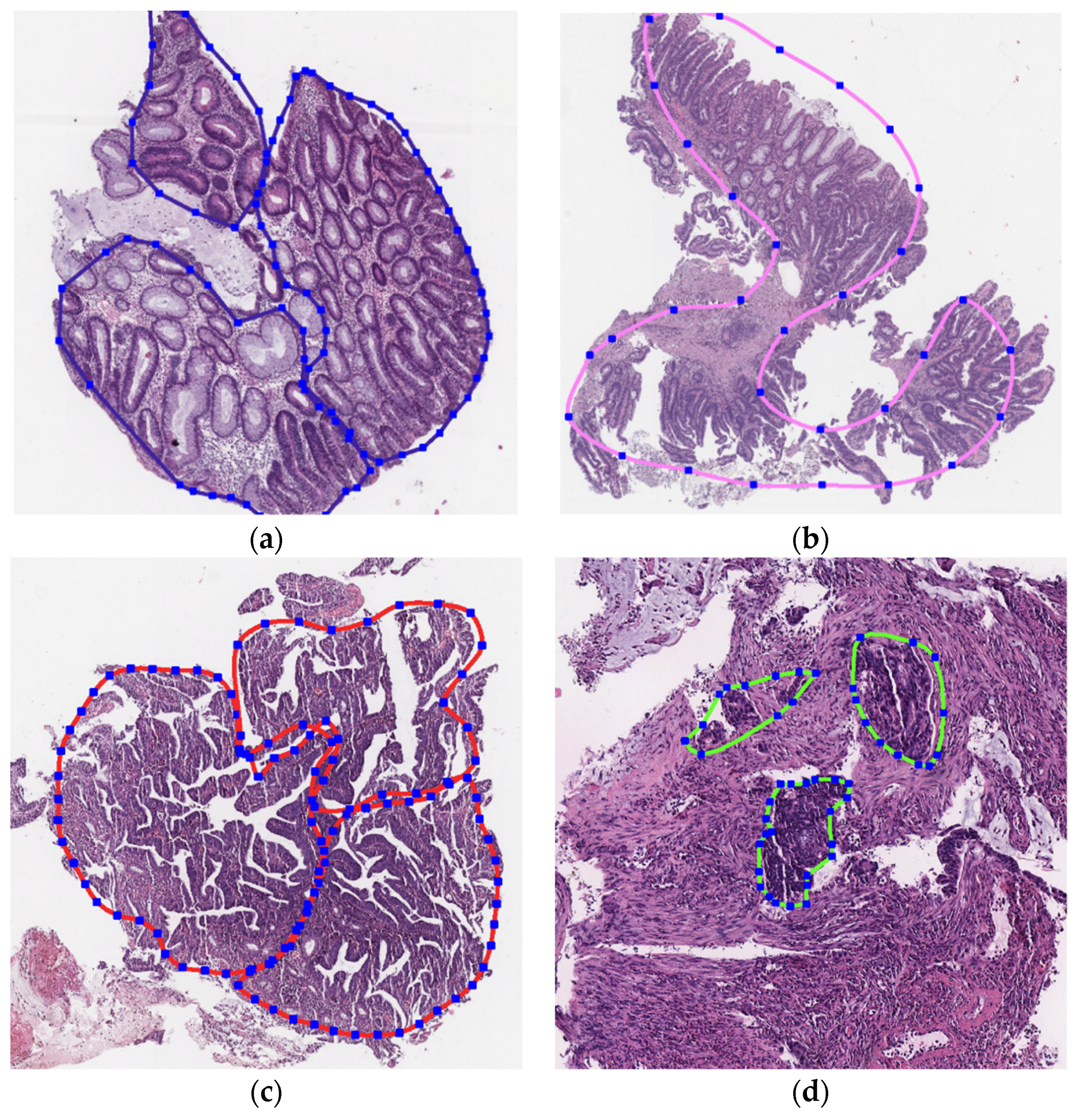
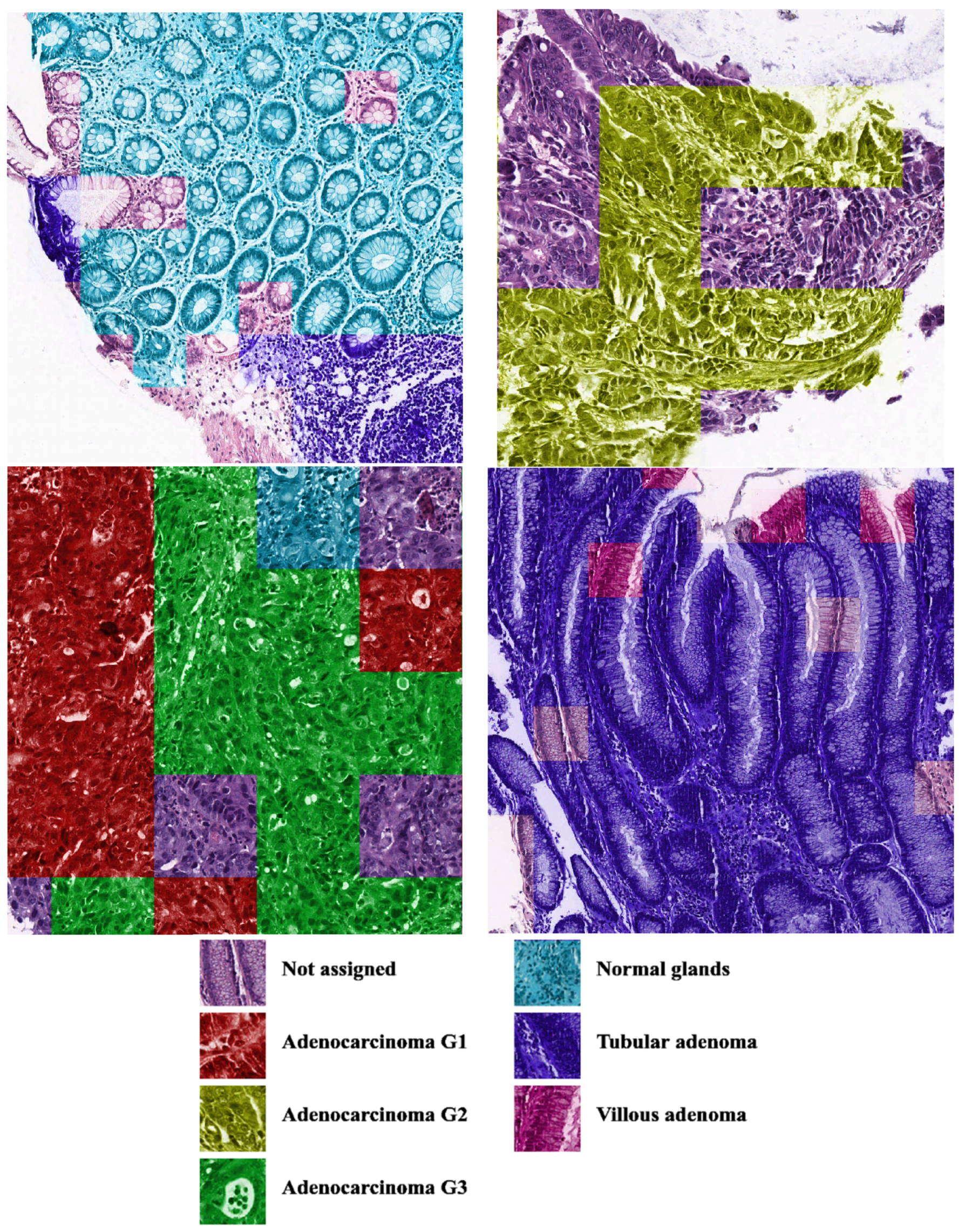
Histological samples from endoscopic colon biopsies were digitized (.svs) with a Leica Aperio AT2 scanning microscope, with a resolution of 0.50 µm/pixel. The scanned images were divided equally between 3 specialists. Each specialist labelled the histological structures with the ASAP software. Several representative examples are shown in
Figure 1.
Each labelled area was outlined with its own color. The pathologists tried to avoid fibrous tissue, artifacts from histological slides, and the white background falling into the labelled area. The borders of the labelled areas were not allowed to intersect.
Some classes of histological categories are based on the presence of several morphological structures, for example, tubulovillous adenoma. We did not consider mixed structures as separate classes because such mixtures were already identified in the output of machine learning classification. When the ML algorithm returned significant probabilities for several classes, the output was treated as a mixture of structure types.
We used the WHO classification of the gastrointestinal tract, 5th edition, but did not aim to train the algorithm to make a diagnosis. The main purpose of the study was implementing the automatic segmentation system so that pathologists can perform diagnoses faster. All slides were collected and processed at the National Medical Research Center of Oncology, Rostov-on-Don. The total number of WSIs was 1785.
2.2. WSIs Preprocessing
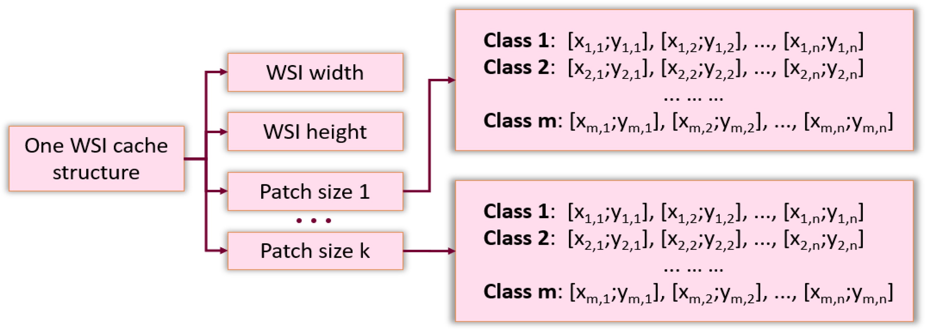
WSIs are multi-layered images combining histological slides with different magnifications. The WSIs were scanned with high resolution, and the size of the digitized slide was able to reach 80,000 × 60,000 pixels. Each individual image took up 80 MB to 1.5 GB of computer memory. Due to the large sizes of the source images, their direct use for CNN training was not possible. Therefore, we split the original images into small patches and used them for training and testing CNN, with the exception of uninformative patches (representing a white background or containing less than 50% of the total area with tissues).
Splitting WSIs into patches and saving them to a separate file was time consuming for a large database of images. This procedure had to be repeated when the size of the patch was modified. The caching system overcame these issues. This system was implemented in the form of an associative array, which for each WSI, stored metadata: image dimensions and lists of the coordinates of the patch in the source image for each class, depending on the desired size of the patch (see
Figure 2). Upon training and testing, the patches were read directly from the original WSI according to the desired size and the coordinates stored in the cache.
Only the normalizing and CLAHE (contrast limited adaptive histogram equalization) operations from Albumentations (a Python library for image augmentation) [
33] were used for patch preprocessing. Representative examples of patches before and after preprocessing are shown in
Table 1.
2.3. Approaches to the Problem Statement: Multi-Class and Multi-Label
The problem of classifying WSI patches can be solved by two approaches: multi-class and multi-label. The multi-class ML approach returns a normalized vector of class probabilities for a given object. The number of elements in the vector coincides with the number of classes, and their sum is equal to 1, which in probability theory, indicates that an object must belong to exactly one of the classes under consideration. On the contrary, the multi-label approach is applied to tasks where objects may belong to several classes at once or to none of them.
The multi-class approach has a significant drawback. If pathologists do not label all types of cells that may be found in the images, then an ML algorithm will fail in classifying cells beyond the labelled types. However, it is difficult to label all types of cells due to several reasons: (1) it is time consuming, (2) it is unclear which classes should be assigned for the cells not involved in the diagnosis or playing a secondary role, and (3) there are many intermediate classes combining the features of several “pure” classes. Therefore, we focused on selected classes that were particularly important for diagnosis from a pathologist’s point of view. We applied the algorithms to all areas of the images without exception, while many cell types were not included in the training set. The probability normalization at the output of a multi-class neural network would significantly overestimate the probabilities of classes for the areas with unlabeled types. The correct approach was to disable normalization and consider the task as a multi-label classification task.
From the point of view of the neural network structure, the multi-label classification differs from the multi-class one only by the normalization on the last layer. A neural network trained as a multi-label one will assign high probabilities only for classes from the training sample. The remaining objects will receive low probabilities for all classes and thus do not require the attention of a pathologist.
2.4. The Structure and Types of Neural Networks
The idea of transfer learning was used to classify WSI fragments [
34]. We used deep neural networks pre-trained on the ImageNet dataset as a basis and provided additional training on images from our WSI database to adapt these networks for a specific task. ResNet deep convolutional neural networks [
35] and EfficientNet [
36] architectures were considered. The deep convolutional neural network is one of the most common architectures used for image recognition and showed good results in the ImageNet competition. To solve our problem, we used the ResNet network with a different number of layers: 34, 50, 101, and 152. Some configurations of the EfficientNet networks had less parameters to be optimized (see
Table 2) and thus was able to be trained and implemented much faster than ResNet networks.
2.5. Training the Neural Network
This study focused on the 6 most common classes in the WSI fragments: normal glands (NG), adenocarcinoma G1 (AKG1), adenocarcinoma G2 (AKG2), adenocarcinoma G3 (AKG3), tubular adenoma (TA), and villous adenoma (VA). The “tubular” and “villous” classes only encompassed low- and high-grade adenomas and did not contain adenocarcinomas (as these classes could overlap). We selected these labels to make our work comparable with existing AI applications, namely the web platform cancercenter.ai, based on ICD-O 3 morphological codes.
Two strategies were used to solve the classification problem:
The neural networks for both classification problems were based on a common principle. They relied on a convolutional neural network for feature extraction. Three fully connected layers with the ReLU activation function that performed the classifier task were added to this CNN. A sigmoid activation function was applied to the network output.
For the task of 6-class classification, the outputs of the neural network did not readily correspond to the probabilities of the corresponding classes. A procedure was implemented to convert the output of a neural network to values characterizing the probabilities.
2.6. Converting Neural Network Outputs to Class Probabilities
Despite the presence of a softmax layer at the output of the multi-class neural network, the resulting outputs generally differed from the probabilities. In practice, it would be convenient to obtain the exact probabilities, for example, as an image with colored fragments when the neural network is confident in its classification with a given probability. To convert the outputs of the neural network to probabilities, we used the following algorithm.
Let us denote
—the part of the multi-class neural network that accepts an image patch x as input and returns the value
in the interval [0, 1]—as the degree of x matching class c. For each value t of
, we define a subset
of the training sample
, with the image
providing the value of the neural network
larger than the threshold t:
Then, the value
t of the neural network can be converted to the probability
of class c by calculating the accuracy of
in
:
where vertical lines
denote the cardinality of a set.
When training neural networks to binary one-vs-rest problems, the values obtained by applying the sigmoid to the network outputs were considered as the probability that a WSI patch belonged to the target class.
2.7. Training Neural Networks
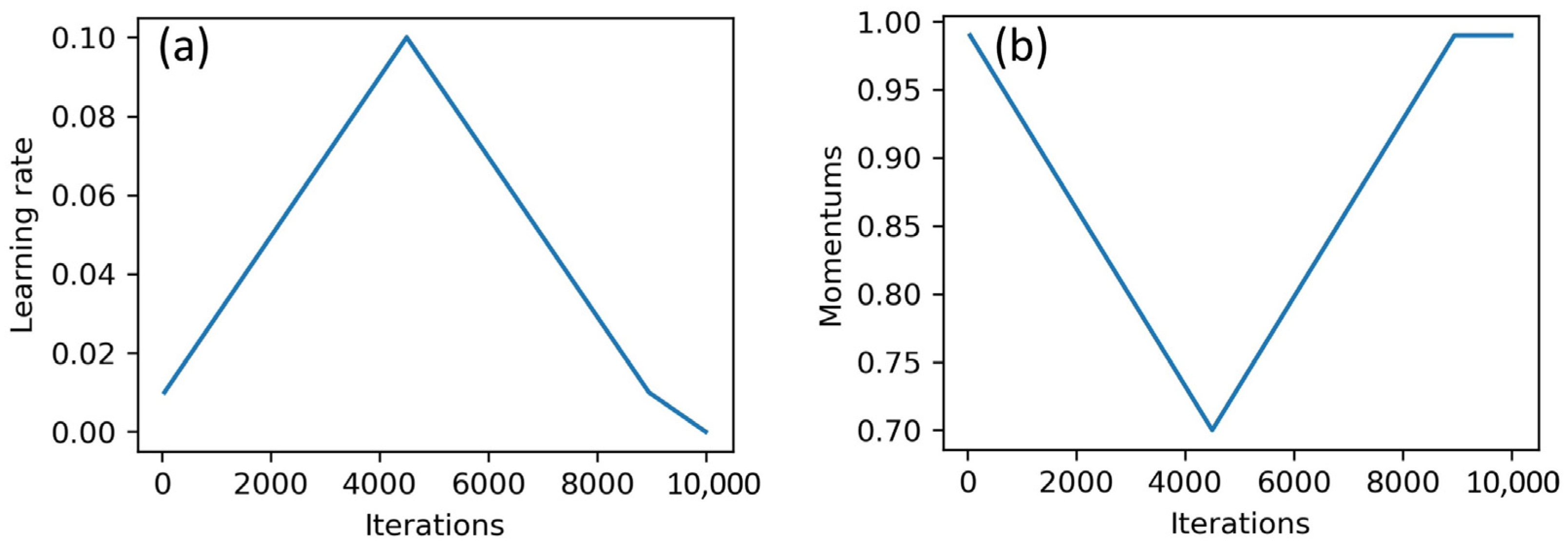
The process of training neural networks was carried out in two ways: classical approach and one-cycle policy. In the classical approach, the parameters of the neural network were optimized over several epochs of training by stochastic gradient descent (SGD), with fixed values of learning rate and momentum. When using the one-cycle policy, the neural network was trained in one epoch with the SGD method. In the training process, the values of the learning rate and momentum changed through a fixed number of training iterations. The training process was divided into three stages. The first two stages had the same length, and the final stage contained only a few iterations. The maximum value of the learning rate was set in a first step. The minimum value of the learning rate was usually set at 0.2 or 0.1 of the maximum value. At the first stage, the learning rate increased from the minimum to the maximum value. In the second stage, the opposite was true. For the third stage, 1/100 of the maximum value was usually taken. The values of the momentum decreased at the first stage and increased at the second and third stages (See
Figure 3).
This strategy to vary the parameters of the SGD optimizer was sort of a regularization and helped to avoid overfitting the network and train it much faster [
31]. Moreover, this approach worked much faster than the classical one, since neural networks in the process of such training achieved high performance in one training epoch.
The binary cross-entropy function was used as a loss function for training and the mean function for the reduction of outputs.
2.8. Evaluation. Train and Test Splitting
The objects of the neural network analysis were the small patches of complete WSIs. Therefore, a common mistake during the evaluation of the trained neural network was to split the set of patches into training and test parts of the sample without considering the WSIs these pieces were taken from. The patches of the same image had similar features: a color scheme, characteristics for a given place and direction of the cross section of cell structures, and a certain type of intercellular space. If some of these patches fell into the training sample of the neural network, the network would learn to recognize them, and the quality of the results on the test sample would be overestimated. However, the goal was to apply the neural network for patches of completely new images, parts of which had never been used during training. Therefore, the test would be valid if we split the training and test samples before splitting the WSIs into patches. This approach complicated the program code and introduced the problems associated with significantly different proportions of classes in the training and test sets of images. However, it allowed one to obtain an adequate quality criterion.
The entire sample of WSIs was split into train, validation, and test datasets in the ratio of 60%, 20%, and 20%, respectively. The number of source images and patches of different sizes is shown in the
Table 3.
Neural networks made more reliable predictions when trained with balanced data. Random oversampling was applied to the training sample to equalize the neural network capabilities for adjusting weights for different classes.
2.9. PR Curves and Their Normalization
WSI patches that were confidently classified by a neural network were of great interest. The PR curve enabled the assessment of the precision and the recall of the classification for different values of the degree of confidence. It was plotted for each class of image patches. We used the average area under the PR curves of all classes as an integral characteristic of the classification quality for all classes.
For each class included in the integral characteristic with the same weight, the proportion of patches in the test set should be the same. To ensure this, the undersampling technique was used. After randomly selecting sets of WSIs of the test set, we calculated the number of patches of each class, selected the smallest, and used this number to perform random undersampling in all other classes.
With this approach, all PR curves had (1; alpha) as their rightmost point, where alpha is the percentage of patches in the smallest class. Thus, the PR curves were normalized, and the effect of different classes on the integral metric was equalized.
3. Results
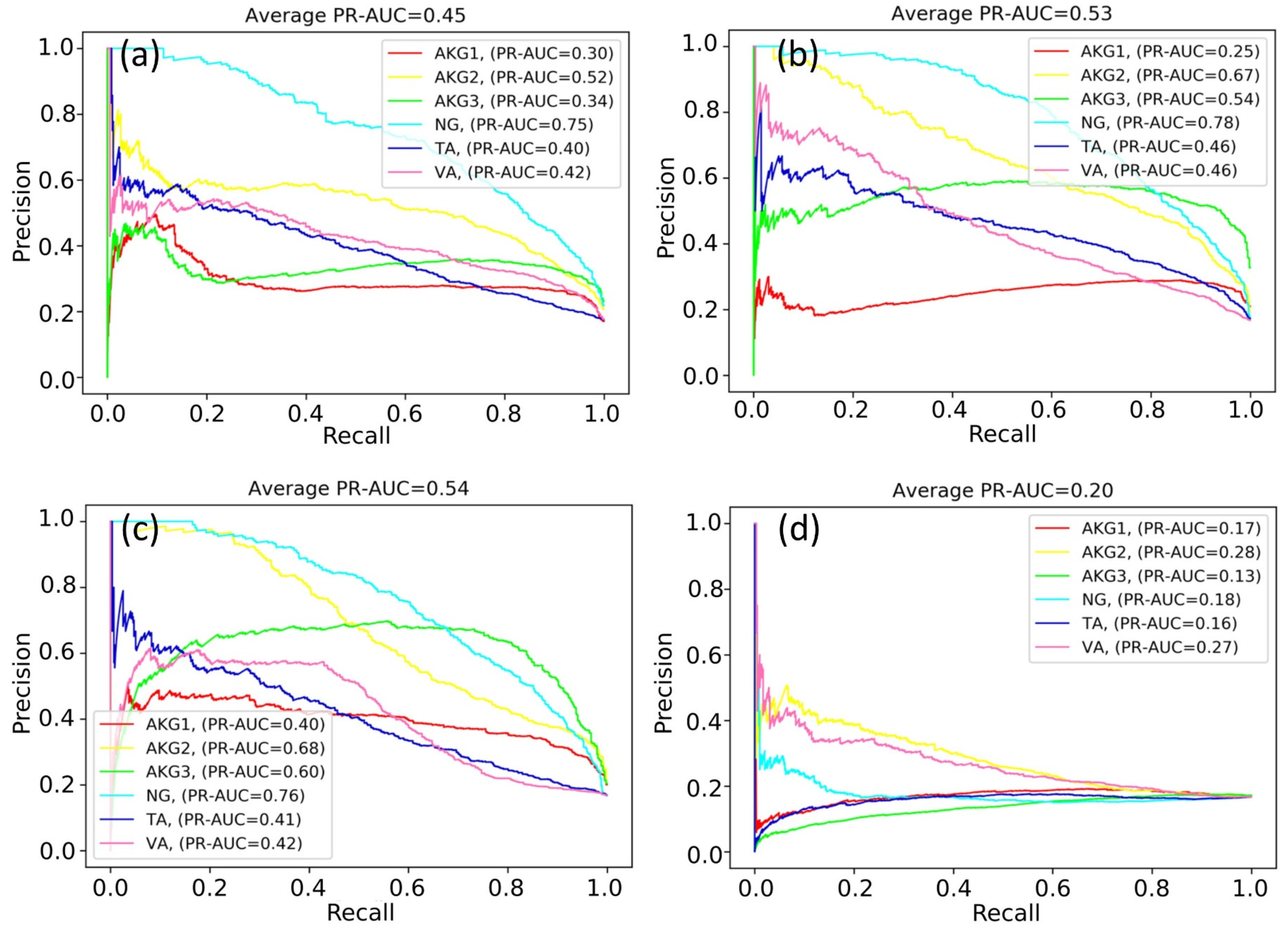
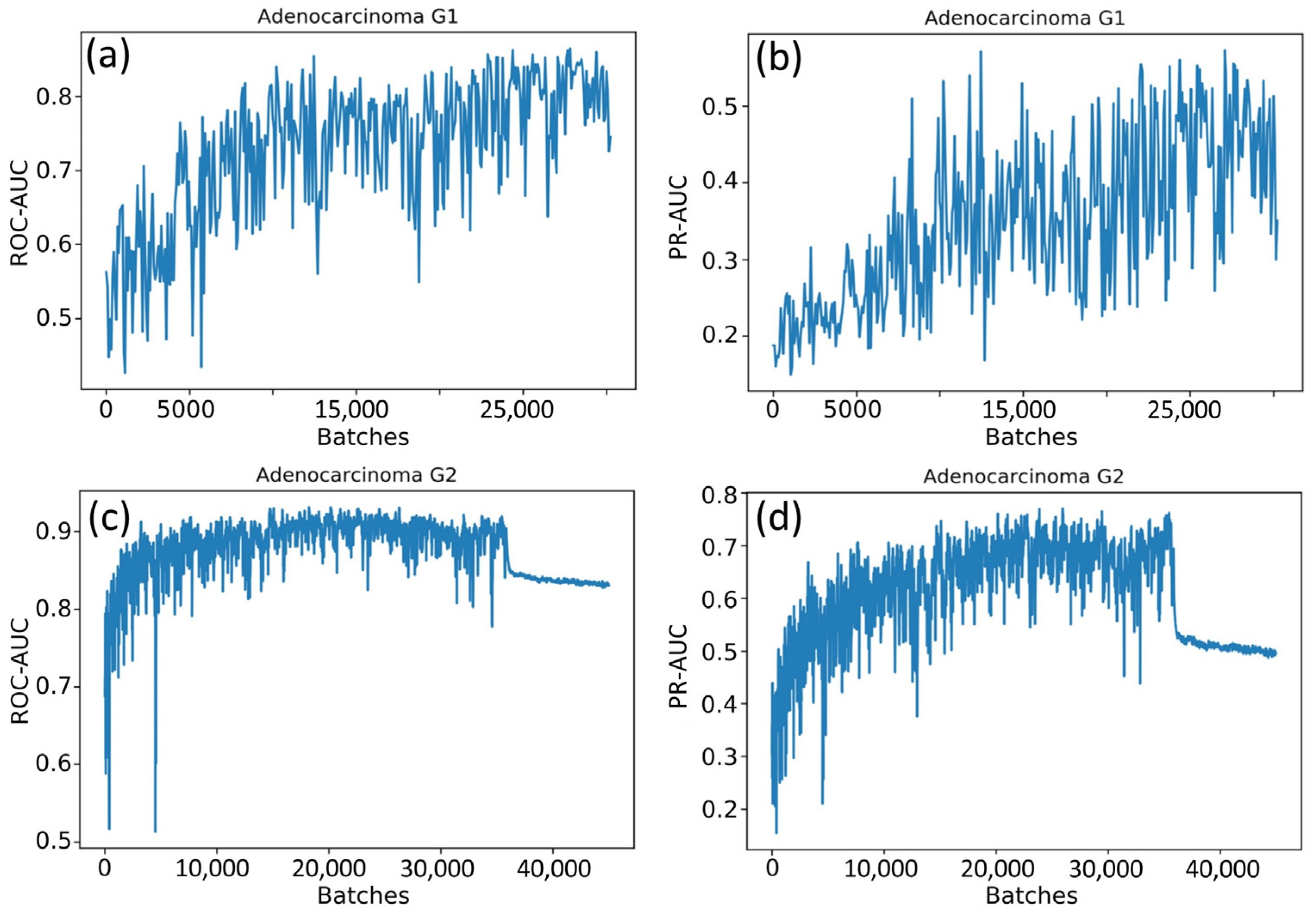
In the first experiment, we trained a single neural network to classify patches of a WSI into six classes. The neural network was trained according to the one-cycle policy. The quality of the prediction was evaluated with the PR-AUC value for each class during training.
Figure 4 shows the variations in PR-AUC graphs.
According to
Figure 4, the classification quality of some classes increased or fluctuated (NG and AKG2 classes), while the classification quality of other classes decreased (for example, TA and VA classes). As a result of many experiments, it was not possible to find out the optimal number of training iterations maximizing values of PR-AUC simultaneously for all classes.
At some point, the PR-AUC values decreased, indicating almost random predictions. This might be the consequence of extremely high values of neural network weights and indicate the exploding gradient problem. The problem arises due to the exponential growth of gradients in the training process, and in turn, the growth of the weights of the neural network to infinity.
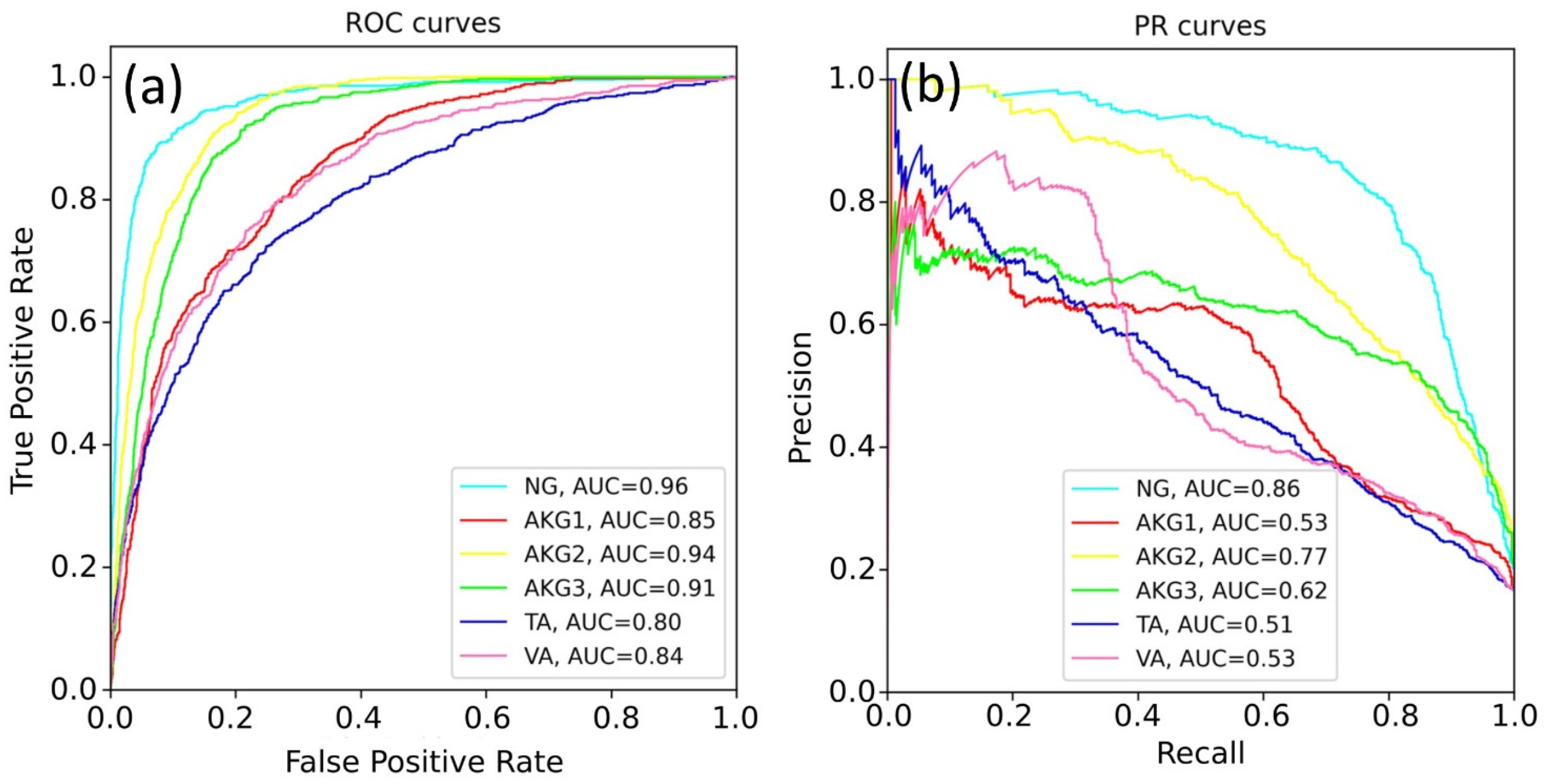
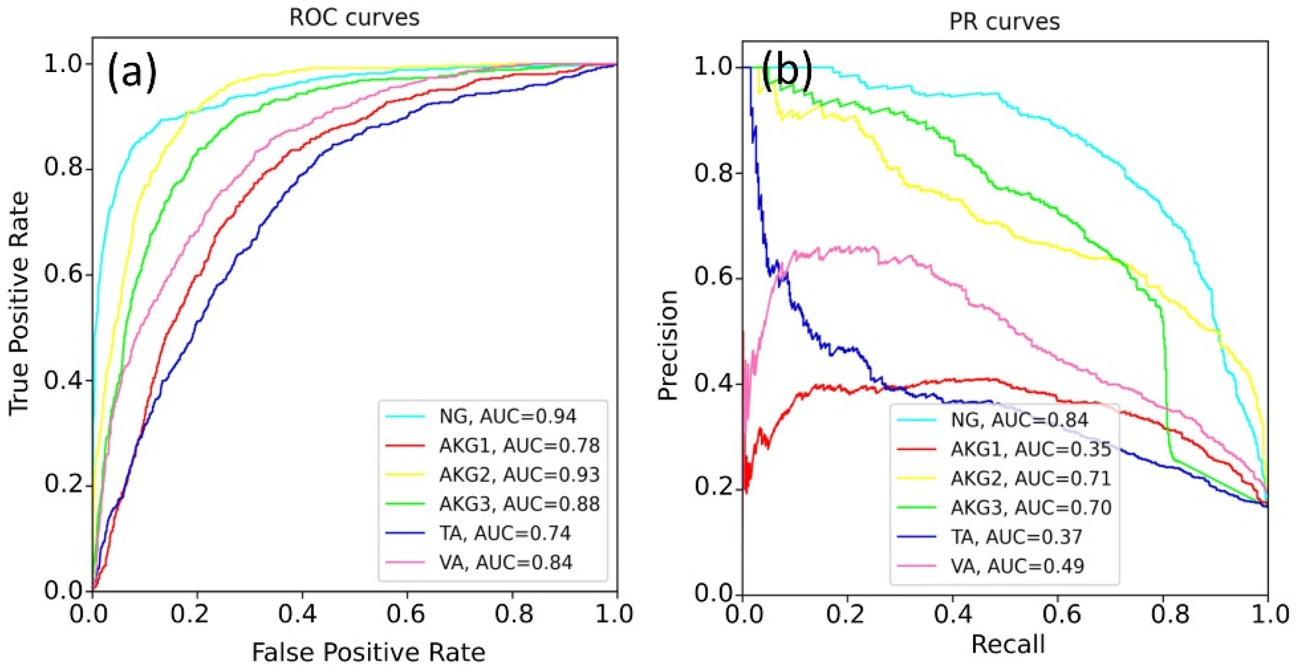
The weights of the network grew unequally for different classes. That is why we constructed six independent neural networks to solve the one-vs-rest binary classification problem. The classification quality in this case was evaluated with the accuracy, ROC-AUC, and PR-AUC metrics. Neural networks based on ResNet and EfficientNet architectures were compared, and the sizes of the WSI patches (224 × 224 and 500 × 500) were also varied. Selected results for EfficientNet-B4 are shown in
Figure 5.
The best results were obtained for the NG class. This can be explained by a variety of available images of this class and the lower specificity of healthy tissues. The rest models demonstrated a lower quality of classification, since pathological tissues may have similar features.
Table 4 shows the best prediction results for each class, according to the ROC-AUC and PR-AUC metrics. The EfficientNet-b4 model showed the best results for most tasks.
The problem of multi-label classification implies that it is the choice of a probability threshold to determine whether an object belongs to a certain class. Several other metrics can be applied in addition to ROC-AUC and PR-AUC, such as sensitivity, specificity, precision, F1 score, and negative predictive value (NPV). All of them directly depend on the value of the probability threshold.
Table 5 shows the values of these metrics for a threshold = 0.5 for both patch-level and WSI-level.
The CNN classification can be transferred to the real images.
Figure 8 shows the output of the software, where the colors of the patches correspond to class colors in
Figure 4,
Figure 6 and
Figure 7. The software painted the patches where predicted class probability was greater than 0.5.
As an output of our program, we received the probability (the value from 0 to 1) for each of the six tissue types that the patch belonged to. If all the probabilities were below the threshold, we did not assign any class to the patch. In this case, the patch may have belonged to the unknown class. When several classes had probabilities greater than the threshold, the prediction was «mixed»; that is, the patch consisted of several areas belonging to different tissue types. It would be inconvenient to analyze the result of the painted WSI if we used special markers for all mixed types. Such patches could be highlighted for the specialist; otherwise, we painted the mixed patches with the color of the most probable type, while the threshold could be chosen by the user.
4. Discussion
The development of new methods for diagnosing colorectal cancer burdens pathologists with the work of segmentation. Deep learning has been successfully applied in computational pathology in the past few years to automate this task. The computer program can process large amounts of WSI automatically without feeling fatigue, thus becoming a useful AI assistant for pathologists. The application of deep learning in the diagnosis of colorectal or other types of cancer has many advantages, such as the high speed of diagnosis. However, it has some limitations as well. Reliable identification of colon tumors (
Section 2.1) requires a similar amount of WSI for each type. This is quite difficult to provide, due to the rare occurrence of certain diseases. Even for a human specialist, the correct definition of the cancer is quite a difficult task. The problem of differentiation between six types of lesions solved in this work is more complex, compared to the common binary classification of histological images. This explains lower values of the area under ROC curves, compared to the most published works [
19,
24,
25,
29].
The closest results were obtained recently by Masayuki Tsuneki and Fahdi Kanavati [
37]. Using the database of 1799 WSI, they performed binary classification to detect the colorectal poorly differentiated adenocarcinoma. Using the same transfer learning, the authors managed to achieve a receiver operating characteristic curve-area under the curves of up to 0.95. A strict comparison of this result with our 0.91 is inappropriate, due to different database statistics, but a rough comparison is very useful. The test database of M.Tsuneki and F.Kanavati consists of 74 WSIs with a poorly differentiated ADC diagnosis, 404 moderately differentiated ADCs, 643 adenoma, and 678 non-neoplastic subsets. The authors focused on the problem of poorly differentiated ADC discrimination. This class diagnosis is rare and requires special treatment.
Due to the rarity of the poorly differentiated ADCs, our dataset contained only 21 such cases out of 1785 WSI. As we split the whole database into train 60%, validation 20%, and test 20% parts, the last one contained only four WSIs with poorly differentiated ADCs. Thus, the WSI-level error varied a lot during random sampling. The patch-level error was more statistically stable but differed from the WSI-level value as much as the micro-average score differed from the macro-averaged score.
Our study clearly showed the complexity of differential diagnosis between the structures of tubular adenoma, villous adenoma, and well-differentiated adenocarcinoma in conditions of insufficient data of these classes. The initial growth of highly differentiated adenocarcinoma often occurs in tubular and villous adenoma, and when pathologists label these H- and E-stained structures and face them with transition areas, they assign an uncertain class. Other structures do not cause an ambiguous interpretation by different specialists. This issue could be solved by multiple validation of the same WSI labelling by several specialists.
Another weakness of the neural network in cancer diagnosis is its subjective predictions. The neural network is trained on images labeled by a team of pathologists, and thus, it will produce results similar to those of doctors. To achieve complete objectivity in cancer diagnosis, data should be obtained with various equipment and labeled by different groups of pathologists.
5. Conclusions
As a result of this study, a database of 1785 WSIs of colorectal tissues was collected. A caching system containing WSI patches provided faster access to images and optimized the use of computer memory. In total, more than 1.155 million pieces of size 224 × 224 and more than 235,000 pieces of size 500 × 500 were processed. We applied a multi-label approach to classify tissue images into six types of colorectal lesions. The probabilities returned by six binary classifiers were not normalized because the WSI patches may belong to several classes at once or may not belong to any of them.
Several experiments were carried out to test different neural network architectures and patch sizes. The experiments were performed for both the multi-class classification and the one-vs-rest classification. We found the multi-class classification problem to be difficult for CNN, as it was not able to achieve a good performance for all classes simultaneously. Due to the imbalance of classes in the dataset, the CNN demonstrated a relatively weak classification performance of the AKG1, VA, and TA classes (ROC-AUC~0.8). For both EfficientNet and ResNet-34 architectures, the CNNs were able to separate healthy and pathological tissues with high precision (ROC-AUC = 0.96 and PR-AUC = 0.86 for the NG class). Good results were obtained for predicting adenocarcinoma G2 and adenocarcinoma G3 classes, with the values of the ROC-AUC equal 0.94 and 0.91, respectively. The EfficientNet architecture, in general, demonstrated better performance and more stable results. We expect that the availability of a homogeneous distribution of data over different histological categories may allow more than six classes to be classified.


 ,
, 


