Perturbative-Iterative Computation of Inertial Manifolds of Systems of Delay-Differential Equations with Small Delays

Abstract

Delay-differential equations belong to the class of infinite-dimensional dynamical systems. However, it is often observed that the solutions are rapidly attracted to smooth manifolds embedded in the finite-dimensional state space, called inertial manifolds. The computation of an inertial manifold yields an ordinary differential equation (ODE) model representing the long-term dynamics of the system. Note in particular that any attractors must be embedded in the inertial manifold when one exists, therefore reducing the study of these attractors to the ODE context, for which methods of analysis are well developed. This contribution presents a study of a previously developed method for constructing inertial manifolds based on an expansion of the delayed term in small powers of the delay, and subsequent solution of the invariance equation by the Fraser functional iteration method. The combined perturbative-iterative method is applied to several variations of a model for the expression of an inducible enzyme, where the delay represents the time required to transcribe messenger RNA and to translate that RNA into the protein. It is shown that inertial manifolds of different dimensions can be computed. Qualitatively correct inertial manifolds are obtained. Among other things, the dynamics confined to computed inertial manifolds display Andronov–Hopf bifurcations at similar parameter values as the original DDE model.

1. Introduction

Differential-equation models for the dynamics of chemical or biochemical systems often display a hierarchy of relaxation times [1,2,3]. Geometrically, this hierarchy of relaxation times corresponds to a progressive dimensional collapse, in which the solutions are confined to manifolds in phase space of lower and lower dimensions [1,2]. If we are only interested in processes occurring on longer time scales, and not in the initial fast transients, then a model constrained to a low-dimensional manifold allows us to study the important dynamics in a reduced model. Additionally, these slow-timescale models are less stiff than their parent models [4].

The “slow manifolds” [5] referred to above are invariant manifolds of the differential equations. An invariant manifold is a smooth geometric object that is mapped into itself by the action of the evolution equations [6] (Chapter 6), for instance a set of ordinary differential equations (ODEs) modeling the kinetics of a well-mixed chemical system. The simplest case of an invariant manifold is a complete trajectory integrated forward and backward in time from some initial condition. A two-dimensional invariant manifold would be generated by integrating forward and backward in time from a smooth curve transversal to the flow [6] (Chapter 6). For illustrative purposes, let us consider a three-dimensional system. Suppose that, for some set of parameters, there is a globally stable equilibrium point with one fast and two slow relaxation modes. Near the equilibrium point, these modes can be determined from the linearization of the ODEs. The fast mode will drive the system toward a two-dimensional slow invariant manifold along which the equilibrium point will be approached. If we can determine the coordinates of this manifold, then the dynamics can be reduced to a two-dimensional model capturing the slow time evolution of the original three-dimensional model after decay of the fastest transient [7].

The two-dimensional manifold may, in turn, contain a slow and a slower mode. If so, we would observe the collapse of the trajectories onto a one-dimensional manifold associated with the slower mode, and we could obtain a one-dimensional reduced model by computing the coordinates of the manifold, and then develop a time-evolution equation for motion along the manifold.

In many systems of ODEs, the stability of the equilibrium point depends on some parameters. Loss of stability when a parameter crosses a bifurcation point is associated with a finite, and usually small, number of modes. Let us say that an n-dimensional system has d unstable modes. The $n-d$ stable modes will then drive the system to a d-dimensional unstable manifold, i.e., an invariant manifold containing the unstable modes. Since motion along the stable directions is annihilated as trajectories collapse onto the unstable manifold, motion in this manifold governs the long-term behavior of the system and we can again think about obtaining a d-dimensional reduced model for the motion confined to the manifold.

For example, in an Andronov–Hopf bifurcation, a stable focus loses stability and a stable limit cycle is born [8]. On one side of the bifurcation, the oscillatory transient approach to the stable equilibrium point occurs in a two-dimensional slow manifold; at the bifurcation itself, where the equilibrium point loses stability, the nontrivial dynamics is again in the two-dimensional manifold, which is now called a center manifold [9]; and on the other side of the bifurcation, the limit cycle is contained in the same two-dimensional manifold, now called an unstable manifold. The model reduced to the two-dimensional manifold thus captures the bifurcation behavior of the model. The manifold itself depends on the model parameters and may deform as we scan those parameters, but barring a bifurcation that changes the hierarchy of time scales of the model, the manifold persists and continues to form a basis for a reduced model [10,11,12].

In gene expression modeling, it is often necessary to include delays to take into account the nontrivial amount of time required to transcribe and translate a gene [13,14,15,16,17,18]. Delay-differential equations (DDEs), which are often used to model such systems, are instances of infinite-dimensional dynamical systems, best conceptualized as inducing a time evolution in a function space [6,19]. A DDE model would nevertheless be formulated in terms of a finite number of variables defining a state space, typically the concentrations of various chemical species in a gene expression model. It is often observed that the behavior of a DDE model, after decay of transients, lies in a low-dimensional manifold in the state space. In some situations, such as a system with an Andronov–Hopf bifurcation, this is in fact guaranteed, at least in the neighborhood of the bifurcation [20]. A differentiable state-space manifold to which the long-term behavior of DDE solutions are confined is called an inertial manifold [21]. The condition for the existence of an inertial manifold in an infinite-dimensional dynamical system is essentially the same as the condition for the existence of a slow manifold in a finite-dimensional system [22]: there must be a separation of time scales between fast relaxation and the modes governing the long-term evolution [23].

It will be briefly noted that the literature is not entirely consistent with respect to the use of the term “inertial manifold”. Many authors use “invariant manifold” when describing inertial manifolds of DDEs. For state-space manifolds of DDEs, “invariance” is a problematic concept because the time-evolution operator acts on a function space [6,19]. The latter is therefore the natural setting for a concept of invariance. “Inertial manifold” is thus strongly to be preferred when describing manifolds in the state space of a DDE. On a related note, when there is no opportunity for confusion, the adjectives “invariant” or “inertial” may be dropped. Thus, in the rest of the paper, “slow manifold” may be read as shorthand for either “slow invariant manifold” or “slow inertial manifold”, as appropriate, and similarly for center and unstable manifolds.

Constructing an inertial manifold for a system of DDEs is not a trivial undertaking, largely because the phase space, which is a function space, and state space, typically ${\mathbb{R}}^n$, are very different in nature. Much of the past work in this area has focused on center manifolds, where the existence of purely imaginary eigenvalues of the linearization can be exploited to bootstrap a series solution [24,25]. Qesmi and coworkers [26] and Campbell [27] have described the automation of the relevant tasks using the symbolic algebra system Maple. Farkas has proven that, in the case of a DDE with an unstable manifold, numerical integration eventually reaches this manifold [28], which opens up methods for constructing unstable manifolds based on integration, for instance the numerical projection method of Gear and coworkers [29]. Krauskopf and Green developed a method for computing one-dimensional unstable manifolds of delay-differential equations [30], which was subsequently added to the DDE bifurcation analysis package DDE-BIFTOOL [31]. Sahai and Vladimirsky have described methods based on integration to compute the two-dimensional unstable inertial manifolds of DDEs [32]. Chicone has constructed inertial manifolds as singular perturbation series, using the delay as the singular perturbation parameter [33]. These are just a handful of techniques and applications. With some exceptions, they tend to be highly specialized to one type of manifold, and sometimes to manifolds of a specific dimension. This does not negate their usefulness, but it leaves open the question of whether a more general approach might be available.

The problem of computing inertial manifolds of DDEs would be considerably facilitated if an approximating ODE could be constructed. This would open up the very large bag of tricks developed for ODE systems. One very interesting recent line of research in this direction is the Galerkin approximation method of Chekroun and coworkers [34], but this is not the path we will be following today. Rather, we will return to an old idea [35]: Assuming that the delay is not too large, we can take a Taylor expansion of a DDE in powers of the delay. This immediately reduces the DDE to an ODE. This procedure is not without its risks. Indeed, if we directly integrate such an equation for any order of expansion beyond first order in the delay, we will eventually get spurious “runaway” solutions [36,37,38]. Since truncation of the Taylor series after the first-order term was known not to generate spurious solutions, this lowest-order approximation of the DDEs has been applied to compute inertial manifolds [32,39]. However, El’sgol’ts’ famous result [36] only applies to directly integrating the approximating ODEs. Chicone and coworkers have shown that expanding the delayed term in a series in powers of the delay results in correct approximations of the state-space vector field implied by a DDE [33,38,40]. Accordingly, methods for the construction of invariant manifolds that do not rely on integration should generally work with higher-order expansions.

Many gene expression models are essentially chemical models with delayed terms. Many excellent reviews of methods for computing invariant manifolds tailored to chemical models have been published [41,42,43,44,45,46,47]. The method used here and in a previous study [39] is based on Fraser’s functional iteration method [1,5]. In favorable cases, this method tends to converge very quickly. Slow convergence can often be accelerated [48], and divergence can also be addressed using straightforward stabilization methods [49,50]. The approach to constructing inertial manifolds taken here can thus be thought of as combining a perturbative treatment of the delay with an iterative method for computing invariant manifolds.

As the foregoing text suggests, computing inertial manifolds of DDEs is a technically challenging undertaking. The widespread availability of DDE integrators and of sophisticated analysis tools such as DDE-BIFTOOL [51] might be thought to make an inertial manifold analysis redundant. However, there is a great deal of insight to be gained from knowing the shape of an inertial manifold, particularly when the manifold is of sufficiently low dimension to be easily visualized. In some cases, readily available experimental methods may not be able to access fast transients. Motion on the inertial manifold then becomes the experimentally observable behavior, and the geometry of the manifold may play a role in determining the stability of a steady state, for example [49]. On occasion, understanding the geometry of the slow manifold in a particular model may lead to the discovery of a class of systems expected to display similar behavior because of similar slow manifold geometries [52]. In other cases, understanding the geometry of slow manifolds may support the design of experiments to distinguish between mechanisms [53]. Additional arguments for the utility of invariant manifold calculations have been presented by Roberts [7].

In order to set the stage for the application to DDEs, Section 2 reviews Fraser’s iterative method for approximating slow manifolds. The model that will be studied in that section is the zero-delay limit of the DDE model of an inducible enzyme used as our central example. In Section 3, two variations of the DDE model are studied, a three-variable model used to establish some basic techniques (Section 3.1), and a more realistic four-variable model (Section 3.2 and Section 3.3). In the latter case, both three- and two-dimensional inertial manifolds are constructed. Whenever possible, insights into model behavior gained from the calculations will be pointed out.

2. Iterative Computation of Attracting Invariant Manifolds of ODEs

Before we proceed to the delay-differential equation problem, it is useful to review the iterative method of solution for attracting invariant manifolds of ODEs. A simple model for an inducible enzyme will be used as an example. Suppose that the cell produces an enzyme, E, the purpose of which is to metabolize a substrate S, but E is only made when S is present. Examples of such enzymes include $\beta$-galactosidase, which is required to metabolize lactose and is only produced when lactose is available [54,55], and Hmp, an enzyme involved in NO detoxification [56], which is only produced when NO starts to accumulate in a cell [57]. A simple model might be the following: The messenger RNA (R) that codes for E is synthesized at a rate that depends on the concentration of the substrate. The RNA has some natural decay rate, which may include the effect of dilution by growth.

$$\stackrel{v_R\left(S\right)}{\to }\mathrm{R}\stackrel{k_{dR}}{\to }.$$

(1a)

In this and subsequent reactions, standard mass-action kinetics will be assumed, except for the empirical rate of transcription, $v_R\left(S\right)$. A k with an identifying subscript over an arrow denotes a mass-action rate constant. Concentrations of chemical species will be denoted by the corresponding italic letter, for example, S is the concentration of the substrate S.

The RNA is translated to the enzyme E that will be responsible for metabolizing S.

$$\mathrm{R}\stackrel{k_t}{\to }\mathrm{R}+\mathrm{E}.$$

(1b)

We consider a constant source of substrate, either as a byproduct of metabolism, or entering the cell from the surrounding medium.

$$\stackrel{k_{\mathrm{in}}}{\to }\mathrm{S}.$$

(1c)

The enzyme converts S to a metabolite P by the usual Michaelis–Menten mechanism:

$$\mathrm{E}+\mathrm{S}\underset{k_{-1}}{\overset{k_1}{\rightleftharpoons }}\mathrm{C}\stackrel{k_{-2}}{\to }\mathrm{E}+\mathrm{P}.$$

(1d)

The enzyme is also subject to degradation and dilution by growth. We assume here that both the enzyme E and enzyme-substrate complex C have identical decay kinetics:

$$\{\mathrm{E},\mathrm{C}\}\stackrel{k_{dE}}{\to }.$$

(1e)

The corresponding mass-action rate equations are

$$\begin{array}{ll}\frac{dR}{dt}& =v_R\left(S\right)-k_{dR}R,\end{array}$$

(2a)

$$\begin{array}{ll}\frac{dE}{dt}& =k_{t}R-k_{dE}E-k_{1}ES+(k_{-1}+k_{-2})C,\end{array}$$

(2b)

$$\begin{array}{ll}\frac{dS}{dt}& =k_{\mathrm{in}}-k_{1}ES+k_{-1}C,\end{array}$$

(2c)

$$\begin{array}{ll}\frac{dC}{dt}& =k_{1}ES-(k_{-1}+k_{-2})C-k_{dE}C.\end{array}$$

(2d)

The model is completed by specifying the dependence of the RNA synthesis rate on the substrate concentration. We assume Hill-function kinetics, which can arise in a variety of biochemical scenarios [58,59,60], and which commonly appears in gene expression models:

$$v_R\left(S\right)=\frac{V_R{S}^n}{K_R^n+S^n}.$$

(3)

Similar models have a long history in theoretical biology [61,62].

Although not strictly necessary, it is convenient to consider the total amount of enzyme

$$E_T=E+C$$

(4)

instead of the free enzyme concentration, for reasons that will shortly become clear. In terms of this variable, the governing equations become

$$\begin{array}{ll}\frac{dR}{dt}& =v_R\left(S\right)-k_{dR}R,\end{array}$$

(5a)

$$\begin{array}{ll}\frac{d{E}_T}{dt}& =k_{t}R-k_{dE}{E}_T,\end{array}$$

(5b)

$$\begin{array}{ll}\frac{dS}{dt}& =k_{\mathrm{in}}-k_{1}S(E_T-C)+k_{-1}C,\end{array}$$

(5c)

$$\begin{array}{ll}\frac{dC}{dt}& =k_{1}S(E_T-C)-(k_{-1}+k_{-2})C-k_{dE}C.\end{array}$$

(5d)

We now transform these equations to dimensionless form following typical principles of scaling [6,63,64,65] to obtain equations on the system’s slow time scale. From the point of view of computing invariant manifolds, this is not strictly necessary, but it will facilitate some later arguments about appropriate representations of manifolds.

The maximum values of R and $E_T$, assuming that the system is not “spiked” with one of these species from an external source, are as follows, obtained from the rate Equation (5), and considering that the maximum value of $v_R\left(S\right)$ is $V_R$:

$$\begin{array}{ll}{R}_{\max }& =V_R/k_{dR},\end{array}$$

(6a)

$$\begin{array}{ll}{E}_{\max }& =\frac{k_t{R}_{\max }}{k_{dE}}=\frac{k_t{V}_R}{k_{dE}{k}_{dR}}.\end{array}$$

(6b)

Thus, we define $O\left(1\right)$ dimensionless variables

$$\begin{array}{ll}r& =R/R_{\max }=k_{dR}R/V_R,\end{array}$$

(7a)

$$\begin{array}{ll}e& =E_T/E_{\max }=\frac{k_{dE}{k}_{dR}{E}_T}{k_t{V}_R},\end{array}$$

(7b)

$$\begin{array}{ll}c& =C/E_{\max }=\frac{k_{dE}{k}_{dR}C}{k_t{V}_R}.\end{array}$$

(7c)

Note that Equation (4) implies that $c\le e$.

There is not a single natural scale for S. For some parameters at low initial concentrations of E, S might rise to very large values before induction of enzyme synthesis returned its value to the vicinity of the steady state. The concentration of S at the steady state satisfies an equation that could be dominated by different terms, depending on the parameter values. Since $K_R$ controls the concentration at which RNA synthesis is half-maximal, i.e., the middle of the switching range from a low synthesis rate to a high synthesis rate, it defines a key concentration scale for the dynamics of this system. Accordingly, the scaling

$$s=S/K_R$$

(7d)

is at least a sensible choice. If we substitute these new variables into the rate equations, we get

$$\begin{array}{ll}\frac{dr}{dt}& =k_{dR}\left(\frac{s^n}{1+s^n}-r\right),\end{array}$$

(8a)

$$\begin{array}{ll}\frac{de}{dt}& =k_{dE}(r-e),\end{array}$$

(8b)

$$\begin{array}{ll}\frac{ds}{dt}& =\frac{k_{\mathrm{in}}}{K_R}-k_1{E}_{\max }s(e-c)+\frac{k_{-1}{E}_{\max }}{K_R}c,\end{array}$$

(8c)

$$\begin{array}{ll}\frac{dc}{dt}& =k_1{K}_{R}s(e-c)-(k_{-1}+k_{-2}+k_{dE})c.\end{array}$$

(8d)

Proteins typically have much longer lifetimes than their mRNAs [66,67]. Moreover, both enzyme catalysis and transport are usually fast processes, so the time scales that could be extracted from Equation (8c) would be fast time scales. It follows that the slowest time scale will, in most cases, be $k_{dE}^{-1}$. Accordingly, define the dimensionless time

$$\theta =k_{dE}t.$$

(9)

Also define the dimensionless parameters

$$\begin{array}{ll}{\epsilon }_1& =\frac{k_{dE}}{k_1{E}_{\max }},\end{array}$$

(10a)

$$\begin{array}{ll}{\epsilon }_2& =k_{dE}/k_{dR},\end{array}$$

(10b)

$$\begin{array}{ll}\alpha & =\frac{k_{-1}}{k_1{K}_R}=\frac{K_E}{K_R},\end{array}$$

(10c)

$$\begin{array}{ll}\beta & =E_{\max }/K_R,\end{array}$$

(10d)

$$\begin{array}{ll}\gamma & =\frac{k_{-1}+k_{-2}}{k_1{K}_R}=\frac{K_S}{K_R},\end{array}$$

(10e)

$$\begin{array}{ll}\kappa & =\frac{k_{\mathrm{in}}}{k_1{K}_R{E}_{\max }},\end{array}$$

(10f)

where $K_E=k_{-1}/k_1$ and $K_S=(k_{-1}+k_{-2})/k_1$ are the classical Michaelis constants, the first in the equilibrium approximation, and the second in the steady-state approximation. The final set of dimensionless equations is

$$\begin{array}{ll}{\epsilon }_1\dot{s}& =\kappa -s(e-c)+\alpha c,\end{array}$$

(11a)

$$\begin{array}{ll}\beta {\epsilon }_1\dot{c}& =s(e-c)-(\gamma +\beta {\epsilon }_1)c,\end{array}$$

(11b)

$$\begin{array}{ll}{\epsilon }_2\dot{r}& =\rho \left(s\right)-r,\end{array}$$

(11c)

$$\begin{array}{ll}\dot{e}& =r-e,\end{array}$$

(11d)

where

$$\begin{array}{ll}\rho \left(s\right)& =\frac{s^n}{1+s^n},\end{array}$$

(11e)

and dots represent differentiation with respect to $\theta$. Typical time scales for these processes would be such that ${\epsilon }_1\ll {\epsilon }_2\ll 1$. The magnitudes of $\alpha$, $\beta$ and $\kappa$ on the other hand would be highly problem-specific. In particular, if $\beta \ll 1$, the fastest time scale would be associated with $\beta {\epsilon }_1$, i.e., c would be the distinguished “fast” variable. This is arguably the most common case in practice.

An aside on “fast” variables: Singular perturbation theory has proven to be a rich framework for discussing the invariant and inertial manifolds of differential equations [2,12,68,69,70,71,72,73]. The standard setting is a set of differential equations in which some derivatives are multiplied by small parameters, as in Equation (11) above. Informally, we say that the corresponding variables are “fast” [74]. This is a bit sloppy, for a number of reasons, not the least of which are, first, that the differential equation for a chemical species can contain both fast and slow components, and second, that the fast and slow components of a reactive system can change over time as the concentrations change. However, it is a useful shorthand for “the concentration whose rate of change is multiplied by a small constant”, so we retain this terminology.

Note that, from their definitions, we must have $\gamma >\alpha$. Moreover, $k_{\mathrm{in}}$ must be smaller than the maximum clearance capacity of the system, $k_{-2}{E}_{\max }$, or else the concentration of substrate grows without bound. Transforming the latter relationship to the dimensionless parameters, we have

$$\kappa <\gamma -\alpha .$$

(12)

Tikhonov’s theorem [6,75,76], one of the foundational theorems of singular perturbation theory, provides a key tool for determining the slow-manifold structure of this problem. If ${\epsilon }_1\ll {\epsilon }_2$, ${\epsilon }_1\ll 1$ and $\beta =O\left(1\right)$, system (11) is of the form

$$\begin{array}{ll}\dot{x}& =f(x,z),\end{array}$$

(13a)

$$\begin{array}{ll}{\epsilon }_1\dot{z}& =g(x,z,{\epsilon }_1)\end{array}$$

(13b)

with $x=(r,e)$ and $z=(s,c)$. Tikhonov’s theorem then states that, for sufficiently small ${\epsilon }_1$ and after decay of fast transients, the solution of system (11) tends to the solution of the differential-algebraic system consisting of Equation (13a) with the algebraic equation $g(x,z,0)=0$. In other words, the solutions approach a slow manifold which could be expressed in the form $z=\mathcal{Z}\left(x\right)$ [for this problem: $(s,c)=\left(\mathcal{S}(r,e),\mathcal{C}(r,e)\right)$] such that $\mathcal{Z}\left(x\right)$ solves $g(x,\mathcal{Z}(x),0)=0$. (We assume uniqueness of the solution, failing which nontrivial behavior may arise, such as canard orbits [77,78].) One of Fenichel’s theorems shows that there exists a neighborhood of ${\epsilon }_1=0$ within which this manifold persists, with a graph that depends smoothly on ${\epsilon }_1$ [11]. Note that the decision to use $E_T$ as a dynamical variable rather than E had the result of cleanly separating fast and slow variables, the variables s and c being involved in fast chemical processes, while the variables r and e are involved in slower synthesis processes.

Following this train of thought, for small ${\epsilon }_1$, the fast variables should lie in a manifold computed by solving $\dot{s}=\dot{c}=0$. Solving these equations for the fast variables c and s, we find the following:

$$\begin{array}{ll}{c}_0(r,e)& =\frac{\kappa }{\gamma -\alpha +\beta {\epsilon }_1},\end{array}$$

(14a)

$$\begin{array}{ll}{s}_0(r,e)& =\frac{\kappa (\gamma +\beta {\epsilon }_1)}{e(\gamma -\alpha +\beta {\epsilon }_1)-\kappa }.\end{array}$$

(14b)

Technically, Tikhonov’s theorem requires that we set ${\epsilon }_1=0$ also in Equation (14) [12,79]. However, if we do so, we obtain a manifold that does not pass through the equilibrium point for finite values of ${\epsilon }_1$. Moreover, as ${\epsilon }_1\to 0$, the singular manifold (14) converges to the correct limit. For our purposes, having an approximate manifold that passes through the equilibrium point at finite values of ${\epsilon }_1$ is a key property, so we retain these terms.

Figure 1 shows several trajectories of the system (11) along with $s_0(r,e)$. The parameters are not those of any particular system, and were chosen mostly to provide a clear visualization of the dynamics. It seems clear from panel (a) that the trajectories are attracted to a surface near $s_0$, the singular limit of the two-dimensional slow manifold. Visually, it appears that $s_0$ is a good approximation of the slow manifold. However, if we examine panel (b), which shows the trajectory and $s_0$ in an $e\times s$ projection, we see that the trajectory repeatedly crosses $s_0$. The reason for this is that the correct slow manifold depends on r as well as e, unlike $s_0$. Similarly, the slow manifold does not correspond to a fixed value of c, as implied by Equation (14a).

Given that the singular limit is at least approximately correct, it provides some information about the expected geometry of the slow manifold. Note in particular that $s_0(r,e)$ has a pole at $e=\kappa {(\gamma -\alpha +\beta {\epsilon }_1)}^{-1}$. Fenichel’s theorem guarantees that there exists a neighborhood of ${\epsilon }_1=0$ in which the slow manifold continues to exist, and in which the graph of the slow manifold depends smoothly on ${\epsilon }_1$ [11]. Moreover, if we develop a geometric singular perturbation series for the slow manifold [12], the leading term would be $(s^{\left(0\right)},c^{\left(0\right)})={lim}_{{\epsilon }_1\to 0}(s_0,c_0)$, with $s^{\left(0\right)}$ having a pole at $e=\kappa {(\gamma -\alpha )}^{-1}$. Thus we expect the slow manifold for ${\epsilon }_1>0$ to have a singularity near $e=\kappa {(\gamma -\alpha )}^{-1}$.

Invariant manifolds must satisfy the invariance equation [5,7,43,80,81,82], which states that the manifold is mapped into itself under the action of the dynamical system’s time evolution operator, in this case the differential Equation (11). As noted above, we expect to be able to represent the slow manifold in the form $(s,c)=\left(\mathcal{S}(r,e),\mathcal{C}(r,e)\right)$. Differentiating the latter with respect to time, and using the chain rule, we have

$$\begin{array}{l}\dot{s}\left(r,e,\mathcal{S}(r,e),\mathcal{C}(r,e)\right)=\frac{\partial \mathcal{S}}{\partial r}\dot{r}\left(r,e,\mathcal{S}(r,e),\mathcal{C}(r,e)\right)+\frac{\partial \mathcal{S}}{\partial e}\dot{e}\left(r,e,\mathcal{S}(r,e),\mathcal{C}(r,e)\right),\end{array}$$

(15a)

$$\begin{array}{l}\dot{c}\left(r,e,\mathcal{S}(r,e),\mathcal{C}(r,e)\right)=\frac{\partial \mathcal{C}}{\partial r}\dot{r}\left(r,e,\mathcal{S}(r,e),\mathcal{C}(r,e)\right)+\frac{\partial \mathcal{C}}{\partial e}\dot{e}\left(r,e,\mathcal{S}(r,e),\mathcal{C}(r,e)\right).\end{array}$$

(15b)

(The arguments of the rates $\dot{s}$, $\dot{r}$, $\dot{e}$ and $\dot{c}$ are given here to emphasize the structure of the problem, and will henceforth be omitted.) This invariance equation will be satisfied by every two-dimensional invariant manifold, and in particular by the slow invariant manifold. The time derivatives in the invariance equation are given by the evolution Equation (11). Conceptually, let us think of Equation (15a) as a functional equation that can be solved for $\mathcal{S}(r,e)$ if we know $\mathcal{C}(r,e)$ as well as $\partial \mathcal{S}/\partial r$ and $\partial \mathcal{S}/\partial e$:

$$\mathcal{S}(r,e)=\mathfrak{S}\left(r,e;\mathcal{C},\frac{\partial \mathcal{S}}{\partial r},\frac{\partial \mathcal{S}}{\partial e}\right).$$

(16a)

We can of course make an identical statement about Equation (15b): It implies a functional equation which we can, in this case, write down explicitly:

$$\begin{array}{ll}\mathcal{C}(r,e)& =\mathfrak{C}\left(r,e;\mathcal{S},\frac{\partial \mathcal{C}}{\partial r},\frac{\partial \mathcal{C}}{\partial e}\right)\\ & =\frac{{\epsilon }_{2}e\mathcal{S}-\beta {\epsilon }_1\left\{\frac{\partial \mathcal{C}}{\partial r}\left[\rho \left(\mathcal{S}\right)-r\right]+{\epsilon }_2\frac{\partial \mathcal{C}}{\partial e}(r-e)\right\}}{{\epsilon }_2\mathcal{S}+\gamma +\beta {\epsilon }_1}.\end{array}$$

(16b)

(The functional Equation (16a) is, by contrast, an implicit equation because the nonlinear term $\rho \left(s\right)$ in $\dot{r}$ makes it in general impossible to isolate $\mathcal{S}$ explicitly from Equation (15a)). Fraser’s insight was that such functional equations can be solved by iteration [1,5,80]. For instance, we could iterate as follows:

$$\begin{array}{ll}{\mathcal{C}}_{k+1}& =\mathfrak{C}\left(r,e;{\mathcal{S}}_k,\frac{\partial {\mathcal{C}}_k}{\partial r},\frac{\partial {\mathcal{C}}_k}{\partial e}\right),\end{array}$$

(17a)

$$\begin{array}{ll}{\mathcal{S}}_{k+1}& =\mathfrak{S}\left(r,e;{\mathcal{C}}_{k+1},\frac{\partial {\mathcal{S}}_k}{\partial r},\frac{\partial {\mathcal{S}}_k}{\partial e}\right).\end{array}$$

(17b)

Chained iteration, in which we update the iterates sequentially as shown above, tends to converge faster than parallel iteration, where ${\mathcal{S}}_{k+1}$ would be computed from ${\mathcal{C}}_k$. It should be noted at this point that other iterative methods for the computation of attracting invariant manifolds have been developed, some of which have superior convergence properties [2,83,84,85]. The method used here has the twin advantages of simplicity and of generating explicit approximations in favorable cases, including some to be studied later in this paper.

As an initial guess for the iterative process, we can use the singular limit $(s_0,c_0)$. We compute the necessary derivatives using central differences, except at the edges of the computational domain where greater stability is often achieved by extrapolating the derivatives from the interior [86]. For this particular problem, the sequence of iterates converges relatively quickly in most of the physically relevant parts of the phase space. Figure 2 shows the fourth iterate computed as described above. Large derivatives are known to be potential causes of divergence in this method [48,49], so the pole in the initial guess (and in the underlying manifold) creates anomalies that tend to spread into the computational domain. Accordingly, readers will note the imperfections in the computed surfaces at smaller values of e. Since these imperfections worsen and spread into the computational domain as more iterates are computed, it is preferable in these cases to stop iteration as soon as reasonable precision is obtained in the region of interest of the manifold.

The shapes of these manifolds have both expected and unexpected features. For example, as e increases, s decreases because high concentrations of enzyme efficiently remove the substrate. Also $\partial s/\partial r>0$ because of the direct coupling of r to s through the control of transcription by S, reaction (1a). Neither of these properties is particularly surprising. It is however much less obvious that c should be a decreasing function of e at large r, and a non-monotone function of e at small r. Recalling that e is a scaled version of $E_T$, the total amount of enzyme, one might expect c to be an increasing function of e: more enzyme, more enzyme-substrate complex. However, s rises sharply at small e, resulting in a much larger fraction of the enzyme being bound to substrate, and thus explaining why, at smaller values of e and small r, c increases with decreasing e. Similarly, the increase of s with r explains why c increases with r at fixed e. For moderate values of r, this increase and the concomitant increase in s are sufficient to make c, unintuitively, a decreasing function of e.

Once we have computed the manifold, we have a reduced model since, from Equation (11c,d),

$$\begin{array}{ll}{\epsilon }_2\dot{r}& =\rho \left(\mathcal{S}\right(r,c\left)\right)-r,\end{array}$$

(18a)

$$\begin{array}{ll}\dot{e}& =r-e.\end{array}$$

(18b)

Figure 3 compares trajectories obtained for the exact and reduced models. Given the small number of iterates and the difficulties in computing the manifold at its steepest part, the agreement between the two trajectories is excellent.

Finally, note that it should be possible to avoid the difficulties caused by the pole in the slow manifold by transforming to a different coordinate system [86], perhaps one with a component along $s_0\left(e\right)$, and one locally perpendicular to this curve.

3. Computation of Inertial Manifolds for DDEs

The model of the last section is not entirely realistic as it assumes that RNA and protein molecules are synthesized instantaneously [reactions (1a,b)]. From the time that a substrate is sensed by the cell’s molecular machinery to the synthesis of an RNA molecule, there is a delay associated in part with transcription of the gene. Transcription can take anywhere from several tens of seconds in prokaryotes, up to hours for some of the larger genes in eukaryotes. Similarly, translation of a messenger RNA into a protein takes several tens of seconds. Thus, a better model than (5) would be

$$\begin{array}{ll}\frac{dR}{dt}& =v_R\left(S(t-{\tau }_1)\right)-k_{dR}R,\end{array}$$

(19a)

$$\begin{array}{ll}\frac{d{E}_T}{dt}& =k_{t}R(t-{\tau }_2)-k_{dE}{E}_T,\end{array}$$

(19b)

$$\begin{array}{ll}\frac{dS}{dt}& =k_{\mathrm{in}}-k_{1}S(E_T-C)+k_{-1}C,\end{array}$$

(19c)

$$\begin{array}{ll}\frac{dC}{dt}& =k_{1}S(E_T-C)-(k_{-1}+k_{-2})C-k_{dE}C,\end{array}$$

(19d)

with transcription and translation delays ${\tau }_1$ and ${\tau }_2$, respectively. Using the same transformations and parameter definitions as before, but replacing (7a) by

$$r\left(\theta \right)=R(t-{\tau }_2)/R_{\max },$$

(20)

and introducing the total gene expression delay $\tau ={\tau }_1+{\tau }_2$, we get the delay-differential equations

$$\begin{array}{ll}{\epsilon }_1\dot{s}& =\kappa -s(e-c)+\alpha c,\end{array}$$

(21a)

$$\begin{array}{ll}\beta {\epsilon }_1\dot{c}& =s(e-c)-(\gamma +\beta {\epsilon }_1)c,\end{array}$$

(21b)

$$\begin{array}{ll}{\epsilon }_2\dot{r}& =\rho \left(s(\theta -\delta )\right)-r,\end{array}$$

(21c)

$$\begin{array}{ll}\dot{e}& =r-e,\end{array}$$

(21d)

where $\delta =k_{dE}\tau$. Note that the transformation (20) has reduced the original two-delay system to a system with a single dimensionless delay, $\delta$.

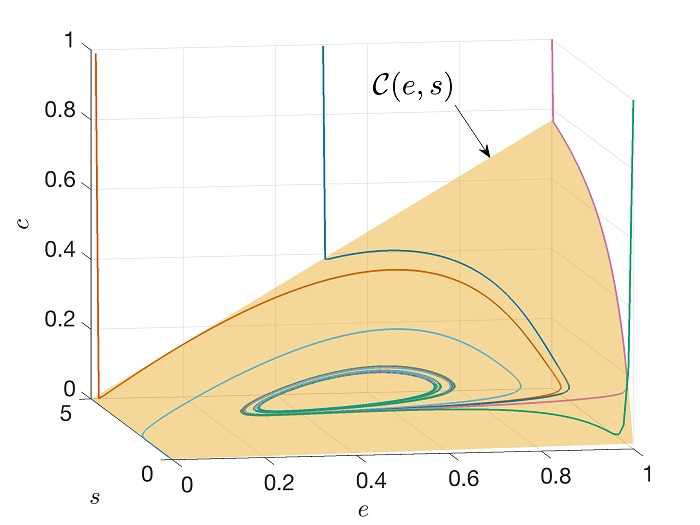
3.1. The ”Fast RNA” Case

Before analyzing system (21), we consider a special limit from which we will learn some valuable lessons: Suppose that the RNA dynamics is fast, i.e., that ${\epsilon }_2$ is vanishingly small. Then, using a standard result of singular perturbation theory for delay-differential equations [87,88], we can write the simplified system

$$\begin{array}{ll}{\epsilon }_1\dot{s}& =\kappa -s(e-c)+\alpha c,\end{array}$$

(22a)

$$\begin{array}{ll}\beta {\epsilon }_1\dot{c}& =s(e-c)-(\gamma +\beta {\epsilon }_1)c,\end{array}$$

(22b)

$$\begin{array}{ll}\dot{e}& =\rho \left(s(\theta -\delta )\right)-e.\end{array}$$

(22c)

This system is almost identical to one studied previously [39], except that the older model assumed that only the free enzyme decayed. This allowed the enzyme-substrate complex (C) to act as a protected reservoir of the enzyme, so that there was no upper limit on the allowed values of $k_{\mathrm{in}}$. This is not the case for the family of models studied in this contribution, which are subject to the constraint (12).

Like the previously studied model [39], the system (22) displays an Andronov–Hopf bifurcation. Thus, it should have a two-dimensional (slow/center/unstable) inertial manifold in the vicinity of this bifurcation. Let us suppose, for the sake of argument, that $\beta {\epsilon }_1\ll min({\epsilon }_1,1)$. Then we would expect to have an inertial manifold parameterizable in the form $c=\mathcal{C}(e,s)$. Our objective is to obtain an ODE model for the motion on the inertial manifold. Thus, we must eliminate Equation (22c) which contains the delayed term. Suppose that we have obtained the equation of the manifold, $c=\mathcal{C}(e,s)$. We can then obtain an ODE system representing the motion on this manifold by using Equation (22a,b), and solving the equation $c=\mathcal{C}(e,s)$ for e to close the system.

Our first task then is to obtain an approximation for the equation of the inertial manifold. We start, as usual, from the invariance equation

$$\dot{c}=\frac{\partial \mathcal{C}}{\partial e}\dot{e}+\frac{\partial \mathcal{C}}{\partial s}\dot{s}.$$

(23)

In this system, $\dot{e}$ depends on delayed values of s. This is a problem because Equation (23) is, in principle, a PDE for a manifold in the state space. Consider however expanding the nonlinearity in small powers of the delay:

$$\rho \left(s(\theta -\delta )\right)\approx \rho \left(s\right)-\delta {\left[\frac{d\rho }{ds}\dot{s}\right]}_{\delta =0}+\frac{{\delta }^2}{2}{\left[\frac{d^2\rho }{d{s}^2}{\dot{s}}^2+\frac{d\rho }{ds}\ddot{s}\right]}_{\delta =0}-\frac{{\delta }^3}{6}{\left[\frac{d^3\rho }{d{s}^3}{\dot{s}}^3+3\frac{d^2\rho }{d{s}^2}\dot{s}\ddot{s}+\frac{d\rho }{ds}\stackrel{⃛}{s}\right]}_{\delta =0}+\dots$$

(24)

As previously mentioned, we cannot substitute this expansion beyond the $O\left(\delta \right)$ term into Equation (22c) and numerically integrate the equations, as shown by El’sgol’ts [36] (pp. 284–285). For this reason, previous studies had truncated the small-delay expansion after the $O\left(\delta \right)$ term [32,49]. However, we can use this expansion to approximate the vector field implied by the delay equations [38], and in particular to compute inertial manifolds of the DDEs [33,40].

The quantities $\ddot{s}$ and $\stackrel{⃛}{s}$ (both evaluated at $\delta =0$) appearing in Equation (24) can be obtained by repeated differentiation of Equation (22a). For this particular model, we get

$${\left.\ddot{s}\right|}_{\delta =0}={\epsilon }_1^{-1}\left\{(c-e)\dot{s}-s\left[\rho \left(s\right)-e\right]+(s+\alpha )\dot{c}\right\}$$

(25)

and

$$\begin{array}{l}{\left.\stackrel{⃛}{s}\right|}_{\delta =0}={\left(\beta {\epsilon }_1^2\right)}^{-1}\{2\beta {\epsilon }_1\dot{s}\left[\dot{c}-\rho \left(s\right)+e\right]+\left[\beta (e-c)+s+\alpha \right]\left[\dot{s}(e-c)+s(\rho \left(s\right)-e)\right]\\ -\beta {\epsilon }_{1}s\left(\frac{d\rho }{ds}\dot{s}-\rho \left(s\right)+e\right)+\dot{c}\left[\beta (c-e)(s+\alpha )-(s+\gamma +\beta {\epsilon }_1)(\alpha +s)\right]\}.\end{array}$$

(26)

The approximate manifolds ${\mathcal{C}}_k^{\left(m\right)}$ will now have two indices: k to label the iterate, and m to indicate the last power of $\delta$ included in the expansion (24). The expansion contains powers of c, so in general it is not convenient (if it is even possible) to write down explicitly the functional equation. However, for $m=1$, we have, after labeling for iteration,

$${\mathcal{C}}_{k+1}^{\left(1\right)}=\frac{{\displaystyle es-\beta {\epsilon }_1(\rho \left(s\right)-e)\frac{\partial {\mathcal{C}}_k^{\left(1\right)}}{\partial e}+\beta (\kappa -es)\left(\delta \frac{\partial {\mathcal{C}}_k^{\left(1\right)}}{\partial e}\frac{d\rho }{ds}-\frac{\partial {\mathcal{C}}_k^{\left(1\right)}}{\partial s}\right)}}{{\displaystyle s+\gamma +\beta {\epsilon }_1-\beta (s+\alpha )\left(\delta \frac{\partial {\mathcal{C}}_k^{\left(1\right)}}{\partial e}\frac{d\rho }{ds}-\frac{\partial {\mathcal{C}}_k^{\left(1\right)}}{\partial s}\right)}}.$$

(27)

The $m=0$ case is recovered by setting $\delta =0$ in this equation. If we start iteration from the initial function ${\mathcal{C}}_0^{\left(1\right)}=0$, we get the following as the first iterate:

$${\mathcal{C}}_1^{\left(1\right)}=\frac{es}{s+\gamma +\beta {\epsilon }_1}.$$

(28)

A zero initial function is often a good choice for initializing this style of iteration. In the case of ordinary chemical models, this naïve initial function generally returns the steady-state approximation as the first iterate [1,5,80], which is a useful property of this class of iterative schemes.

Note that Equation (28) is readily invertible with respect to e except when $s=0$. There is therefore some hope that more accurate expressions for the inertial manifold generated by iteration will also be locally invertible, and therefore that the model reduction scheme described above will work.

Equation (27) can be iterated analytically using a symbolic algebra language. The $m=2$ functional equation gives a quadratic equation in c. It could also be iterated analytically, but numerical iteration was used for $m=2$ and $m=3$ instead. Iteration of Equation (27) and of its implicit counterparts for $m>1$ converges very quickly. The differences between the manifolds obtained for different values of m are essentially negligible (Figure 4).

We can draw a few lessons from these calculations:

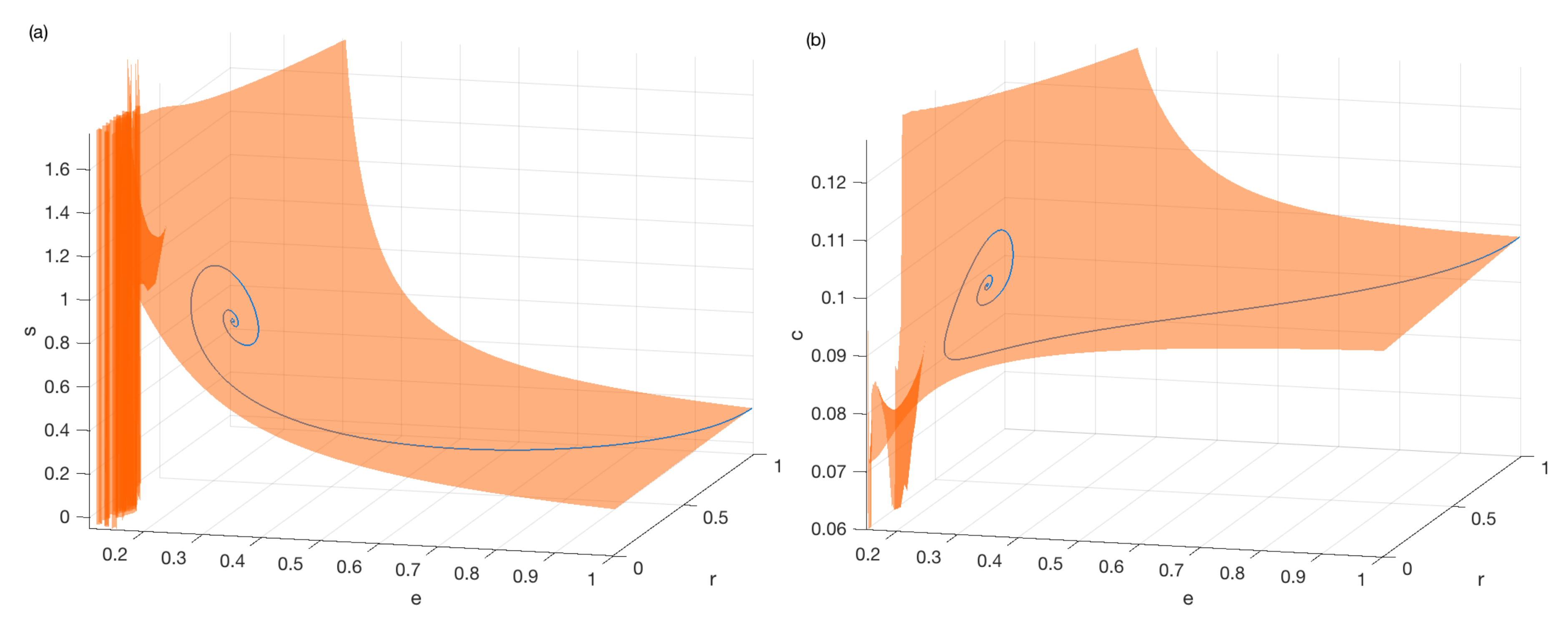
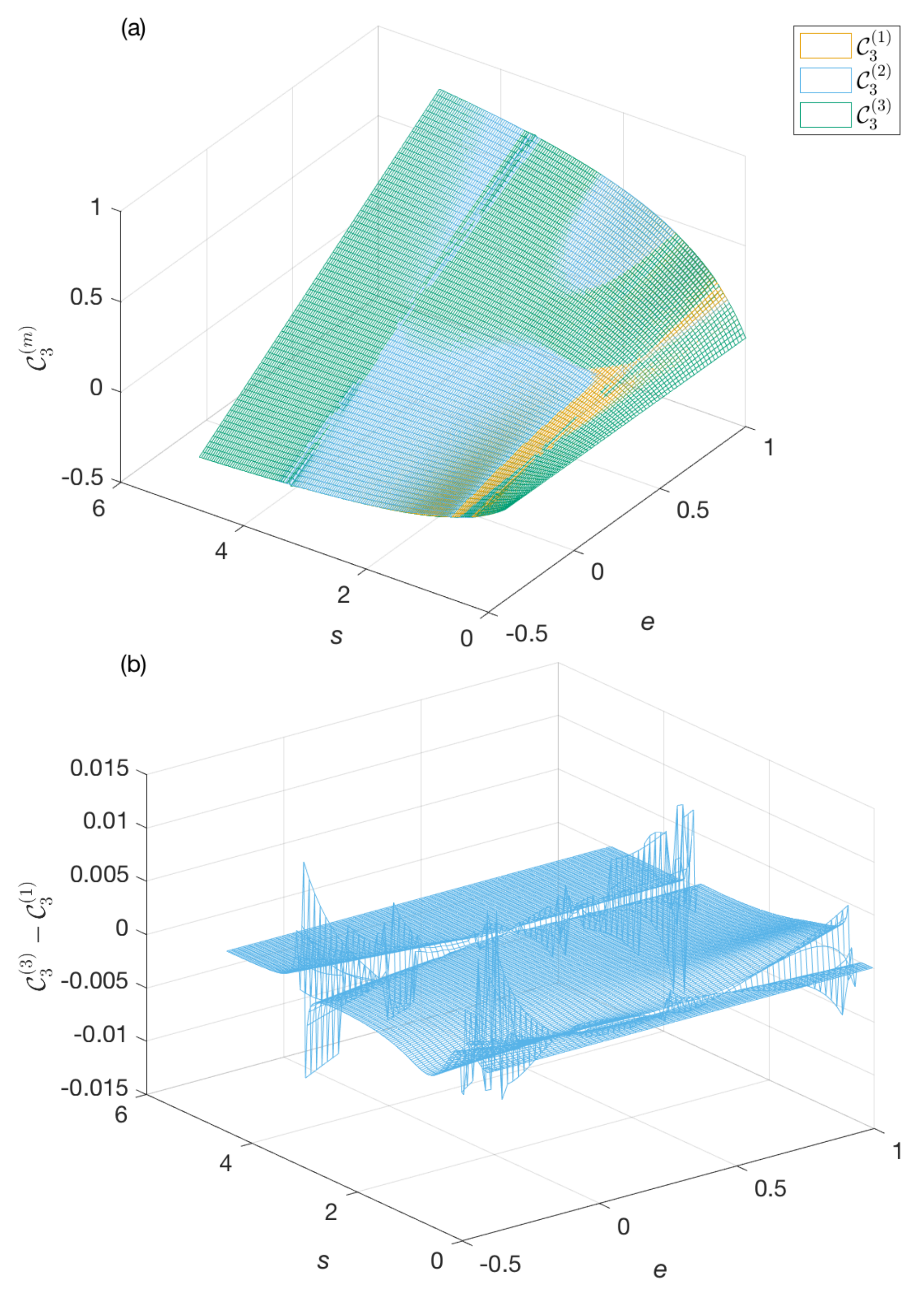
• Because the manifolds computed for different values of m are essentially identical, it appears that the higher-order corrections to the vector field are unnecessary to capture the dynamics, at least in the parameter regime of Figure 4.
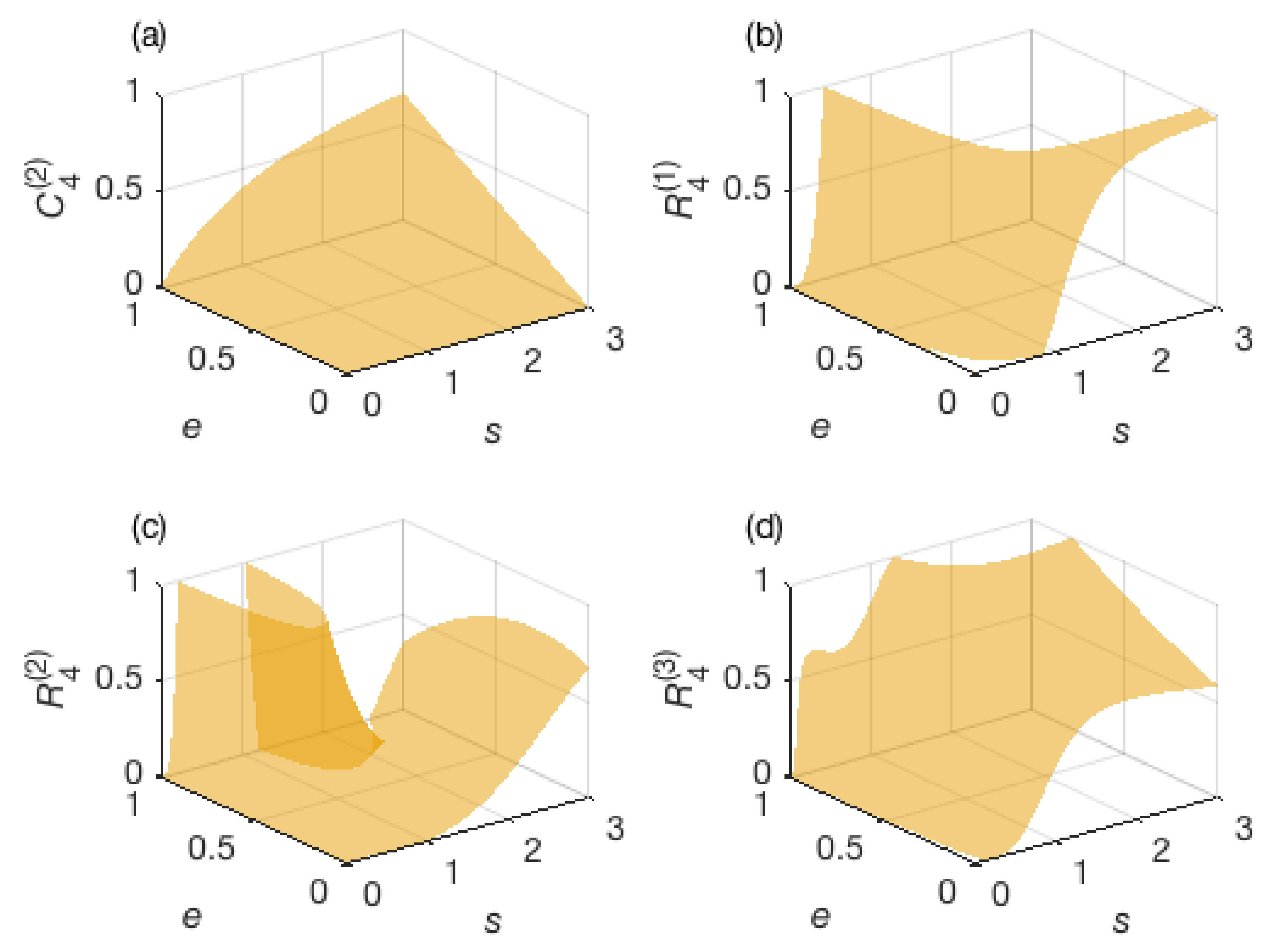
• The calculation for $m=1$ (even if carried out numerically) is much better behaved than for larger values of m. In the numerical calculations with larger m, localized imperfections appear in the manifolds. A simple routine was developed for removing these imperfections, essentially by interpolating through the region where they appear, but we can see from Figure 4b that there are small residual artifacts in the surfaces. (${\mathcal{C}}_3^{\left(1\right)}$, on the other hand, is perfectly smooth.)
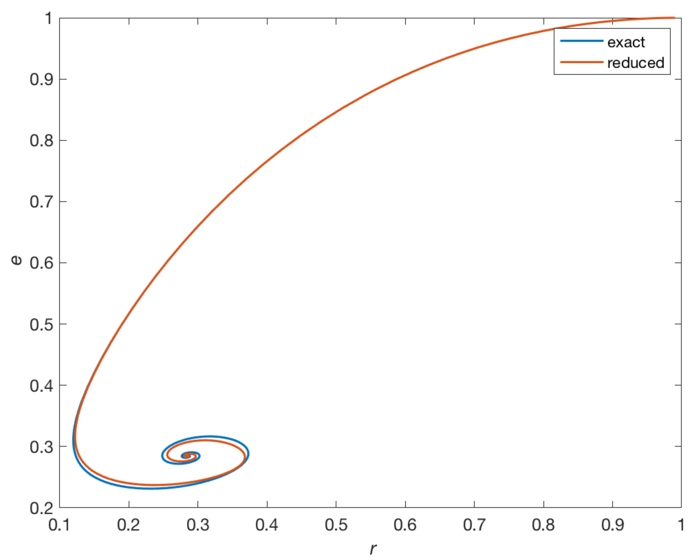
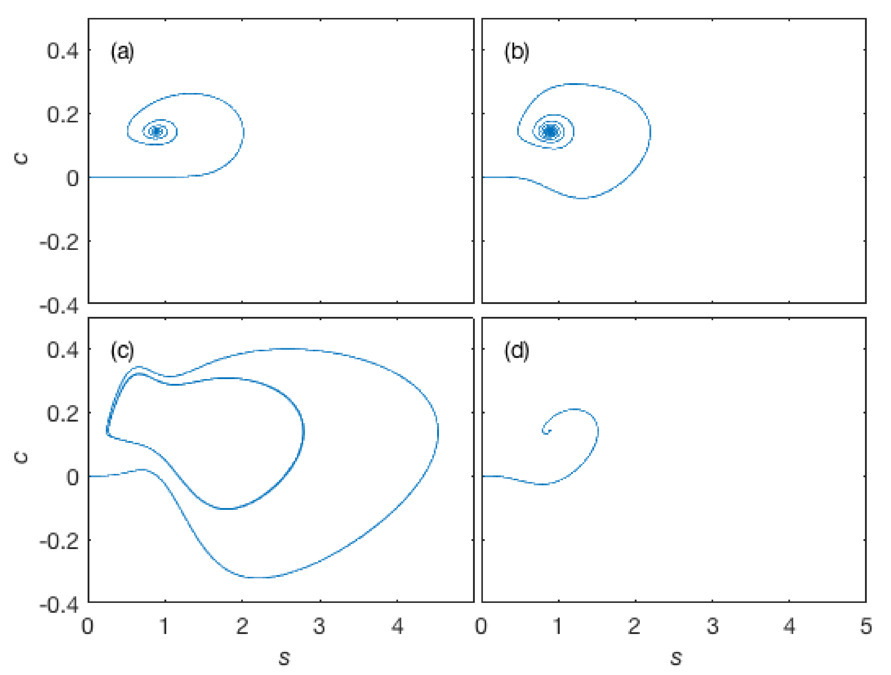
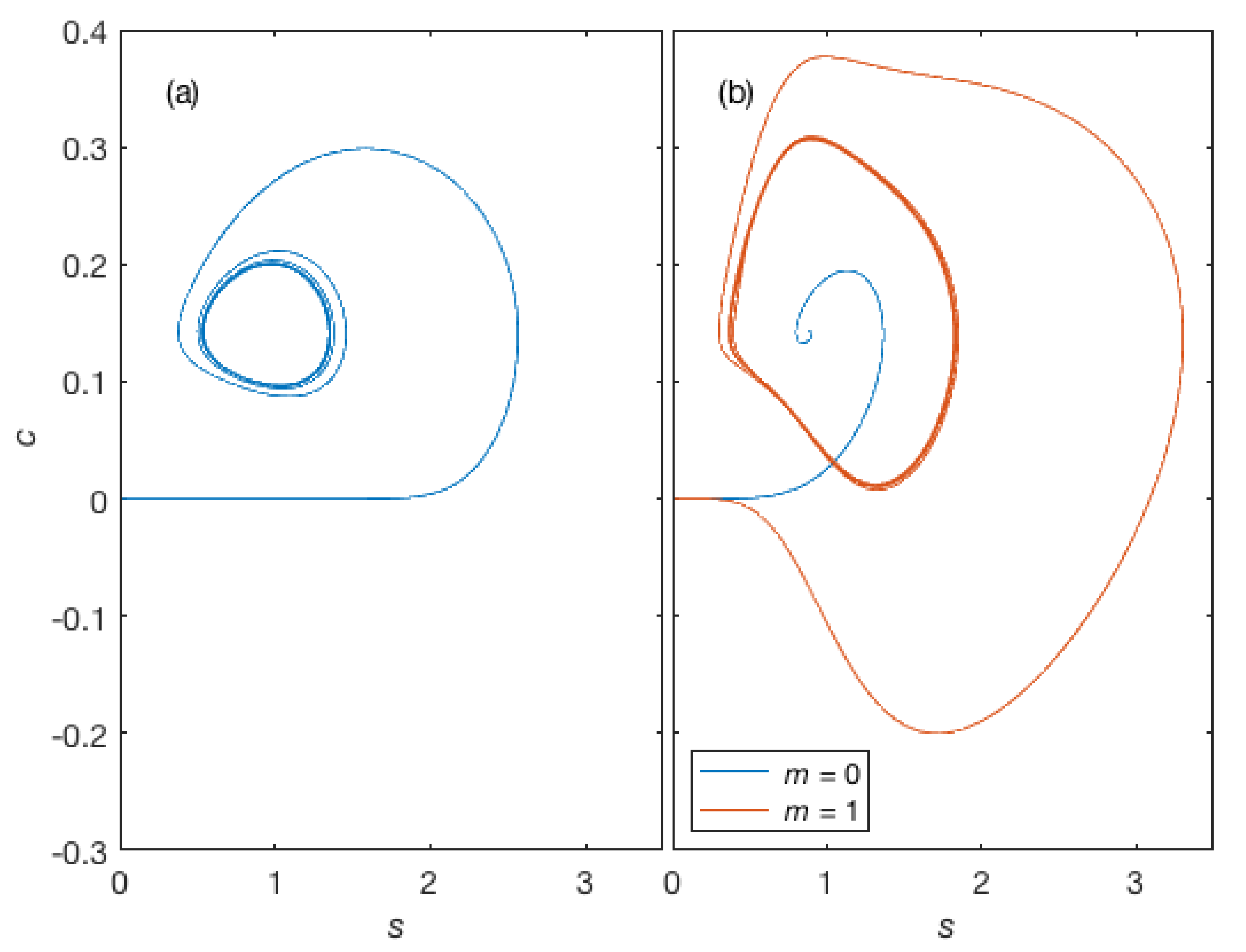
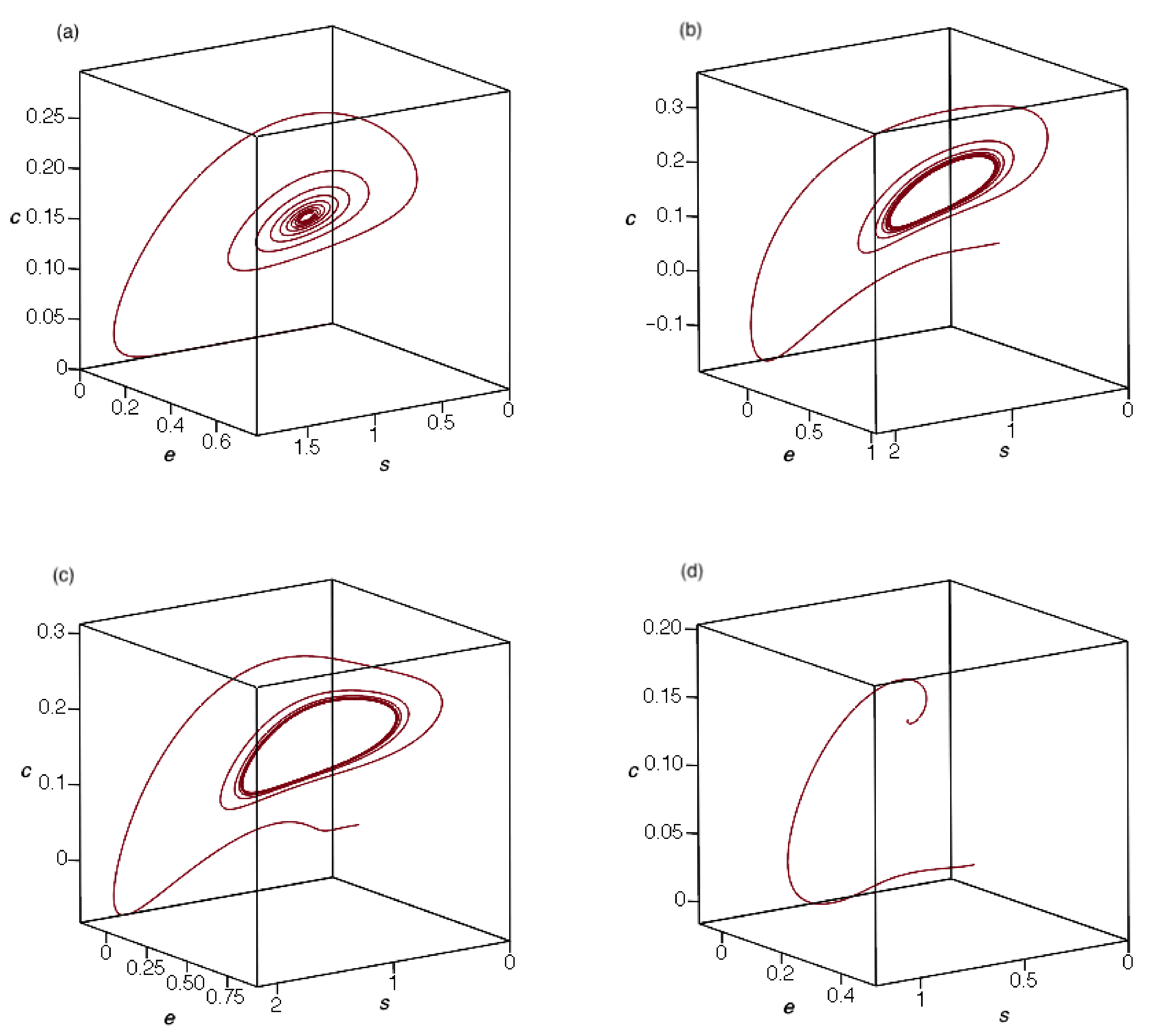
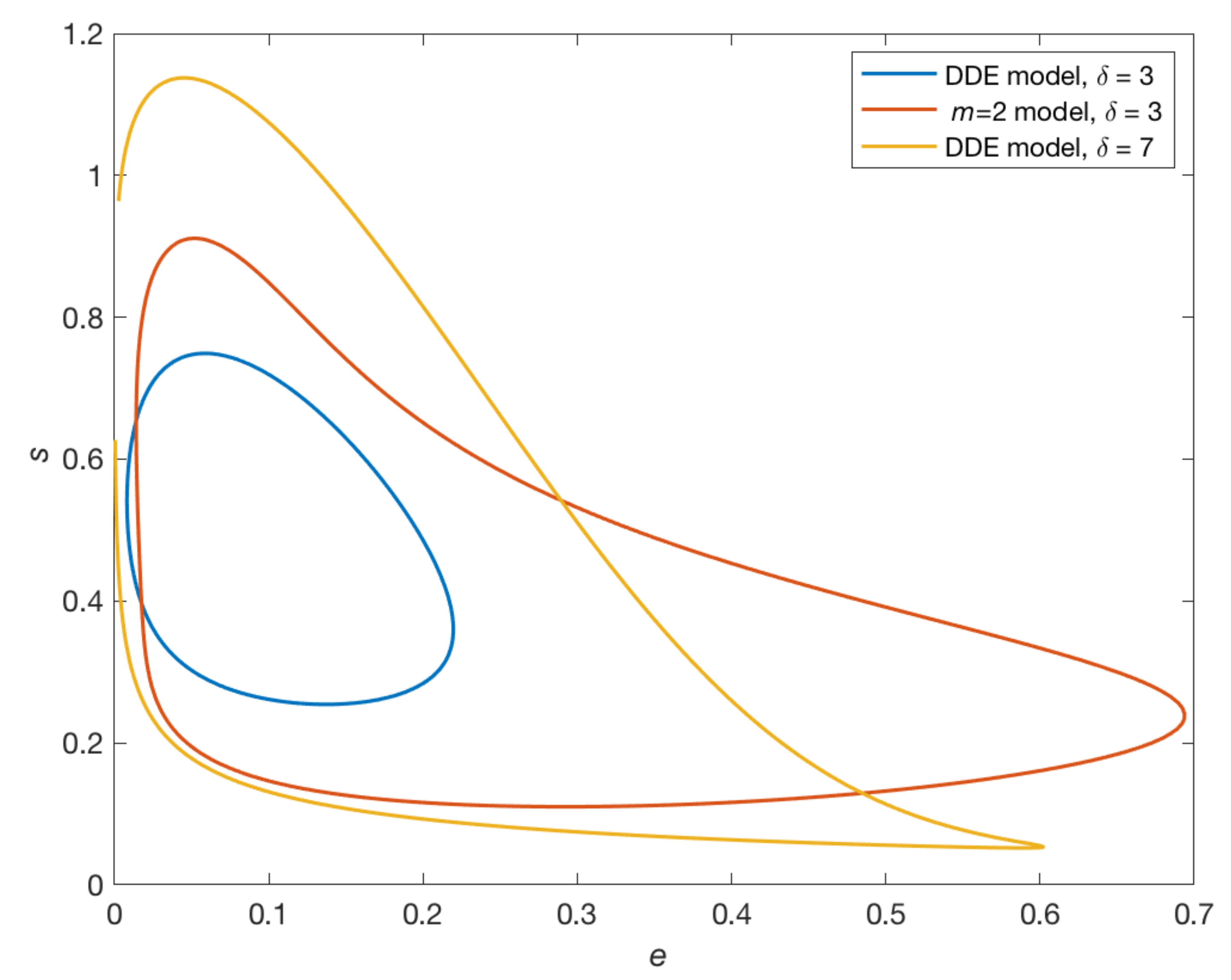
• If we integrate the model reduced to the inertial manifold, the $m=1$ reduced model best reproduces the trajectories of the three-variable DDE model (Figure 5). After an unphysical excursion to negative concentrations, the $m=1$ model reproduces the trajectory of the three-variable model reasonably well. On the other hand, the $m=2$ model has a limit cycle, which does not appear in the three-variable model until $\delta$ is above 0.54, and the $m=3$ model is excessively damped. The negative concentrations in the reduced model may be due to a poor representation of the inertial manifold near the $c=0$ axis, and would be an interesting subject for future investigations. The more serious misbehavior of the $m=2$ and $m=3$ models is likely due to a compounding of numerical issues, mostly the difficulties in solving the functional equations accurately in certain parts of the surface, numerical error during the inversion of the relation $c={\mathcal{C}}_k^{\left(m\right)}(e,s)$, and of course the interaction of these two factors.

Finally, note that the $\delta$ dependence of the inertial manifold is dynamically significant. The model without a delay (i.e., $m=0$) does not have an Andronov–Hopf bifurcation, but the $m=1$ ODE model does, as seen in Figure 6. The limit cycle in the $m=1$ model is a little larger than that in the DDE model, and is a little distorted. Nevertheless, there is clearly a wide range of parameters near the Andronov–Hopf bifurcation where the two models have similar behavior. In past work, it was found that an $m=1$ model accurately reproduced the Andronov–Hopf bifurcation curve of a related DDE model [39]. Although such a calculation has not been done for this model in order to focus on other issues, it seems clear that this will be true for this model as well.

3.2. Elimination of the Fastest Relaxation Mode

We now return to the original four-variable model including RNA, enzyme, substrate and enzyme–substrate complex, Equation (21). Let us suppose that we want to develop a state-space model, i.e., carry out a minimal reduction in which we eliminate the delay and obtain ODEs for the dynamics in a three-dimensional state space by computing a three-dimensional inertial manifold in the four-dimensional state space. As discussed previously, for “normal” parameters, i.e., parameter sets with ${\epsilon }_1\ll {\epsilon }_2\ll 1$, the system has three distinct time scales: fast enzyme kinetics, moderately fast mRNA dynamics, and slow dynamics of the total amount of enzyme. In this parameter range, the fastest variable, which is the one whose geometry will be most appropriate to this reduction, will be either s or c, depending on the values of $\beta$ and $\gamma$. (Either $\beta <1$ or $\gamma \gg \alpha$ would tend to make c the fastest variable.) However, the delay appears in the equation for r, so this is the variable in which we need to approximate the dynamics on the slow manifold in order to obtain the desired reduction. Let us say, for the sake of argument, that c is the fastest variable. We can compute an (approximate) inertial manifold in the form $c=\mathcal{C}(e,r,s)$ as we did in the previous section. We could then, in principle, have a reduced model that consists of the following set of differential-algebraic equations:

$$\begin{array}{ll}{\epsilon }_1\dot{s}& =\kappa -s(e-c)+\alpha c,\end{array}$$

(29a)

$$\begin{array}{ll}\beta {\epsilon }_1\dot{c}& =s(e-c)-(\gamma +\beta {\epsilon }_1)c,\end{array}$$

(29b)

$$\begin{array}{ll}\dot{e}& =r-e,\end{array}$$

(29c)

$$\begin{array}{ll}c& =\mathcal{C}(e,r,s).\end{array}$$

(29d)

As we did for the three-variable model, the last of these equations could in principle be numerically inverted to give us a value of r for any given c, e and s, thus closing the system. The problem is that c depends only indirectly on r through e. This has the result of making $\partial c/\partial r$ on the manifold small and difficult to compute accurately. The inversion process is therefore numerically ill-conditioned, so that a useful reduction is not obtained. Accordingly, in the usual parameter regime, a three-variable ODE model is not available.

The assumption that ${\epsilon }_2$ is larger than ${\epsilon }_1$ will be true for the vast majority of enzyme synthesis/catalysis systems, but is not necessarily so. Values of ${\epsilon }_2$ in a mouse cell line can be calculated directly from the data of Schwanhausser and coworkers [67], yielding values in the range of $1.5\times {10}^{-3}$ to 46, with a median of 0.20. The same data set gives a maximum value of $k_{dE}$ of $3.9\times {10}^{-4}{\mathrm{s}}^{-1}$. For prokaryotes, values larger than this by an order of magnitude are possible [89]. Rate constants for enzyme-substrate association ($k_1$) can be as low as ${10}^3{\mathrm{M}}^{-1}{s}^{-1}$ [90,91]. Since enzyme concentrations in excess of $1\mathsf{\mu }\mathrm{M}$ are routinely seen in vivo [92], values of ${\epsilon }_1>{\epsilon }_2$ are certainly within the realm of possibility. In the extreme, this parameter regime leads to the three-variable model. Since ${\epsilon }_2$ is never vanishingly small, it is worth reexamining this case using the manifold construction techniques we have been studying to compute an ODE state-space model valid when ${\epsilon }_2$ is small, but not vanishingly so. If ${\epsilon }_2$ is smaller than both ${\epsilon }_1$ and $\beta {\epsilon }_1$, then r is the fastest variable in the system, and we should be able to directly eliminate it by computing an inertial manifold of the form $r=\mathcal{R}(e,s,c)$. This ansatz leads to the invariance equation

$$\dot{r}=\frac{\partial \mathcal{R}}{\partial e}\dot{e}+\frac{\partial \mathcal{R}}{\partial s}\dot{s}+\frac{\partial \mathcal{R}}{\partial c}\dot{c}.$$

(30)

The general plan is as before: we will use the expansion (24) to replace the delayed term in Equation (21c) prior to substitution into the functional equation, and then iteratively solve the invariance equation for $\mathcal{R}(e,s,c)$ from some suitable initial guess. If we expand $\rho$ to first order in $\delta$, the resulting iteration is

$$\begin{array}{ll}{\mathcal{R}}_{k+1}^{\left(1\right)}=& \{\rho \left(s\right)+{\epsilon }_{2}e\frac{\partial {\mathcal{R}}_k^{\left(1\right)}}{\partial e}-\left[\kappa -s(e-c)+\alpha c\right]\left(\frac{\delta }{{\epsilon }_1}\frac{d\rho }{ds}+\frac{{\epsilon }_2}{{\epsilon }_1}\frac{\partial {\mathcal{R}}_k^{\left(1\right)}}{\partial s}\right)\\ & -\frac{{\epsilon }_2}{\beta {\epsilon }_1}\frac{\partial {\mathcal{R}}_k^{\left(1\right)}}{\partial c}\left[s(e-c)-(\gamma +\beta {\epsilon }_1)c\right]\}{\left(1+{\epsilon }_2\frac{\partial {\mathcal{R}}_k^{\left(1\right)}}{\partial e}\right)}^{-1}.\end{array}$$

(31)

To go beyond first order, we need

$$\ddot{s}=\frac{1}{{\epsilon }_1}\left[-\dot{s}(e-c)-s\dot{e}+\dot{c}(s+\alpha )\right]$$

(32)

and

$$\begin{array}{ll}\stackrel{⃛}{s}=& {\left(\beta {\epsilon }_1^2\right)}^{-1}\{-\beta (\dot{e}-\dot{c})(\kappa +\alpha c)-\beta (e-c)\left[\alpha \dot{c}-\dot{s}(e-c)\right]+2\beta s(\dot{e}-\dot{c})(e-c)\\ & -\beta {\epsilon }_1\left[\dot{s}(r-e)+\frac{s}{{\epsilon }_2}(\rho \left(s\right)-r)-s\dot{e}\right]+\dot{s}\left[s(e-c)-(\gamma +\beta {\epsilon }_1)c\right]\\ & +(s+\alpha )\left[\dot{s}(e-c)+s(\dot{e}-\dot{c})-(\gamma +\beta {\epsilon }_1)c\right]\}.\end{array}$$

(33)

Up to third order in $\delta$, it is possible to analytically isolate $\mathcal{R}$ from Equation (30). The functional equations for ${\mathcal{R}}^{\left(m\right)}$ become more and more complicated, but the work is easily carried out in a symbolic algebra system. Iteration of these functional equations can thus be carried out analytically, also in a symbolic algebra system. The size of the algebraic expressions generated by the iteration process grows rapidly, limiting the number of iterates that can practically be computed. Maple, the symbolic algebra system used in this study, lacks a function that gives a useful measure of the size of an expression. A simple workaround is to have Maple generate (say) Matlab code, and to count the number of bytes in these files. The optimize option was not used in order to measure the size of the expressions as stored by Maple. Also note that it is not feasible to use simplify() on the expression generated during iteration as the computation time required to execute this function grows very rapidly with the size of the expression.

Table 1. Sizes of expressions generated during the iterative solution of Equation (30) for different iteration levels (k) and orders of expansion (m) with respect to $\delta$. Values are given in characters, with SI prefixes used to represent larger values.

k	$\mathit{m}=1$	2	3
1	152	628	4.07 k
2	4.15 k	26.9 k	190 k
3	252 k	2.09 M	14.3 M

shows the growth of the size of the expressions for the iterates with both k and m. Note particularly the enormous sizes of the expressions generated for $m=2$ and 3 after a modest number of iterations. This is another reason to prefer the lowest-m expansion that suffices to reproduce the behavior of the original system.

If we take as an initial guess ${\mathcal{R}}_0^{\left(1\right)}=0$, then from Equation (31) we get the following $O\left(\delta \right)$ first approximation to the inertial manifold:

$${\mathcal{R}}_1^{\left(1\right)}(e,s,c)=\rho \left(s\right)-\frac{\delta }{{\epsilon }_1}\left[\kappa -s(e-c)+\alpha c\right]\frac{d\rho }{ds}.$$

(34)

This is the simplest approximation to the inertial manifold that takes account of the delay. For $m=1$, there is no significant change in the shape of the manifold for $k>2$. This is difficult to show directly since we cannot plot a function of three variables. We could take cuts through this function at, say, different values of c, but these are not very enlightening. Instead, we compute trajectories of the reduced system using $r={\mathcal{R}}_k^{\left(m\right)}(e,s,c)$ for different values of k, and then calculate the scaled difference between iterates, the iteration error (IE):

$${\mathrm{IE}}_k^{\left(m\right)}\left(\theta \right)=\frac{2\left({\mathcal{R}}_k^{\left(m\right)}{\left(e\left(\theta \right),s\left(\theta \right),c\left(\theta \right)\right)}_k^{\left(m\right)}-{\mathcal{R}}_{k-1}^{\left(m\right)}{\left(e\left(\theta \right),s\left(\theta \right),c\left(\theta \right)\right)}_{k-1}^{\left(m\right)}\right)}{\left|{\mathcal{R}}_k^{\left(m\right)}{\left(e\left(\theta \right),s\left(\theta \right),c\left(\theta \right)\right)}_k^{\left(m\right)}\right|+\left|{\mathcal{R}}_{k-1}^{\left(m\right)}{\left(e\left(\theta \right),s\left(\theta \right),c\left(\theta \right)\right)}_{k-1}^{\left(m\right)}\right|}.$$

(35)

In this equation, ${\left(e\left(\theta \right),s\left(\theta \right),c\left(\theta \right)\right)}_k^{\left(m\right)}$ refers to a trajectory of the reduced model. This is a very stringent test because differences in frequency can cause large differences in the trajectories even if the overall dynamics are very similar. Figure 7 shows these iteration errors for a parameter set in the regime where we expect to be able to carry out this reduction. Near the initial condition, it is difficult to measure ${\mathrm{IE}}_k^{\left(m\right)}$ reliably because of the small denominator in Equation (35), so values of this statistic near $\theta =0$ should be ignored. For $k=2$, we see large-amplitude oscillations, indicating that the two manifolds are sufficiently different to cause a loss of coherence. When we calculate the next iterate, the iteration error becomes much smaller and loses any obvious periodicity, which is evidence of rapid convergence of the iterations. The same behavior is observed for higher values of m.

While iteration converges rapidly, it turns out that the reduced models are only qualitatively correct. Figure 8 shows trajectories of the DDE model as well as of the state-space ODE models. For the parameters chosen, the DDE model has a stable focus. On the other hand, the reduced models for $m=1$ and 2 have limit-cycle attractors, i.e., they undergo an Andronov–Hopf bifurcation at a smaller value of $\delta$ (keeping the other parameters constant) than the DDE model, near $\delta =0.84$ for the $m=1$ reduced model vs. $\delta =1.04$ for the DDE model. As for the $m=3$ reduced model, it is much more strongly damped than the DDE model, and it fails completely if we try to increase $\delta$ too much.

Note that the value of ${\epsilon }_2$ chosen for the calculations of Figure 7 and Figure 8 is not particularly small compared to ${\epsilon }_1$. The $m=1$ and $m=2$ state-space models are qualitatively correct, even if there are some quantitative discrepancies such as the exact parameter values at the Andronov–Hopf bifurcation. The agreement improves if we decrease ${\epsilon }_2$.

3.3. Computing a Two-Dimensional Inertial Manifold

Given the Andronov–Hopf bifurcation in this system, the lowest-dimensional description of the dynamics that captures the behavior to either side of the bifurcation is motion on a two-dimensional inertial manifold. As argued previously, the most likely parameter regime is one in which c and s are the fast variables. However, as in the three-variable model, this leads to an implicit manifold representation problem which will be left for future study. Rather, we consider the regime where $\beta \ll 1$ and ${\epsilon }_2\ll \{{\epsilon }_1,1\}$. This is the easiest biochemically plausible case since r is then one of the fast variables, which means that the delay can be directly eliminated. The other fast variable in this case is of course c. These considerations imply a parameterization of the manifold $c=\mathcal{C}(e,s)$, $r=\mathcal{R}(e,s)$. The corresponding invariance equations are

$$\begin{array}{ll}\dot{c}& =\frac{\partial \mathcal{C}}{\partial e}\dot{e}+\frac{\partial \mathcal{C}}{\partial s}\dot{s},\end{array}$$

(36a)

$$\begin{array}{ll}\dot{r}& =\frac{\partial \mathcal{R}}{\partial e}\dot{e}+\frac{\partial \mathcal{R}}{\partial s}\dot{s}.\end{array}$$

(36b)

The delayed term does not appear in Equation (36a), so the functional iteration for $\mathcal{C}(e,s)$ is the same regardless of the delay expansion order:

$${\mathcal{C}}_{k+1}^{\left(m\right)}=\frac{{\displaystyle es-\beta {\epsilon }_1\frac{\partial {\mathcal{C}}_k^{\left(m\right)}}{\partial e}\left({\mathcal{R}}_k^{\left(m\right)}-e\right)-\beta \frac{\partial {\mathcal{C}}_k^{\left(m\right)}}{\partial s}(\kappa -es)}}{{\displaystyle s+\gamma +\beta {\epsilon }_1+\beta \frac{\partial {\mathcal{C}}_k^{\left(m\right)}}{\partial s}(s+\alpha )}}.$$

(37)

(${\mathcal{C}}_k^{\left(m\right)}$ will eventually depend on m because of its dependence on ${\mathcal{R}}_k^{\left(m\right)}$.) The functional equations for $\mathcal{R}(e,s)$ can also be derived analytically, although for $m>1$, the derivation is best left to a symbolic algebra system. For $m=1$, we have

$${\mathcal{R}}_{k+1}^{\left(1\right)}=\frac{{\displaystyle \rho \left(s\right)-\left(\frac{\delta }{{\epsilon }_1}\frac{d\rho }{ds}+\frac{{\epsilon }_2}{{\epsilon }_1}\frac{\partial {\mathcal{R}}_k^{\left(1\right)}}{\partial s}\right)\left[\kappa -es+{\mathcal{C}}_{k+1}^{\left(1\right)}(s+\alpha )\right]+{\epsilon }_{2}e\frac{\partial {\mathcal{R}}_k^{\left(1\right)}}{\partial e}}}{{\displaystyle 1+{\epsilon }_2\frac{\partial {\mathcal{R}}_k^{\left(1\right)}}{\partial e}}},$$

(38)

assuming chained iteration, $\mathcal{C}$ first. Even starting with our usual naïve initial function of ${\mathcal{R}}_0^{\left(m\right)}=0$, we see that ${\mathcal{R}}_1^{\left(1\right)}$ will depend on $\delta$. Corrections to the slow manifold due to the delay therefore enter at a level equivalent to the application of the steady-state approximation.

From the functional Equations (37) and (38), we can see that at this level of approximation of the vector field, corrections to the manifold due to the delay depend on $\delta /{\epsilon }_1$. Thus, the delay will become less significant to the slow dynamics at small values of $\delta$ or large values of ${\epsilon }_1$. Here we see an example where the analysis tells us something that might have been difficult to intuit: In terms of the original dimensional parameters, the condition $\delta /{\epsilon }_1\ll 1$ becomes $k_1{E}_{\max }\ll {\tau }^{-1}$. Thus, if the association of the enzyme and substrate is sufficiently slow compared to the gene expression cycle, the delay associated with this cycle should have a negligible effect on the geometry of the slow manifold and, at least from the perspective of the motion on the two-dimensional slow manifold, an ODE model neglecting the transcription and translation delays would be appropriate. Note that this says nothing about the transients, which could still be very different between the models with and without delays.

The reduced model obtained from Equation (21) for a computed manifold $\left(\mathcal{C}\right(e,s),\mathcal{R}(e,s\left)\right)$ is the planar system

$$\begin{array}{ll}{\epsilon }_1\dot{s}& =\kappa -es+\mathcal{C}(e,s)\left(s+\alpha \right),\end{array}$$

(39a)

$$\begin{array}{ll}\dot{e}& =\mathcal{R}(e,s)-e.\end{array}$$

(39b)

Given explicit functional equations, we could try to carry out the iterations analytically in a symbolic algebra system, but again the expressions quickly grow to the point where they cannot practically be handled, so numerical iteration was used. The second iterate was obtained analytically for each m and used to verify reasonable accuracy of the numerical scheme. These differences (not shown) are generally very small ($O\left({10}^{-6}\right)$ or less), except at the $s=0$ edge. Note that the boundary of the computational domain is often a source of instability in this class of iterative methods [50,86]. Now consider the first iterate of Equation (38) starting from the naïve initial function:

$${\mathcal{R}}_1^{\left(1\right)}=\rho \left(s\right)-\frac{\delta }{{\epsilon }_1}\frac{d\rho }{ds}\left[\kappa -es+{\mathcal{C}}_1^{\left(1\right)}(s+\alpha )\right].$$

(40)

For $n>1$, $d\rho /ds\to 0$ as $s\to 0$. Thus, ${\mathcal{R}}_1^{\left(1\right)}$ itself tends to zero as $s\to 0$. Estimating the derivative in this region therefore involves taking differences of small quantities, which is difficult to do accurately, resulting in larger errors in the numerical iteration process in this region. Fortunately, these errors do not destabilize the iterative scheme, at least if we stop iteration as soon as reasonable convergence is achieved. Convergence is (again) very fast, so three or four iterates are sufficient to reduce the iteration error below the threshold where it has any observable effect on the dynamics. Because the approximated manifolds are now paired surfaces $\mathcal{C}(e,s)$ and $\mathcal{R}(e,s)$, they are readily visualized.

Figure 9 shows the computed inertial manifolds at various levels of truncation, m. Despite its coupling to $\mathcal{R}$ (Equation (37)), $\mathcal{C}$ depends very little on m, so a representative approximation is shown. On the other hand, the shapes of the ${\mathcal{R}}^{\left(m\right)}$ surfaces are dramatically different. This is a possible sign of a divergent series in $\delta$. (Note that $\delta$ is not particularly small here.) However, which representation of the inertial manifold is the best?

A simple way to answer the latter question is to look at trajectories. For the parameters of Figure 9, the DDE model has a limit cycle (Figure 10). The system reduced to the $m=1$ approximate inertial manifold also has a limit cycle (not shown), but this limit cycle wanders out of the positive quadrant of the $(e,s)$ plane. We might accept unphysical excursions of trajectories started from some initial conditions, but an unphysical attractor is not acceptable in any potential application. The $m=2$ attractor is, on the other hand, an entirely sensible-looking limit-cycle entirely contained in the positive quadrant, although it is too large and of a different shape than the limit cycle of the DDE model (Figure 10). The significantly larger size of the limit cycle in the $m=2$ reduced model is associated with an Andronov–Hopf bifurcation that occurs at a smaller value of $\delta$ than in the DDE model. For $m=3$, all we get is a strongly damped oscillation (not shown). It thus seems that the $m=2$ approximation is the best representation of the inertial manifold available in the context of this method for these parameters.

The observation that the Andronov–Hopf bifurcation is advanced in the $m=2$ reduced model relative to the original DDE model raises an interesting question, particularly since the limit cycle in the reduced model has a different shape than that in the DDE model: are the dynamics of the reduced model simply shifted along the $\delta$ axis in the parameter space? Along with the two limit cycles already discussed, Figure 10 shows the attractor of the DDE model at a larger value of $\delta$. This limit cycle has a shape much more like that of the reduced model. Remarkably then, the small-delay approximation captures the rough shape of the vector field on the inertial manifold, but at a somewhat different value of $\delta$ than the one used in constructing the manifold. This suggests that there may exist a transformation of the $\delta$ axis that would bring the two models into closer correspondence. It is not clear whether a systematic method could be developed to estimate the mapping from the true value of $\delta$ to the effective $\delta$ of the reduced model. This would be an interesting avenue for future investigation.

Finally, note that the graph of $\mathcal{R}(e,s)$ for the best representation of the slow manifold, ${\mathcal{R}}^{\left(2\right)}$ (Figure 9c) has a complex shape that could not be predicted from intuition alone. The question of whether this surface could be systematically explored in realistic experiments is also left for future investigation.

4. Discussion

Throughout the examples considered in this paper, we consistently obtained rapid convergence of the iterative schemes at fixed m. On the other hand, the expansion of the delayed nonlinearity in powers of $\delta$ was more delicate. Sometimes, the best results were obtained for $m=1$, and sometimes for $m=2$. It seems likely, given the results of Chicone [33,38,40] that there is no fundamental limitation on the order of expansion in the delay, and that the “best” order of expansion therefore depends on the model and parameters. In Chicone’s work, it was assumed that the delay was sufficiently small for the Taylor series to converge. Here, relatively large values of the delays have been considered, and convergence is not assured, but useful results can still be obtained provided we pick the “correct” order of expansion. The situation appears to be (at least) analogous to asymptotic series, where we get sensible approximations provided we cut off the expansion as soon as it starts to diverge [93]. Now that the method has been shown to give reasonable results in a number of challenging cases, the stage is set for a more deliberate analysis of its mathematical properties.

Despite the relatively large values of the delay used in this study, it was possible to calculate manifolds on which the dynamics are at least qualitatively correct. Note that the calculations were carried out to either side of the Andronov–Hopf bifurcation, even though results were not reported for every case tried. Thus, the method proposed here is able to represent inertial manifolds of DDEs over a range of parameters. This raises the question of whether there is some other development of the delay term that could be used. The Galerkin approximation method of Chekroun and coworkers [34] has already been mentioned. As a general point, it would be useful to have a variety of approximate transformations of delay equations valid in different parameter regimes.

Scaling played an important role throughout the work reported here. For every model variation analyzed, values of the singular perturbation parameters ${\epsilon }_1$, ${\epsilon }_2$ and $\beta$ would inform our choice of representations of the manifold. When the correct representation was chosen, rapid convergence of the iterative process was always obtained. In some calculations not reported here, choosing the “wrong” representation for the parameter range considered always led to difficulties with the iterative method, essentially because the manifolds were nearly vertical in parts of the state space. When analyzing smaller models for which scaling is practical, especially if we have some idea of the relevant parameter values, it is therefore well worth investing some time into a scaling analysis. This is, of course, not an original recommendation [63,65].

Implicitly, in selecting the representations of the manifolds in the delay model, we assumed that a version of Fenichel’s geometric singular perturbation theory [12] and, in particular, of his persistence and smoothness results [11], extended to inertial manifolds. Others have made the same assumption [94]. Chicone has shown that similar persistence and smoothness results hold using the delay as the small parameter in the singular perturbation expansion [33]. In Chicone’s approach, the singular limit is an ODE. The singular limit of systems such as (21) can be a set of DDEs with an algebraic constraint, or a set of ODEs with an algebraic functional constraint (e.g., $\rho \left(s\right(\theta -\delta \left)\right)=r\left(\theta \right)$ if ${\epsilon }_2\to 0$). To the author’s knowledge, persistence and smoothness of inertial manifolds for such systems has not been systematically studied. This is clearly an important area for future work. Given Chicone’s work and other extensions of singular perturbation theory to DDEs [87,88], it seems likely that such an extension of Fenichel’s results could be obtained.

Given the self-correcting nature of the iteration process, it is not necessary for the numerical iterates to be extremely accurate, provided they are smooth. Calculation of the derivatives is the main source of purely numerical instabilities. (There is also the possibility that the iteration scheme itself is unstable [48,49].) As noted earlier, the derivatives are currently computed by finite differences, with extrapolation used at the edges to avoid well-known difficulties with this class of iterative methods due to poor derivative estimates at the boundary of the computational domain [50,86]. Making the mesh tighter will make the derivative estimates more accurate in highly curved regions at the cost of potentially losing significant figures. However, the results are not highly sensitive to the computational mesh, provided we avoid making it too tight. What does matter is making sure to extend the mesh far enough to catch the full trajectory, even if this trajectory will wander into the unphysical, negative region of state space, as frequently happens to trajectories started near the boundary in these models (Figure 5, Figure 6 and Figure 8). Since this was not expected at first, the computational domain was generally set up to only include the part of the positive orthant likely to be visited. When trajectories wandered out of this region, the simulations had to be stopped, and the manifold recomputed in an extended region of state space that would hopefully be sufficient to accommodate the entire trajectory. The combustion community has often faced a similar problem, i.e., a lack of a priori knowledge of the region of the very high-dimensional phase space to be visited in a simulation. Their solution has been to extend the representation of the manifold as needed in directions visited by trajectories [95]. When the inertial manifold of a DDE needs to be computed numerically, a similar method could be used, first building a representation of the manifold in a region of the state space that we expect to be visited, and dynamically growing the manifold as needed.

When the iterative process resulting from the combined perturbative-iterative method proposed here can be carried out analytically, we end up with a small ODE model that may be amenable to computer-aided analysis. For example, the Andronov–Hopf bifurcation in the reduced model (39) will occur when

$$1-\frac{\partial \mathcal{R}}{\partial e}+\frac{1}{{\epsilon }_1}\left[e-\mathcal{C}-\frac{\partial \mathcal{C}}{\partial s}(s+\alpha )\right]=0,$$

(41)

with the left-hand side evaluated at the steady state, provided the quadratic discriminant of the characteristic polynomial (for which there is also a simple expression) is negative. Given analytic expressions for $\mathcal{C}(e,s)$ and $\mathcal{R}(e,s)$ and their dependence on the parameters, the Andronov–Hopf bifurcation condition is an explicit condition. Since steady-state coordinates depend on the parameters, to calculate Andronov–Hopf bifurcation curves, we solve the steady-state problem associated with Equation (39) along with (41) as a system of three equations in three unknowns, namely e, s and one free parameter at fixed values of the other parameters. This is an entirely straightforward numerical process [39]. By contrast, the Andronov–Hopf bifurcation problem for a DDE involves a characteristic quasipolynomial (involving both polynomial terms and terms in $e^{-\lambda \delta }$, where $\lambda$ is the characteristic value) [6] (Chapter 12). The real and imaginary parts of this characteristic quasipolynomial must be separated, and the real part set to zero. Obtaining an explicit bifurcation condition takes quite a bit of work. Of course, so does generating an inertial manifold. Which one is preferable becomes a matter of how often we will be solving the Andronov–Hopf bifurcation condition, as well as whether we have other uses for the representation of the manifold.

If we can only carry out the iteration numerically, it is in principle still possible to solve for Andronov–Hopf bifurcations using Equation (41), but it becomes much more laborious since the inertial manifold depends on the parameters. It will therefore be necessary to recompute the manifold (or at least a piece of it near the steady state) dynamically during the solution process. Instead of the iterative process used here, the method of invariant grids [96], which involves using a small number of points to represent a small part of the manifold, might be a more efficient way to represent and recompute the manifold in this case. An alternative might be to use continuation methods to compute the change in the manifold as parameters are changed [97]. It must be admitted though that working directly with the DDEs might be more efficient in these cases.

The model studied here was reducible to a single delay. However, gene expression models often involve multiple delays of different sizes [98,99,100,101] and will not in general be reducible to a single delay. The development of methods for calculating inertial manifolds would be particularly useful for such systems, since the complexity of linear stability analysis increases significantly with the number of delays. This is, to my knowledge, an entirely open problem area.

5. Conclusions

A method for computing inertial manifolds of systems of DDEs has been developed for models of the form

$$\begin{array}{ll}\dot{x}& =f\left(x\left(\theta \right),y\left(\theta \right)\right),\end{array}$$

(42a)

$$\begin{array}{ll}\dot{y}& =g\left(x\left(\theta \right),y\left(\theta \right),x_i(\theta -\delta )\right),\end{array}$$

(42b)

where x is an $(n-1)$-vector, y is a scalar, and $n>d$, the dimension of the manifold. Small parameters multiplying the derivatives, if they appear, can help guide the selection of manifold representations, but are not strictly necessary. This method involves a Taylor expansion of the delayed term in powers of the delay, followed by the use of an iterative method for the computation of the inertial manifold of the approximated vector field. In favorable cases, a computer algebra system can be used to obtain fully analytic approximations, with all of the attendant advantages. One notable property of the method developed here is that it can be applied to calculate inertial manifolds of any dimension. It is not limited to computing, for instance, two-dimensional center manifolds, as we saw in Section 3.2 where a three-dimensional manifold was obtained. At this time, the selection of the order of truncation of the Taylor series is based on ad hoc observations. Part of the difficulty in selecting the order of truncation is that the Taylor series is itself a complicated function of the state-space variables. (See, e.g., Equations (24)–(26)). Some cleverness will therefore be required to discover a systematic method for choosing the truncation order.

References

1. Roussel, M.R.; Fraser, S.J. On the Geometry of Transient Relaxation. J. Chem. Phys. 1991, 94, 7106–7113. [Google Scholar] [CrossRef]
2. Lam, S.H. Using CSP to Understand Complex Chemical Kinetics. Combust. Sci. Technol. 1993, 89, 375–404. [Google Scholar] [CrossRef]
3. Roussel, M.R.; Fraser, S.J. Invariant Manifold Methods for Metabolic Model Reduction. Chaos 2001, 11, 196–206. [Google Scholar] [CrossRef] [PubMed]
4. Lubich, C.; Nipp, K.; Stoffer, D. Runge-Kutta Solutions of Stiff Differential Equations Near Stationary Points. SIAM J. Numer. Anal. 1995, 32, 1296–1307. [Google Scholar] [CrossRef] [Green Version]
5. Fraser, S.J. The Steady State and Equilibrium Approximations: A Geometrical Picture. J. Chem. Phys. 1988, 88, 4732–4738. [Google Scholar] [CrossRef]
6. Roussel, M.R. Nonlinear Dynamics: A Hands-On Introductory Survey; IOP Concise Physics, Morgan & Claypool: San Rafael, CA, USA, 2019. [Google Scholar] [CrossRef]
7. Roberts, A.J. The Utility of an Invariant Manifold Description of the Evolution of a Dynamical System. SIAM J. Math. Anal. 1989, 20, 1447–1458. [Google Scholar] [CrossRef]
8. Hale, J.K.; Koçak, H. Dynamics and Bifurcations; Texts in Applied Mathematics; Springer: New York, NY, USA, 1991; Volume 3. [Google Scholar]
9. Carr, J. Applications of Centre Manifold Theory; Springer: New York, NY, USA, 1982. [Google Scholar]
10. Bogoliubov, N.N.; Mitropolsky, Y.A. The Method of Integral Manifolds in Nonlinear Mechanics. Contrib. Differ. Equ. 1963, 2, 123–196. [Google Scholar]
11. Fenichel, N. Persistence and Smoothness of Invariant Manifolds for Flows. Indiana U. Math. J. 1971, 21, 193–226. [Google Scholar] [CrossRef]
12. Fenichel, N. Geometric Singular Perturbation Theory for Ordinary Differential Equations. J. Differ. Equ. 1979, 31, 53–98. [Google Scholar] [CrossRef] [Green Version]
13. Bliss, R.D. Analysis of the Dynamic Behavior of the Tryptophan Operon of Escherichia coli: The Functional Significance of Feedback Inhibition. Ph.D. Thesis, University of California Riverside, Riverside, CA, USA, 1979. [Google Scholar]
14. Mahaffy, J.M. Cellular Control Models with Linked Positive and Negative Feedback and Delays. I. The Models. J. Theor. Biol. 1984, 106, 89–102. [Google Scholar] [CrossRef]
15. Lewis, J. Autoinhibition with Transcriptional Delay: A Simple Mechanism for the Zebrafish Somitogenesis Oscillator. Curr. Biol. 2003, 13, 1398–1408. [Google Scholar] [CrossRef] [Green Version]
16. Monk, N.A.M. Oscillatory Expression of Hes1, p53, and NF-κB Driven by Transcriptional Time Delays. Curr. Biol. 2003, 13, 1409–1413. [Google Scholar] [CrossRef] [Green Version]
17. Ahsen, M.E.; Özbay, H.; Niculescu, S.I. Analysis of Deterministic Cyclic Gene Regulatory Network Models with Delays; Birkhäuser: Cham, Switzerland, 2010. [Google Scholar] [CrossRef]
18. Mackey, M.C.; Santillán, M.; Tyran-Kamińska, M.; Zeron, E.S. Simple Mathematical Models of Gene Regulatory Dynamics; Springer: Cham, Switzerland, 2016. [Google Scholar]
19. Hale, J.K.; Lunel, S.M.V. Introduction to Functional Differential Equations; Springer: New York, NY, USA, 1993. [Google Scholar]
20. Hale, J.K. Dynamics and Delays. In Delay Differential Equations and Dynamical Systems; Busenberg, S., Martelli, M., Eds.; Springer: Berlin, Germany, 1990; pp. 16–30. [Google Scholar]
21. Luskin, M.; Sell, G.R. Approximation Theories for Inertial Manifolds. Math. Model. Numer. Anal. 1989, 23, 445–461. [Google Scholar] [CrossRef]
22. Fernández, A. The Steady-state Approximation as a Centre Manifold Elimination in Chemical Kinetics. J. Chem. Soc. Faraday Trans. 1986, 82, 849–855. [Google Scholar] [CrossRef]
23. Fabes, E.; Luskin, M.; Sell, G.R. Construction of Inertial Manifolds by Elliptic Regularization. J. Differ. Equ. 1991, 89, 355–387. [Google Scholar] [CrossRef] [Green Version]
24. Bélair, J.; Campbell, S.A. Similarity and Bifurcations of Equilibria in a Multiple-Delayed Differential Equation. SIAM J. Appl. Math. 1994, 54, 1402–1424. [Google Scholar] [CrossRef]
25. Wischert, W.; Wunderlin, A.; Pelster, A.; Olivier, M.; Groslambert, J. Delay-Induced Instabilities in Nonlinear Feedback Systems. Phys. Rev. E 1994, 49, 203–219. [Google Scholar] [CrossRef]
26. Qesmi, R.; Ait Babram, M.; Hbid, M.L. A Maple Program for Computing a Terms of a Center Manifold, and Element of Bifurcations for a Class of Retarded Functional Differential Equations with Hopf Singularity. Appl. Math. Comput. 2006, 175, 932–968. [Google Scholar] [CrossRef]
27. Campbell, S.A. Calculating Centre Manifolds for Delay Differential Equations Using MapleTM. In Delay Differential Equations: Recent Advances and New Directions; Balachandran, B., Kalmár-Nagy, T., Gilsinn, D.E., Eds.; Springer: New York, NY, USA, 2009; pp. 221–244. [Google Scholar]
28. Farkas, G. Unstable Manifolds for RFDEs under Discretization: The Euler Method. Comput. Math. Appl. 2001, 42, 1069–1081. [Google Scholar] [CrossRef] [Green Version]
29. Gear, C.W.; Kaper, T.J.; Kevrekidis, I.G.; Zagaris, A. Projecting to a Slow Manifold: Singularly Perturbed Systems and Legacy Codes. SIAM J. Appl. Dyn. Syst. 2005, 4, 711–732. [Google Scholar] [CrossRef] [Green Version]
30. Krauskopf, B.; Green, K. Computing Unstable Manifolds of Periodic Orbits in Delay Differential Equations. J. Comput. Phys. 2003, 186, 230–249. [Google Scholar] [CrossRef]
31. Green, K.; Krauskopf, B.; Engelborghs, K. One-Dimensional Unstable Eigenfunction and Manifold Computations in Delay Differential Equations. J. Comput. Phys. 2004, 197, 86–98. [Google Scholar] [CrossRef] [Green Version]
32. Sahai, T.; Vladimirsky, A. Numerical Methods for Approximating Invariant Manifolds of Delayed Systems. SIAM J. Appl. Dyn. Syst. 2009, 8, 1116–1135. [Google Scholar] [CrossRef] [Green Version]
33. Chicone, C. Inertial and Slow Manifolds for Delay Equations with Small Delays. J. Differ. Equ. 2003, 190, 364–406. [Google Scholar] [CrossRef] [Green Version]
34. Chekroun, M.D.; Ghil, M.; Liu, H.; Wang, S. Low-Dimensional Galerkin Approximations of Nonlinear Delay Differential Equations. Discret. Contin. Dyn. Syst. 2016, 36, 4133–4177. [Google Scholar] [CrossRef]
35. Cunningham, W.J. A Nonlinear Differential-Difference Equation of Growth. Proc. Natl. Acad. Sci. USA 1954, 40, 708–713. [Google Scholar] [CrossRef] [Green Version]
36. El’sgol’ts, L.L. Differential Equations; Hindustan: Delhi, India, 1961. [Google Scholar]
37. Burke, W.L. Runaway Solutions: Remarks on the Asymptotic Theory of Radiation Damping. Phys. Rev. A 1970, 2, 1501–1505. [Google Scholar] [CrossRef]
38. Chicone, C.; Kopeikin, S.M.; Mashhoon, B.; Retzloff, D.G. Delay Equations and Radiation Damping. Phys. Lett. A 2001, 285, 17–26. [Google Scholar] [CrossRef] [Green Version]
39. Roussel, M.R. Approximating State-Space Manifolds which Attract Solutions of Systems of Delay-Differential Equations. J. Chem. Phys. 1998, 109, 8154–8160. [Google Scholar] [CrossRef]
40. Chicone, C. Inertial Flows, Slow Flows, and Combinatorial Identities for Delay Equations. J. Dyn. Differ. Equ. 2004, 16, 805–831. [Google Scholar] [CrossRef] [Green Version]
41. Tomlin, A.S.; Turányi, T.; Pilling, M.J. Mathematical Tools for the Construction, Investigation and Reduction of Combustion Mechanisms. Compr. Chem. Kinet. 1997, 35, 293–437. [Google Scholar]
42. Okino, M.S.; Mavrovouniotis, M.L. Simplification of Mathematical Models of Chemical Reaction Systems. Chem. Rev. 1998, 98, 391–408. [Google Scholar] [CrossRef] [PubMed]
43. Gorban, A.N.; Karlin, I.V.; Zinovyev, A.Y. Constructive Methods of Invariant Manifolds for Kinetic Problems. Phys. Rep. 2004, 396, 197–403. [Google Scholar] [CrossRef]
44. Gorban, A.N.; Karlin, I.V. Invariant Manifolds for Physical and Chemical Kinetics; Lecture Notes in Physics; Springer: Heidelberg, Germany, 2005; Volume 660. [Google Scholar] [CrossRef] [Green Version]
45. Chiavazzo, E.; Gorban, A.N.; Karlin, I.V. Comparison of Invariant Manifolds for Model Reduction in Chemical Kinetics. Commun. Comput. Phys. 2007, 2, 964–992. [Google Scholar]
46. Maas, U.; Tomlin, A.S. Time-Scale Splitting-Based Mechanism Reduction. In Cleaner Combustion; Battin-Leclerc, F., Simmie, J.M., Blurock, E., Eds.; Springer: London, UK, 2013; Chapter 18; pp. 467–484. [Google Scholar]
47. Gorban, A.N. Model Reduction in Chemical Dynamics: Slow Invariant Manifolds, Singular Perturbations, Thermodynamic Estimates, and Analysis of Reaction Graph. Curr. Opin. Chem. Eng. 2018, 21, 48–59. [Google Scholar] [CrossRef] [Green Version]
48. Roussel, M.R.; Fraser, S.J. Geometry of the Steady-State Approximation: Perturbation and Accelerated Convergence Methods. J. Chem. Phys. 1990, 93, 1072–1081. [Google Scholar] [CrossRef]
49. Roussel, M.R. Forced-Convergence Iterative Schemes for the Approximation of Invariant Manifolds. J. Math. Chem. 1997, 21, 385–393. [Google Scholar] [CrossRef]
50. Davis, M.J.; Skodje, R.T. Geometric Investigation of Low-Dimensional Manifolds in Systems Approaching Equilibrium. J. Chem. Phys. 1999, 111, 859–874. [Google Scholar] [CrossRef]
51. Engelborghs, K.; Luzyanina, T.; Roose, D. Numerical Bifurcation Analysis of Delay Differential Equations Using DDE-BIFTOOL. ACM Trans. Math. Softw. 2002, 28, 1–21. [Google Scholar] [CrossRef]
52. Roussel, M.R. Slowly Reverting Enzyme Inactivation: A Mechanism for Generating Long-lived Damped Oscillations. J. Theor. Biol. 1998, 195, 233–244. [Google Scholar] [CrossRef]
53. Roussel, M.R.; Fraser, S.J. Accurate Steady-State Approximations: Implications for Kinetics Experiments and Mechanism. J. Phys. Chem. 1991, 95, 8762–8770. [Google Scholar] [CrossRef]
54. Monod, J.; Torriani, A.M.; Gribetz, J. Sur une lactase extraite d’une souche d’Escherichia coli mutabile. C. R. Acad. Sci. 1948, 227, 315–316. [Google Scholar]
55. Monod, J.; Pappenheimer, A.M., Jr.; Cohen-Bazire, G. La cinétique de la biosynthèse de la β-galactosidase chez E. coli considérée comme fonction de la croissance. Biochim. Biophys. Acta 1952, 9, 648–660. [Google Scholar] [CrossRef]
56. Gardner, P.R.; Gardner, A.M.; Martin, L.A.; Salzman, A.L. Nitric Oxide Dioxygenase: An Enzymic Function for Flavohemoglobin. Proc. Natl. Acad. Sci. USA 1998, 95, 10378–10383. [Google Scholar] [CrossRef] [Green Version]
57. Poole, R.K.; Anjum, M.F.; Membrillo-Hernández, J.; Kim, S.O.; Hughes, M.N.; Stewart, V. Nitric Oxide, Nitrite, and Fnr Regulation of hmp (Flavohemoglobin) Gene Expression in Escherichia coli K-12. J. Bacteriol. 1996, 178, 5487–5492. [Google Scholar] [CrossRef] [Green Version]
58. Ferrell, J.E., Jr. Tripping the Switch Fantastic: How a Protein Kinase Can Convert Graded Inputs into Switch-Like Outputs. Trends Biochem. Sci. 1996, 21, 460–466. [Google Scholar] [CrossRef]
59. Ferrell, J.E., Jr. How Regulated Protein Translocation Can Produce Switch-Like Responses. Trends Biochem. Sci. 1998, 23, 461–465. [Google Scholar] [CrossRef]
60. Ferrell, J.E., Jr.; Xiong, W. Bistability in Cell Signaling: How to Make Continuous Processes Discontinuous, and Reversible Processes Irreversible. Chaos 2001, 11, 227–236. [Google Scholar] [CrossRef]
61. Sel’kov, Y.Y.; Nazarenko, V.G. Analysis of the Simple Open Biochemical Reaction →S→EP→ Interacting with an Enzyme-Forming System. Biophysics 1980, 25, 1031–1036. [Google Scholar]
62. Nazarenko, V.G.; Reich, J.G. Theoretical Study of Oscillatory and Resonance Phenomena in an Open System with Induction of Enzyme by Substrate. Biomed. Biochim. Acta 1984, 43, 821–828. [Google Scholar]
63. Segel, L.A. Simplification and Scaling. SIAM Rev. 1972, 14, 547–571. [Google Scholar] [CrossRef]
64. Segel, L.A.; Slemrod, M. The Quasi-Steady-State Assumption: A Case Study In Perturbation. SIAM Rev. 1989, 31, 446–477. [Google Scholar] [CrossRef]
65. Astarita, G. Dimensional Analysis, Scaling, and Orders of Magnitude. Chem. Eng. Sci. 1997, 52, 4681–4698. [Google Scholar] [CrossRef]
66. Taniguchi, Y.; Choi, P.J.; Li, G.W.; Chen, H.; Babu, M.; Hearn, J.; Emili, A.; Xie, X.S. Quantifying E. coli Proteome and Transcriptome with Single-Molecule Sensitivity in Single Cells. Science 2010, 329, 533–538. [Google Scholar] [CrossRef] [Green Version]
67. Schwanhausser, B.; Busse, D.; Li, N.; Dittmar, G.; Schuchhardt, J.; Wolf, J.; Chen, W.; Selbach, M. Global Quantification of Mammalian Gene Expression Control. Nature 2011, 473, 337–342. [Google Scholar] [CrossRef] [Green Version]
68. Kopell, N. Invariant Manifolds and the Initialization Problem for Some Atmospheric Equations. Physica D 1985, 14, 203–215. [Google Scholar] [CrossRef]
69. Yannacopoulos, A.N.; Tomlin, A.S.; Brindley, J.; Merkin, J.H.; Pilling, M.J. The Use of Algebraic Sets in the Approximation of Inertial Manifolds and Lumping in Chemical Kinetic Systems. Physica D 1995, 83, 421–449. [Google Scholar] [CrossRef]
70. Kaper, H.G.; Kaper, T.J. Asymptotic Analysis of Two Reduction Methods for Systems of Chemical Reactions. Physica D 2002, 165, 66–93. [Google Scholar] [CrossRef] [Green Version]
71. Zagaris, A.; Kaper, H.G.; Kaper, T.J. Analysis of the Computational Singular Perturbation Reduction Method for Chemical Kinetics. J. Nonlinear Sci. 2004, 14, 59–91. [Google Scholar] [CrossRef] [Green Version]
72. Ginoux, J.M.; Rossetto, B.; Chua, L.O. Slow Invariant Manifolds as Curvature of the Flow of Dynamical Systems. Int. J. Bifurc. Chaos 2008, 18, 3409–3430. [Google Scholar] [CrossRef] [Green Version]
73. Goldfarb, I.; Gol’dshtein, V.; Maas, U. Comparative Analysis of Two Asymptotic Approaches Based on Integral Manifolds. IMA J. Appl. Math. 2004, 69, 353–374. [Google Scholar] [CrossRef]
74. Van Kampen, N.G. Elimination of Fast Variables. Phys. Rep. 1985, 124, 69–160. [Google Scholar] [CrossRef]
75. Tikhonov, A.N. Systems of Differential Equations Containing Small Parameters in the Derivatives. Matematicheskii Sbornik 1952, 31, 575–586. [Google Scholar]
76. Tikhonov, A.N.; Vasil’eva, A.B.; Sveshnikov, A.G. Differential Equations; Springer: Berlin, Germany, 1985. [Google Scholar]
77. Desroches, M.; Guckenheimer, J.; Krauskopf, B.; Kuehn, C.; Osinga, H.M.; Wechselberger, M. Mixed-Mode Oscillations with Multiple Time Scales. SIAM Rev. 2012, 54, 211–288. [Google Scholar] [CrossRef]
78. Brøns, M. An Iterative Method for the Canard Explosion in General Planar Systems. Discrete Contin. Dyn. Syst. Suppl. 2013, 77–83. [Google Scholar] [CrossRef] [Green Version]
79. Noethen, L.; Walcher, S. Tikhonov’s Theorem and Quasi-Steady State. Discrete Contin. Dyn. Syst. B 2011, 16, 945–961. [Google Scholar] [CrossRef]
80. Nguyen, A.H.; Fraser, S.J. Geometrical picture of reaction in enzyme kinetics. J. Chem. Phys. 1989, 91, 186–193. [Google Scholar] [CrossRef]
81. Skodje, R.T.; Davis, M.J. Geometrical Simplification of Complex Kinetic Systems. J. Phys. Chem. A 2001, 105, 10356–10365. [Google Scholar] [CrossRef]
82. Kuehn, C. Multiple Time Scale Dynamics; Applied Mathematical Sciences; Springer: Cham, Switzerland, 2015; Volume 191. [Google Scholar] [CrossRef]
83. Roberts, A.J. Low-Dimensional Modelling of Dynamics Via Computer Algebra. Comput. Phys. Commun. 1997, 100, 215–230. [Google Scholar] [CrossRef] [Green Version]
84. Gorban, A.N.; Karlin, I.V.; Zmievskii, V.B.; Dymova, S.V. Reduced Description in the Reaction Kinetics. Physica A 2000, 275, 361–379. [Google Scholar] [CrossRef] [Green Version]
85. Kristiansen, K.U.; Brøns, M.; Starke, J. An Iterative Method for the Approximation of Fibers in Slow-Fast Systems. SIAM J. Appl. Dyn. Syst. 2014, 13, 861–900. [Google Scholar] [CrossRef] [Green Version]
86. Okeke, B.E.; Roussel, M.R. An Invariant-Manifold Approach to Lumping. Math. Model. Nat. Phenom. 2015, 10, 149–167. [Google Scholar] [CrossRef]
87. Chow, S.N.; Mallet-Paret, J. Singularly Perturbed Delay-Differential Equations. In Coupled Nonlinear Oscillators; Chandra, J., Scott, A., Eds.; North-Holland: Amsterdam, The Netherlands, 1983; pp. 7–12. [Google Scholar]
88. Tian, H. Asymptotic Expansion for the Solution of Singularly Perturbed Delay Differential Equations. J. Math. Anal. Appl. 2003, 281, 678–696. [Google Scholar] [CrossRef] [Green Version]
89. Wang, Z.; Han, Q.Q.; Zhou, M.T.; Chen, X.; Guo, L. Protein Turnover Analysis in Salmonella Typhimurium during Infection by Dynamic SILAC, Topograph, and Quantitative Proteomics. J. Basic Microbiol. 2016, 56, 801–811. [Google Scholar] [CrossRef] [PubMed]
90. Viil, J.; Ivanova, H.; Pärnik, T. Estimation of Rate Constants of the Partial Reactions of Carboxylation of Ribulose-1,5-Bisphosphate In Vivo. Photosynth. Res. 1999, 60, 247–256. [Google Scholar] [CrossRef]
91. McNevin, D.; von Caemmerer, S.; Farquhar, G. Determining RuBisCO Activation Kinetics and Other Rate and Equilibrium Constants by Simultaneous Multiple Non-Linear Regression of a Kinetic Model. J. Exp. Bot. 2006, 57, 3883–3900. [Google Scholar] [CrossRef] [Green Version]
92. Albe, K.R.; Butler, M.H.; Wright, B.E. Cellular Concentrations of Enzymes and Their Substrates. J. Theor. Biol. 1990, 143, 163–195. [Google Scholar] [CrossRef]
93. Murray, J.D. Asymptotic Analysis; Springer: New York, NY, USA, 1984. [Google Scholar]
94. Xu, J.; Jiang, S. Delay-Induced Bogdanov-Takens Bifurcation and Dynamical Classifications in a Slow-Fast Flexible Joint System. Int. J. Bifurc. Chaos 2015, 25. [Google Scholar] [CrossRef]
95. Maas, U. Efficient Calculation of Intrinsic Low-Dimensional Manifolds for the Simplification of Chemical Kinetics. Comput. Vis. Sci. 1998, 1, 69–81. [Google Scholar] [CrossRef]
96. Gorban, A.N.; Karlin, I.V.; Zinovyev, A.Y. Invariant Grids for Reaction Kinetics. Physica A 2004, 333, 106–154. [Google Scholar] [CrossRef] [Green Version]
97. Broer, H.W.; Hagen, A.; Vegter, G. Numerical Continuation of Normally Hyperbolic Invariant Manifolds. Nonlinearity 2007, 20, 1499–1534. [Google Scholar] [CrossRef]
98. Roussel, M.R.; Zhu, R. Validation of an Algorithm for Delay Stochastic Simulation of Transcription and Translation in Prokaryotic Gene Expression. Phys. Biol. 2006, 3, 274–284. [Google Scholar] [CrossRef]
99. Swinburne, I.A.; Silver, P.A. Intron Delays and Transcriptional Timing during Development. Dev. Cell 2008, 14, 324–330. [Google Scholar] [CrossRef] [Green Version]
100. Xiao, M.; Zheng, W.X.; Cao, J. Stability and Bifurcation of Genetic Regulatory Networks with Small RNAs and Multiple Delays. Int. J. Comput. Math. 2014, 91, 907–927. [Google Scholar] [CrossRef]
101. Trofimenkoff, E.A.M.; Roussel, M.R. Small Binding-Site Clearance Delays Are Not Negligible in Gene Expression Modeling. Math. Biosci. 2020, 325. [Google Scholar] [CrossRef] [PubMed]
Figure 1. Trajectories of the ordinary differential equation (ODE) system (11) for ε 1 = 0.01 , ε 2 = 1 , α = 1 , β = 1 , γ = 1.5 , κ = 0.05 , n = 4 , along with the singular limit of the slow manifold s 0 ( r , e ) (Equation (14b)). (a) Several trajectories along with s 0 ( r , e ) in an r × e × s projection. (b) A trajectory (oscillating) shown with s 0 ( r , e ) in an e × s projection.
Algorithms 13 00209 g001
Figure 2. Computed two-dimensional slow manifold of the ODE model (11) for the same parameters as Figure 1. A trajectory started from a corner of the computed surface is shown to demonstrate the approximate invariance of the surface. The manifold was computed by taking four iterates of Equation (17) starting from the initial function (14). (a) s ( r , e ) ; (b) c ( r , e ) .
Algorithms 13 00209 g002
Figure 3. Comparison of the trajectories computed with the exact and reduced ODE models, systems (11) and (18) respectively, both started from an initial condition on the computed slow manifold.
Algorithms 13 00209 g003
Figure 4. (a) Approximate inertial manifolds for the three-variable model obtained at the same level of iteration ( k = 3 ) for different orders of expansion of the delayed term. Parameters: ε 1 = β = α = 0.1 , γ = 1.5 , κ = 0.2 , n = 4 and δ = 0.4 . On the scale of this figure, regardless of how we rotate the graph, the three surfaces appear very similar to the eye. (b) Difference between C 3 ( 3 ) and C 3 ( 1 ) .
Algorithms 13 00209 g004
Figure 5. Trajectories of (a) the three-variable model and of (b) the m = 1 , (c) m = 2 and (d) m = 3 reduced models for the same parameters as Figure 4. All trajectories were started from initial conditions near the origin, s ( 0 ) = 0.02 , c ( 0 ) = 0 . For the three-variable model, e ( 0 ) = 0 and the initial function was s ( θ ) = 0 for θ < 0 (i.e. there is a small discontinuity in the initial function at θ = 0 ).
Algorithms 13 00209 g005
Figure 6. Trajectories of (a) the three-variable DDE model and of (b) the m = 0 and m = 1 reduced ODE models. The m = 1 model has an Andronov–Hopf bifurcation and can generate limit-cycle oscillations, like the three-variable model, whereas the m = 0 model never undergoes an Andronov–Hopf bifurcation. All parameters are as in Figure 4, except δ = 0.7 .
Algorithms 13 00209 g006
Figure 7. Scaled iteration differences calculated using Equation (35) for m = 1 for the parameters ε 1 = 0.1 , ε 2 = 0.02 , α = 1 , β = 1 , γ = 1.5 , κ = 0.1 , n = 4 and δ = 0.9 . Trajectories used in these calculations were started from ( e , s , c ) = ( 0 , 0 , 0 ) .
Algorithms 13 00209 g007
Figure 8. Trajectories of (a) the DDE inducible enzyme model, (b) the reduced model for m = 1 , (c) the reduced model for m = 2 , and (d) the reduced model for m = 3 . For the reduced models, the k = 3 iterate was used. The parameters are the same as in Figure 7.
Algorithms 13 00209 g008
Figure 9. Computed inertial manifolds for ε 1 = 0.1 , ε 2 = 0.01 , β = 0.1 , α = 1 , κ = 0.01 , γ = 1.5 , n = 4 and δ = 3 . (a) C 4 ( 2 ) , a representative approximation of the inertial manifold C ( e , s ) . (b) R 4 ( 1 ) . (c) R 4 ( 2 ) . (d) R 4 ( 3 ) .
Algorithms 13 00209 g009
Figure 10. Trajectories of the DDE model (21) and of the system reduced to the inertial manifold for m = 2 . The parameters for the first two curves are those of Figure 9. In particular, δ = 3 . For the third curve, the DDE model was integrated with δ increased to 7.
Algorithms 13 00209 g010