1. Introduction
Machine learning (ML) is a growing and popular field which has been successfully applied in many application domains. In particular, ML is a subfield of artificial intelligence which utilizes algorithmic models to extract useful and valuable information from large amounts of data in order to build intelligent computational systems which make decisions on specific problems in various fields such as finance, banking, medicine and education. However, in most of real-world applications, finding sufficient labeled data is a hard task while in contrast finding unlabeled data is an easier task [
1,
2]. To address this problem, Semi-supervised learning (SSL) possesses a proper methodology to exploit the hidden information in an unlabeled dataset aiming to build more efficient classifiers. It is based on the philosophy that both labeled and unlabeled data can be used to build efficient and accurate ML models [
3].
Self-labeled algorithms form the most widely utilized and successful class of SSL algorithms which attempt to enlarge an initial small labeled dataset from a rather large unlabeled dataset [
4]. The labeling of the unlabeled instances is achieved via an iterative labeling process of the algorithm’s most confident predictions. One of the most popular and efficient self-labeled methods proposed in the literature is self-training. This algorithm initially trains one classifier on a labeled dataset in order to make predictions on an unlabeled dataset. Then, following an iterative procedure, the most confident predictions are added to the labeled set and the classifier is retrained on the new augmented dataset. When the iterations stop, this classifier is used for the final predictions on the test set.
In general, a classification model must be accurate in its predictions. However, another significant factor in ML models is the explainability and the interpretability of classifiers’ predictions [
5,
6,
7]. There are many real-world tasks which place significant importance in the understanding and the explanation of the model’s prediction [
8], especially in crucial and decisive decisions such as cancer diagnosis. Thus, research must focus on finding ML models which are both accurate and interpretable, although this is a complex and challenging task. The problem is that most of ML models which are interpretable (White-Boxes in software engineering terms) are less accurate, while models which are very accurate are hard or impossible to interpret (Black-Boxes). Therefore, a Grey-Box model which is a combination of black and White-Box models, may acquire the benefits of both, leading to an efficient ML model which could be both accurate and interpretable at the same time.
The innovation and the purpose of this work lies in the development of a Grey-Box ML model, based on the self-training framework, which is nearly as accurate as a Black-Box and more accurate than a single White-Box but is also interpretable like a White-Box model. More specifically, we utilized a Black-Box model in order to enlarge a small initial labeled dataset adding the model’s most confident predictions of a large unlabeled dataset. Then, this augmented dataset is utilized as a training set on a White-Box model. By this combination, we aim to obtain the benefits of both models, which are Black-Box’s high classification accuracy and White-Box’s interpretability, in order to build a both accurate and interpretable ensemble.
The remainder of this paper is organized as follows:
Section 2 presents in a more detailed way the meaning and the importance of interpretability and explainability in ML models. It also presents a detailed explanation of Black-, White-, and Grey-Box models characteristics and the main interpretation techniques and results.
Section 3 presents the state of the art methods for interpreting machine learning models.
Section 4 presents a description of the proposed Grey-Box classification model.
Section 5 presents our datasets utilized in our experiments while
Section 6 presents our experimental results. In
Section 7, we conducted a detailed discussion of our experimental results and model’s method. Finally,
Section 8 sketches our conclusions and future research.
2. Interpretability in Machine Learning
2.1. Need of Interpretability and Explainability
As we stated before, the interpretability and the explainability constitute key factors which are of high significance in ML practical models. Interpretability is the ability of understanding and observing a model’s mechanism or prediction behavior depending on its input stimulation while, explainability is the ability to demonstrate and explain in understandable terms to a human, the models’ decision on predictions problems [
7,
9]. There are a lot of tasks where the prediction accuracy of a ML model is not the only important issue but, equally important is the understanding, the explanation and the presentation of the model’s decision [
8]. For example, cancer diagnosis must be explained and justified, in order to support such vital and crucial prediction [
10]. Additionally, a medical doctor occasionally must explain his decision for his patient’s therapy in order to gain his trust [
11]. An employee must be able to understand and explain the results he acquired from the ML models to his boss or co-workers or customers and so on. Furthermore, understanding a ML model can also reveal some of its hidden weaknesses which may lead to further improvement of model’s performance [
9].
Therefore, an efficient ML model in general must be accurate and interpretable in its predictions. Unfortunately, developing and optimizing an accurate and, at the same time, interpretable model is a very challenging task as there is a “trade-off” between accuracy and interpretation. Most of ML models in order to achieve high performance in terms of accuracy, often become hard to interpret. Kuhn and Johnson [
8] stated that “Unfortunately, the predictive models that are most powerful are usually the least interpretable”. Optimization of models’ accuracy leads to increased complexity, while less complex models with few parameters are easier to understand and explain.
2.2. Black-, White-, Grey-Box Models vs. Interpretability and Explainability
ML models depending on their accuracy and explainability level can be categorized in three main domains: White-Box, Black-Box, and Grey-Box ML models.
A
White-Box is a model whose inner logic, workings and programming steps are transparent and therefore it’s decision making process is interpretable. Simple decision trees are the most common example of White-Box models while other examples are linear regression models, Bayesian Networks and Fuzzy Cognitive Maps [
12]. Generally, linear and monotonic models are the easiest models to explain. White-Box models are more suitable for applications which require transparency in their predictions such as medicine and finance [
5,
12].
In contrast to the White-Box,
Black-Box is often a more accurate ML model whose inner workings are not known and are hard to interpret meaning that a software tester, for example, could only know the expected inputs and the corresponding outputs of this model. Deep or shallow neural networks are the most common examples of ML Black-Box models. Other examples are support vector machines and also ensemble methods such as boosting and random forests [
5]. In general, non-linear and non-monotonic models are the hardest functions to explain. Thus, without being able to fully understand their inner workings it is almost impossible to analyze and interpret their predictions.
A Grey-Box is a combination of Black-Box and White-Box models [
13]. The main objective of a Grey-Box model is the development of an ensemble of black and White-Box models, in order to combine and acquire the benefits of both, building a more efficient global composite model. In general, any ensemble of ML learning algorithms containing both black and White-Box models, like neural networks and linear regression, can be considered as a Grey-Box. In a recent research, Grau et al. [
12] combined White- and Black-Box ML models following a self-labeled methodology in order to build an accurate and transparent and therefore interpretable prediction model.
2.3. Interpretation Techniques and Results
The techniques for interpreting machine learning models are taxonomized based on the type of the interpretation results we wish or we are able to acquire and on the prediction model framework (White, Black-, or Grey-Box model) we are intending to use.
2.3.1. Two Main Categories
In general, there are two main categories of techniques which provide interpretability in machine learning. These are intrinsic interpretability and post-hoc interpretability [
7,
14].
Intrinsic interpretability is acquired by developing prediction models which are by their nature interpretable, such as all the White-Box models.
Post-hoc interpretability techniques aim to explain and interpret the predictions of every model, although they are not able to access the model’s inner structure and internals, like its weights, in contrast to intrinsic interpretability. For this task, these techniques often develop a second model which has the role of the explanator for the first model. The first model is the main predictor and is probably a Black-Box model without forbidding to be a White-Box model. Local interpretable model-agnostic explanations (LIMEs) [
15], permutation feature importance [
16], counterfactual explanations [
17] and Shapley additive explanations (SHAPs) [
18] are some examples of post-hoc interpretability techniques. We conduct a more detailed discussion on these techniques in the following section.
2.3.2. Intrinsic vs. Post-Hoc Interpretability
Intrinsic interpretation methods are by nature interpretable, meaning that there is no need of developing a new model for interpreting the predictions. Thus, the great advantage of these methods is their uncontested and easy achieved interpretation and explanation of models’ predictions. On the other hand, their obvious disadvantage is their low performance in terms of accuracy compared to post-hoc methods since the output prediction model on intrinsic methods is a White-Box model.
Post-hoc interpretation methods have the obvious advantage of high performance in terms of accuracy, compared to intrinsic methods, since they often have a Black-Box model as their output predictor, while the interpretation of the predictions is achieved by developing a new model. In contrast, the disadvantage is that developing a new model to explain the predictions of the main Black-Box predictor, is like an expert asking another expert to explain his own decisions, meaning that the explanation of the predictions in these methods cannot come up from the inner workings of the main Black-Box predictor and thus it often needs the access of the original dataset in which the Black-Box model was trained in order to explain its predictions. A further discussion on this subject is conducted in the next section.
2.3.3. Interpretation of Results
The main types of interpretation methods are feature summary statistic, feature summary visualization, model internals, and data points. Feature summary statistics could be a table containing a number per feature, where this number expresses the feature importance.
Feature summary visualization is another way to present features statistics, instead of tables. By this way the feature summary statistics are visualized in a way to be even more meaningful on the presentation. Model internals are the inner coefficients and parameters of models, such as the weights of all linear models and the learned tree structure of all decision trees. All White-Boxes fall in this category as by nature these models’ inner workings are transparent and thus, they are interpreted by “looking” at their internal model parameters. Data points [
14] are existing instances or artificially created ones which are used by some methods to interpret a model’s prediction. For example, counterfactual explanations falls into this category of methods which explains a model’s prediction for a data point by finding similar data points. A further explanation on this subject is conducted in the next section.
3. State of the Art Machine Learning Interpretability Methods
Based on the main interpretation techniques and the types of interpretation results, as mentioned above, there has been a significant research work in the last years for developing sophisticated methods and algorithms in order to interpret machine learning models. These algorithms are always bounded by the trade-off between interpretability and accuracy, meaning that in order to achieve high accuracy there is often sacrifice in interpretability, although the main objective of all these algorithms is the development of both accurate and interpretable models.
LIME [
15] can be considered a Grey-Box post-hoc interpretability model which aims to explain the predictions of a Black-Box model by training a White-Box on a local generated dataset, in order to approximate the Black-Box model for the local area on the data points of interest (instances we wish to explain). More specifically, this algorithm generates a fake dataset based on the specific example we wish to explain. This fake dataset contains the perturbed instances of the original dataset and the corresponding predictions of the black model, which are the target values (labels) for this fake dataset. Then, by choosing a neighborhood around the point of interest (define weights of fake data points depending on their proximity to the point of interest) an interpretable model (White-Box) is trained with this new dataset and the prediction is explained by interpreting this local White-Box model. This model does not have to approximate well the Black-Box globally but has to approximate well the Black-Box model locally to the data point of interest. LIME is an algorithm which has the potential to interpret any Black-Box model predictions. However, generating a meaningful fake dataset is a hard and challenging task to do while its great disadvantage lies in the proper definition of the neighborhood around the point of interest [
14].
Permutation feature importance [
16] is a post-hoc interpretation method which can be applied to Black and White-Box models. This method provides a way to compute features’ importance for any Black-Box model by measuring the model’s prediction error when a feature has been permuted. A feature will be considered important if the prediction error increases after its permutation and considered as “not important” if the prediction error remains the same. One clear disadvantage of this method is that it requires the actual output of a dataset in order to calculate features’ importance. In a case where we only have the trained Black-Box model without having access to the labels of a dataset (unlabeled data), then this method would be unable to interpret the predictions for this Black-Box model.
Counterfactual explanations [
17] is a human friendly post-hoc interpretation method which explains a model’s prediction by trying to figure out how much the features of an instance of interest must change in order to produce the opposite output prediction. For example, if a Black-Box model predicts that a person is not approved for a bank loan and then by changing his age from “10” to “30” and his job state from “unemployed” to “employed” the model predicts that he is approved for a loan, then this is a counterfactual explanation. In this example, the Black-Box by itself does not give any information or explanation to the person for the loan rejection prediction, while the counterfactual explanation method indicates that if he was older and had a job, he could have taken the loan. One big disadvantage is that this method may find multiple counterfactual explanations for each instance of interest and such an explanation cannot be approved since it would confuse most people.
SHAP [
18] is another post-hoc interpretation method which has its roots in game theory and Shapley values. The main objective of this method is the explanation of individual predictions by computing the Shapley values. Shapley value is the contribution of each feature for an instance of interest to the model’s prediction. The contribution of each feature is computed by averaging the marginal contributions for all possible permutations for all features. The marginal contribution of a specific feature is the value of the joint contribution for a set of features being this specific feature the last in order, minus the joint contribution for the same set of features with this specific feature being absent. The main innovation of SHAP, is that it computes the Shapley values in a way to minimize the computation time, since all possible permutations for a big number of features would lead to a computationally unattainable task. One disadvantage of this method is that the explanation of a prediction for a new instance requires access to the training data in order to compute the contributions of each feature.
Interpretable mimic learning [
19] is a Grey-Box intrinsic interpretation method which trains an accurate and complex Black-Box model and transfers its knowledge to a simpler interpretable model (White-Box) in order to acquire the benefits of both models for developing an accurate and interpretable Grey-Box model. This idea comes from knowledge distillation [
20] and mimic learning [
21]. More specifically the interpretable mimic learning method trains a Black-Box model. Then the Black-Box model makes predictions on sample dataset and its predictions with this sample dataset are utilized for training a White-Box model. In other words, the target values of the student (White-Box) model, are the output predictions of the teacher (Black-Box) model. One reason that this technique works is that the Black-Box eliminates possible noise and errors in the original training data which could lead to the reduction of the accuracy performance for a White-Box model. This Grey-Box model can have improved performance, comparing to a single White-Box model trained on the original data, being at the same time interpretable since the output predictor is a White-Box model and that is the reason why this model falls in the intrinsic interpretation category. The obvious disadvantage of this method is the same with all intrinsic interpretation models and this is the lower accuracy comparing to post-hoc models, since the performance of these models is bounded by the performance of their output predictor which is a White-Box model.
4. Grey-Box Model Architecture
In this section, we present a detailed description of the proposed Grey-Box model which is based on a self-training methodology.
In our framework, we aim to develop a Grey-Box classification model which will be interpretable, being at the same time nearly as accurate as a Black-Box and more accurate than any single White-Box. We recall that ML models which utilize very complex functions (Black-Box models) are often more accurate but they are difficult and almost impossible to interpret and explain. On the other hand, White-Box ML models solve the problem of explainability but are often much less accurate. Therefore, a Grey-Box model, which is a combination of black and White-Box models, can result in a more efficient global model which possess the benefits of both.
In our model, we utilized an accurate classification model (Black-Box base learner) on a self-training strategy in order to acquire an enlarged labeled dataset which will be used for training an interpretable model (White-Box learner). More specifically, the Black-Box was trained on an initial labeled dataset in order to make predictions on a pool of unlabeled data, while the confidence rate of each prediction was calculated too. Then, the most confident predictions (m.c.p) were added to the initial labeled data and the Black-Box learner was re-trained with the new enlarged labeled data. The same procedure is repeated till a stopping criterion is met. At the end of iterations, the final augmented labeled data are utilized for training the White-Box learner.
An overview of this Grey-Box model architecture and flow chart are depicted in
Figure 1 and
Figure 2, respectively.
It is worth mentioning that by the term White-Box model we mean that a White-Box learner is used in both left and right architecture displayed in
Figure 1, while by Black-Box model we mean that a black box learner is used in both left and right architecture. Additionally, in case the same learner is utilized in both left and right architecture, then the proposed framework is reduced to the classical self-training framework.
5. Description of Datasets
In order to evaluate the efficiency and the flexibility of the proposed Grey-Box model, we utilized in our experiments several benchmark datasets on various real-world application domains. These datasets are two educational datasets by a private school, two financial datasets (Australian credit and Bank marketing acquired from UCI Machine Learning Repository) and two medical datasets (Coimbra and Breast Cancer Wisconsin). A brief description of the datasets characteristics and structure is presented in
Table 1.
The educational datasets were collected by a Microsoft showcase school during the years 2007–2016 concerning the performance of 2260 students in courses of “algebra” and “geometry” of the first two years of Lyceum [
22]. The attributes of this dataset have numerical values ranging from 0 (lowest grade) to 20 (highest grade) referring to the students’ performance on the 1st and 2nd semester and the dependent variable of this dataset has four possible states (“fail”, “good”, “very good”, “excellent”) indicating the students’ grade in the final examinations. Since it is of high importance for an educator to recognize weak students in the middle of the academic period, two datasets have been created, namely EduDataA and EduDataAB. EduDataA contains the attributes concerning the students’ performance during the 1st semester. EduDataAB contains the attributes concerning the students’ performance during the 1st and 2nd semesters.
The Australian credit dataset [
22] concerns approved or rejected credit card applications, containing 690 instances and 14 attributes (six numerical and eight categorical). An interesting thing with this dataset is the variation and the mixture of attributes which is continuous, nominal with small numbers of values and nominal with larger numbers of values. The Bank Marketing dataset [
23] is associated with direct marketing campaigns (phone calls) of a Portuguese banking institution. The goal is to identify if the client will subscribe a term deposit (target value y). For the bank marketing staff is very important to know potential clients for subscribing a term deposit since they could decide on which customer to call and which one to leave alone without bothering them with irrelevant product calls. The Bank Marketing dataset consists of 4119 instances and 20 features.
The Coimbra dataset [
24] is comprised by ten attributes, all quantitative and a binary dependent variable which indicates the presence or absence of breast cancer. All clinical features were measured for 64 patients with breast cancer and 52 healthy controls. The developing of accurate prediction models based on these ten attributes can potentially be used as a biomarker of breast cancer. The Breast Cancer Wisconsin dataset [
22] is comprised by 569 patient instances and 32 attributes. The features were computed from a digitized image of a fine needle aspirate of a breast mass. They describe characteristics of the cell nuclei present in the image. The output attribute is the patient’s diagnosis (malignant or benign).
6. Experimental Results
We conducted a series of experimental tests in order to evaluate the performance of the proposed Grey-Box model utilizing the classification accuracy and -score as an evaluation metric with a 10-fold cross-validation.
In these experiments, we compared the performance of Black-box, White-box and Grey-box models using five different labeled dataset ratios i.e., 10%, 20%, 30%, 40%, and 50%, in six datasets. The term “ratio” refers to the ratio of labeled and unlabeled datasets utilized for each experiment. The White-Box model utilizes a single White-Box base learner in self-training framework, the Black-Box model utilizes a single Black-Box base learner in self-training framework while the Grey-Box model utilizes a White-Box learner with a Black-Box base learner in self-training framework.
Additionally, in order to investigate which Black-Box or White-Box combination brings the best results, we tried two White-Box and three Black-Box learners. For this task we have utilized the Bayes-net (BN) [
25] and the random tree (RT) [
26] as White-Box learners and the sequential minimal optimization (SMO) [
27], the random forest (RF) [
28], and the multi-layer perceptron (MLP) [
29] as Black-Boxes for each dataset. Probably these classifiers are the most popular and efficient machine learning methods for classification tasks [
30].
Table 2 presents a summary of all models used in the experiments.
The experimental analysis was conducted in a two-phase procedure: In the first phase, we compared the performance of Grey-Box models against that of White-Box models, while in the second phase, we evaluated the prediction accuracy of the Grey-Box models against that of Black-Box models.
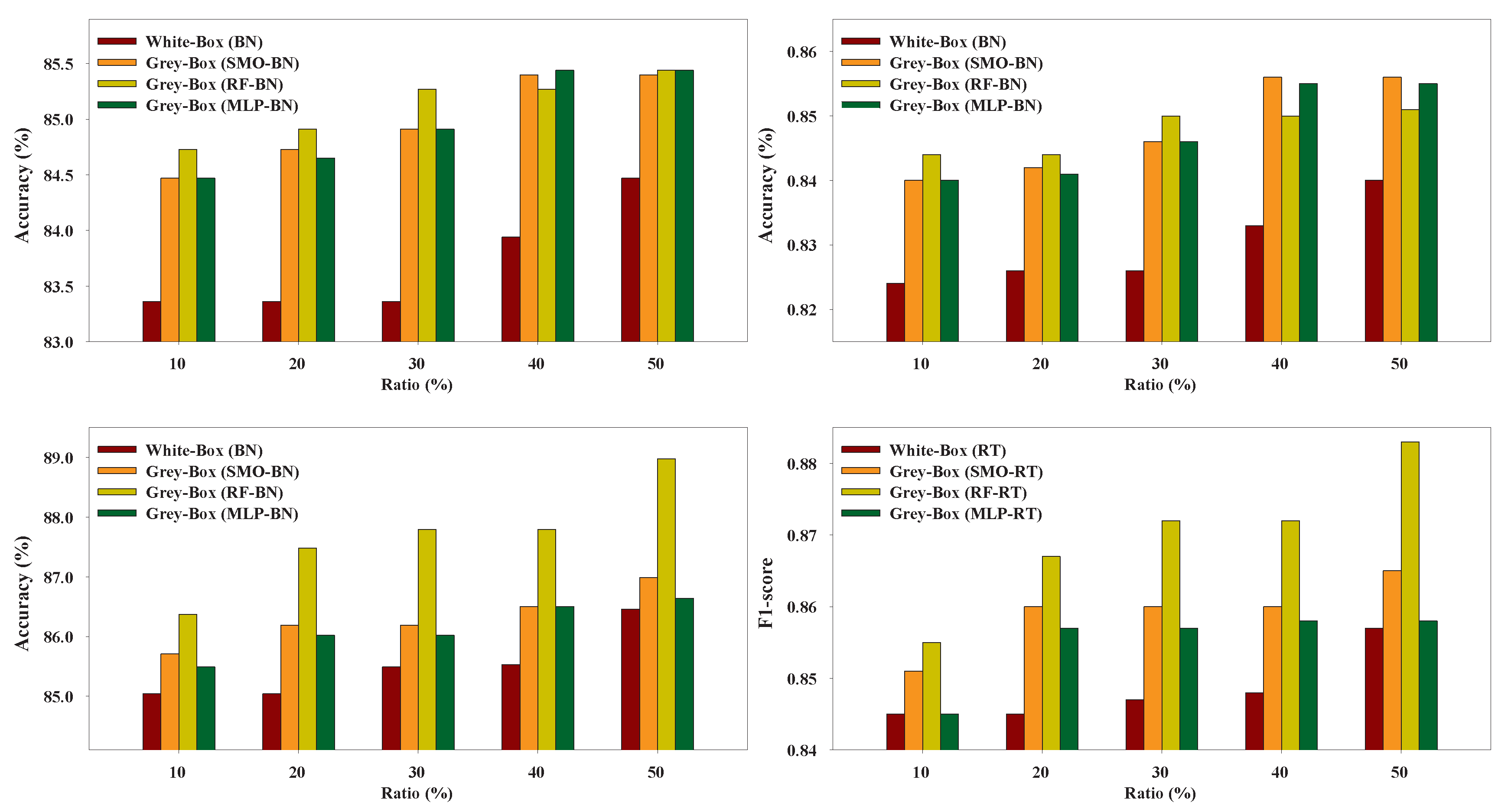
6.1. Grey-Box Models vs. White-Box Models
Figure 3,
Figure 4,
Figure 5,
Figure 6,
Figure 7 and
Figure 8 present the performance of the Grey-Box and White-Box models. Regarding both metrics we can observe that the Grey-Box model outperformed the White-Box model for each Black-Box and White-Box classifier combination in most cases, especially on EduDataA, EduDataAB, and Australian datasets. On Coimbra dataset the two models exhibit almost similar performance, with Grey-Box model being slightly better. On Winsconsin dataset the Grey-Box model reported better performance in general, except for ratio 40 and 50 where the White-Box model outperformed the Grey-Box, utilizing RT as White-Box base learner. The interpretation of
Figure 3,
Figure 4,
Figure 5,
Figure 6,
Figure 7 and
Figure 8 reveals that for EduDataA, EduDataAB and Bank marketing datasets, as ratio value increases, the performance of all models increases too, while on the rest datasets, it seems that we cannot state a similar conclusion. We can also observe that the Grey-Box model performs better in most cases for small ratios (10%, 20%, 30%) while it seems that for higher ratios (40%, 50%) the White-Box exhibits similar performance as the Grey-Box model. Summarizing, we point out that the proposed Grey-Box model performs better for small labeled ratios. Additionally, the Grey-Box (SMO-RT) reported the best overall performance reporting the highest classification accuracy in three out of six datasets, while the Grey-Box reported the best performance utilizing RT as White-Box learner, regarding all utilized ratios.
6.2. Grey-Box Models vs. Black-Box Models
Figure 9,
Figure 10,
Figure 11,
Figure 12,
Figure 13 and
Figure 14 present the performance of the Grey-Box and Black-Box models utilized in our experiments. We can conclude that the Grey-Box model was nearly as accurate as a Black-Box model with the Black-Box being slightly better. More specifically, the Black-Box model clearly outperformed the Grey-Box model on EduDataA and EduDataAB datasets while the Grey-Box reported better performance on Australian dataset. On Bank marketing, Coimbra, and Winsconsin datasets both models exhibited similar performance.
7. Discussion
7.1. Discussion about the Method
In this work, we focus on developing an interpretable and accurate Grey-Box prediction model applied on datasets with a small number of labeled data. For this task, we utilized a Black-Box base learner on a self-training methodology in order to acquire an enlarged labeled dataset which was used for training a White-Box learner. Self-training was considered the most appropriate self-labeled method to use, due to its simplicity, efficiency and because is a widely used single view algorithm [
4]. More specifically, in our proposed framework, an arbitrary classifier is initially trained with a small amount of labeled data, constituting its training set which is iteratively augmented using its own most confident predictions of the unlabeled data. More analytically, each unlabeled instance which has achieved a probability over a specific threshold is considered sufficiently reliable to be added to the labeled training set and subsequently the classifier is retrained. In contrast to the classic self-training framework, we utilized the White-Box learner as the final predictor. Therefore, by training a Black-Box model on the initial labeled data we obtain a larger and a more accurate final labeled dataset, while utilizing a White-Box trained on the final labeled data and being the final predictor, we are able to obtain explainability and interpretability on the final predictions.
In contrast to Grau et al. [
12] approach, we decided to augment the labeled dataset utilizing the most confident predictions from the unlabeled dataset. This way we may lose some extra instances, leading to a smaller final labeled dataset, but instead we manage to avoid mislabeling of new instances and thus reduce the “noise” of the new augmented dataset. Thus, we addressed the weakness of including erroneous labeled instances in the enlarged labeled dataset which could probably lead the White-Box classifier to poor performance.
Che et al. [
19] proposed an interpretable mimic model which falls into the intrinsic interpretability category similar to our proposed model. Nevertheless, the main difference compared to our approach is that we aim to add interpretability on semi supervised algorithms (self-training) which means that our proposed model is mostly recommended on scenarios in which the labeled dataset is limited while a big pool of unlabeled data is available.
7.2. Discussion about the Prediction Accuracy of the Grey-Box Model
In terms of accuracy, our proposed Grey-Box model outperformed White-Box model in most cases of our experiments especially on our educational datasets. As regards, Coimbra dataset, the two models reported almost identical performance with Grey-Box to be slightly better. Relative to Winsconsin dataset there were two cases in which the White-Box model reported better performance over the Grey-Box. Probably this occurs due to the fact that these datasets are very small (few number of labeled instances) and becoming even smaller by the self-training framework as the datasets have to be split in labeled and unlabeled datasets.
Most of Black-Box models are by nature “data-eaters”, especially neural networks, meaning that they need a large number of instances in order to outperform most of White-Box models in terms of accuracy. Our Grey-Box model consists of a Black-Box base learner which was initially trained on the labeled dataset and then makes predictions on the unlabeled data in order to augment the labeled dataset which is then used for training a White-Box learner. If the initial dataset is too small, there is the risk that the Black-Box could exhibit poor performance and make wrong predictions on the unlabeled dataset. This implies that the final augmented dataset will have a lot of mislabeled instances forcing the White-Box, which is the output of the Grey-Box model, to exhibit low performance too. As a result, the proposed Grey-Box model may have lower or equal performance compared to the White-Box model.
Moreover, the Grey–Box model performed slightly worse than the Black-Box models as expected since our goal was to demonstrate that the proposed Grey-Box model achieved a performance almost as good as a Black-Box model. Thus, in summary our results reveal that our model exhibited better performance compared to the White-Box model and reported comparable performance to the Black-Box model.
7.3. Discussion about the Interpretability of the Grey-Box Model
The proposed Grey-Box model falls into the intrinsic interpretability category as its output predictor is a White-Box model and by nature all White-Box models are interpretable. Nevertheless, it does not have the disadvantage of low accuracy inherent to methods of this category as it performs as good as post-hoc methods.
Also, in order to present how the interpretability and explainability of our Grey-Box model comes up in practice, we conducted a case study (experiment example) for the Coimbra dataset utilizing Grey-Box (SMO-RT) because this model exhibited better overall performance. For this task, we made predictions for two instances (persons) utilizing our trained Grey-Box model and now we attempt to explain, in understandable to every human terms, why our model made these predictions.
Table 3 presents the values of each attribute for two instances of the Coimbra dataset while a detailed description of the attributes can be found in [
24].
Figure 15 presents the trained Grey-Box model’s inner structure. From the interpretation of the Grey-Box model, we conclude that the model suggests as the most significant feature, the “age”, since it is in the root of the tree, while we can also observe that a wide range of features are not utilized at all from the model’s inner structure.
Furthermore, by observing the inner structure of the model we can easily extract the model predictions for both instances by just following the nodes and the arrows of the tree, based on the feature values of each person, this procedure is performed, until we reach a leaf of the tree which has the output prediction of the model. More specifically, the Instance1 has “Age = 51” and for the first node the statement “age ≤ 37” is “false”, thus we move right to the next node which has the statement “HOMA ≤ 2.36”. This is “true”, so we move left to “glucose ≤ 91.5” which is “false” since the Instance1 has “glucose = 103”. Therefore, the model’s prediction for the Instance1 is “patient”. By a similar procedure we can extract the model’s prediction for Instance2 which is “healthy”. Next, we can also draw some rules from the model and translate them into explanations such as
Rule 1: “The persons which are of age over 37, have HOMA lower than 2.36, and have glucose over than 91.5, most probably are patients”.
Rule 2: “The persons which are of age lower than 37 and have glucose lower than 91.5 most probably are healthy.”
and so on. Instance1 falls exactly on Rule 1, while Instance2 falls exactly on Rule 2. Thus, an explanation for the Grey–Box model’s predictions could be that Instance1 is probably “patient” because he/she is older than 37 years old and has very low HOMA with high glucose level, while Instance2 is probably “healthy” because he/she is under 37 years old and has low glucose level.
8. Conclusions
In this work, we developed a high performance and interpretable Grey-Box ML model. Our main purpose was to acquire both benefits of black and White-Box models in order to build an interpretable classifier with a better classification performance, compared to a single White-Box model and comparable to that of a Black-Box. More specifically, we utilized a Black-Box model to enlarge an initial labeled dataset and the final augmented dataset was used to train a White-Box model. In contrast to the self-training framework, this trained White-Box model was utilized as the final predictor. This ensemble model falls into the category of intrinsic interpretability since its output predictor is a White-Box which is by nature interpretable. Our experimental results revealed that our proposed Grey-Box model has accuracy comparable to that of a Black-Box but better accuracy comparing to a single White-Box model, being at the same time interpretable as a White-Box model.
In our future work, we aim to extend our experiments of the proposed model to several datasets and improve its prediction accuracy with more sophisticated and theoretically motivated ensemble learning methodologies combining various self-labeled algorithms.


