Image Restoration Using a Fixed-Point Method for a TVL2 Regularization Problem

Abstract

In this paper, we first propose a new TVL2 regularization model for image restoration, and then we propose two iterative methods, which are fixed-point and fixed-point-like methods, using CGLS (Conjugate Gradient Least Squares method) for solving the new proposed TVL2 problem. We also provide convergence analysis for the fixed-point method. Lastly, numerical experiments for several test problems are provided to evaluate the effectiveness of the proposed two iterative methods. Numerical results show that the new proposed TVL2 model is preferred over an existing TVL2 model and the proposed fixed-point-like method is well suited for the new TVL2 model.

1. Introduction

Image restoration is the fundamental problem in image processing that recovers a true image from a blurry and noisy image. The problem of image restoration usually reduces to find the optimal solution $u\in {\mathbb{R}}^m$ based on the following model:

$$f=Au+\epsilon ,$$

(1)

where $A\in {\mathbb{R}}^{m\times m}$ is a blurring operator, $\epsilon \in {\mathbb{R}}^m$ is an unknown white Gaussian noise with variance $\sigma$, and f and u denote the observed degraded image and the original image, respectively. Our purpose is to restore the original image u from blurred and noisy image f as well as possible.

Over the past few decades, optimization techniques and various variation models [1,2,3] have been widely studied and applied in many image processing fields. The well-known ROF (Rudin–Osher–Fatemi) total variation model [3] produces the deblurred image given by the following minimization problem:

$$\underset{u}{min}\left\{\frac{1}{2}{\parallel Au-f\parallel }_2^2+\beta TV(u)\right\},$$

(2)

where $TV(u)$ is the total variation (TV) of u and $\beta >0$ is a regularization parameter.

Many computational methods for solving problem (2) have been proposed in recent years. For example, the time-marching PDE method, the subgradient descent method, the Newton-like method, the second-order cone programming method, the lagged diffusivity fixed-point method, and the split Bregman method have been proposed by many researchers (see [1,3,4,5,6,7,8,9,10,11,12,13] for details).

Recently, Chen et al. [14] proposed a fixed-point method for solving the following constrained TVL2 deblurring problem:

$$\underset{u\in C}{min}\left\{\frac{1}{2}{\parallel Au-f\parallel }_2^2+\frac{\alpha }{2}{\parallel u\parallel }_2^2+\beta TV(u)\right\},$$

(3)

where $\alpha$ and $\beta$ are positive constants, and C is a closed convex subset of ${\mathbb{R}}^{n^2}$. In this paper, we only consider the case for $C={\mathbb{R}}^{n^2}$. That is, we only consider the unconstrained TVL2 problem (3) with $C={\mathbb{R}}^{n^2}$. This approach motivates us to propose a new TVL2 deblurring model

$$\underset{u\in {\mathbb{R}}^{n^2}}{min}\left\{\frac{1}{2}{\parallel Au-f\parallel }_2^2+\alpha {\parallel u\parallel }_2+\beta TV(u)\right\},$$

(4)

where $A\in {\mathbb{R}}^{n^2\times n^2}$ is a blurring matrix, $u\in {\mathbb{R}}^{n^2}$ is an original image, $f\in {\mathbb{R}}^{n^2}$ is a degraded image, $\alpha$ and $\beta$ are positive regularization parameters, and $TV(u)$ stands for the isotropic TV of u. Note that the new TVL2 model (4) uses a non-smooth term ${\parallel u\parallel }_2$ instead of using a smooth term ${\parallel u\parallel }_2^2$ for the purpose of better preserving the edges and corners in the restored images. The isotropic TV of u is defined by

$${\displaystyle TV(u)=\sum _{i=1}^{n^2}\sqrt{{|(\nabla u)}_i^x{|}^2+{\left|{(\nabla u)}_i^y\right|}^2}=\sum _{i=1}^{n^2}{∥\left(\begin{array}{c}{(\nabla u)}_i^x\\ {(\nabla u)}_i^y\end{array}\right)∥}_2,}$$

where the discrete gradient operator $\nabla :{\mathbb{R}}^{n^2}\to {\mathbb{R}}^{2n^2}$ is defined by

$${(\nabla u)}_i=({(\nabla u)}_i^x,{(\nabla u)}_i^y),i=1,2,\cdots ,n^2$$

with

$$\begin{array}{c}\hfill {(\nabla u)}_i^x=\left\{\begin{array}{cc}0\hfill & \mathrm{if}i\mathrm{mod}n=1,\hfill \\ u_i-u_{i-1}\hfill & \mathrm{if}i\mathrm{mod}n\ne 1,\hfill \end{array}\right.\mathrm{and}{(\nabla u)}_i^y=\left\{\begin{array}{cc}0\hfill & \mathrm{if}i\le n,\hfill \\ u_i-u_{i-n}\hfill & \mathrm{if}i>n.\hfill \end{array}\right.\end{array}$$

Notice that TVL2 problems (3) have a unique solution since its objective function is strictly convex, while the new TVL2 problem (4) may not have a unique solution since its objective function is just convex, not strictly convex.

The purpose of this paper is to propose two iterative methods, which are fixed-point and fixed-point-like methods, using CGLS (Conjugate Gradient Least Squares method [15]) for solving the new proposed TVL2 problem (4). This paper is organized as follows. In Section 2, we introduce some definitions and properties that are used in this paper. In Section 3, we first propose a fixed-point method using CGLS for solving TVL2 problem (4), and then we provide convergence analysis for the fixed-point method. In Section 4, we propose a fixed-point-like method using CGLS for solving TVL2 problem (4). In Section 5, we just provide the split Bregman methods for solving TVL2 problems (3) and (4) to see how efficiently the fixed-point and fixed-point-like methods perform. In Section 6, we describe how to carry out numerical experiments for several test problems in order to evaluate the effectiveness of the proposed two iterative methods. This can be done by comparing their performances for TVL2 problem (4) with those of the fixed-point method proposed in [14] for TVL2 problem (3) and the split Bregman methods for TVL2 problems (3) and (4). In Section 7, we provide numerical results for all test problems. Lastly, some conclusions are drawn.

2. Preliminaries

In this section, we briefly refer to some definitions and important properties which will be the foundation for the development of algorithms proposed in this paper.

Definition 1.

Let $\phi :{\mathbb{R}}^n\to \mathbb{R}\cup \{+\infty \}$ be a proper, convex, and lower semi-continuous function (see [16]). The proximity operator of φ at $x\in {\mathbb{R}}^n$ is defined by

$${\mathit{prox}}_{\phi }(x)=\mathit{argmin}\left\{\frac{1}{2}{\parallel u-x\parallel }_2^2+\phi (u):u\in {\mathbb{R}}^n\right\}.$$

(5)

Definition 2.

Let $\phi :{\mathbb{R}}^n\to \mathbb{R}\cup \{+\infty \}$ be a proper, convex, and lower semi-continuous function. The subdifferential of φ at $x\in {\mathbb{R}}^n$ is defined by

$$\partial \phi (x)=\{y\in {\mathbb{R}}^n:\phi (z)\ge \phi (x)+\langle y,z-x\rangle ,\forall z\in {\mathbb{R}}^n\}.$$

(6)

Definition 3.

A nonlinear operator $H:{\mathbb{R}}^n\to {\mathbb{R}}^n$ is called non-expansive if for any $x,y\in {\mathbb{R}}^n$,

$${\parallel H(x)-H(y)\parallel }_2\le {\parallel x-y\parallel }_2.$$

(7)

Definition 4.

A nonlinear operator $H:{\mathbb{R}}^n\to {\mathbb{R}}^n$ is called firmly non-expansive if for any $x,y\in {\mathbb{R}}^n$,

$${\parallel H(x)-H(y)\parallel }_2^2\le \langle x-y,H(x)-H(y)\rangle .$$

(8)

It is easy to show that a firmly non-expansive operator is non-expansive. The following proposition shows a relationship between the proximity operator and the subdifferential of a convex function.

Proposition 1.

If φ is a convex function defined on ${\mathbb{R}}^n$ and $x,y\in {\mathbb{R}}^n$, then (see [16, 17, 18])

$$y\in \partial \phi (x)\iff x={\mathrm{prox}}_{\phi }(x+y).$$

(9)

Let $\phi :{\mathbb{R}}^{2n^2}\to \mathbb{R}$ be a convex function defined by

$${\displaystyle \phi (d)=\sum _{i=1}^{n^2}{∥\left(\begin{array}{c}{d}_i\\ d_{n^2+i}\end{array}\right)∥}_2\mathrm{for}\mathrm{each}d=(d_i)\in {\mathbb{R}}^{2n^2},}$$

(10)

and let B be a $2n^2\times n^2$ matrix that represents a discrete gradient operator ∇, which is

$$B=\left(\begin{array}{c}{I}_n\otimes D\\ D\otimes I_n\end{array}\right),$$

(11)

where $I_n$ is the $n\times n$ identity matrix, ⊗ denotes the Kronecker product, and D is the first order finite difference matrix of order n

$$D=\left(\begin{array}{ccccc}0& 0& \cdots & \cdots & 0\\ -1& 1& \cdots & \cdots & 0\\ ⋮& \ddots & \ddots & \ddots & ⋮\\ 0& \cdots & -1& 1& 0\\ 0& \cdots & 0& -1& 1\end{array}\right).$$

Then, the isotropic TV of $u\in {\mathbb{R}}^{n^2}$ can be expressed as

$$TV(u)=(\phi \circ B)(u).$$

(12)

We now provide the fixed-point method, called Algorithm 1, for solving TVL2 problem (3), which was proposed by Chen et al. [14].

Algorithm 1 Fixed-point method for TVL2 problem (3)

1: Given : observed image f, positive parameters $\alpha ,\beta ,\lambda$ and $\kappa \in (0,1)$ 2: Initialization : $v^0=0$ and $u^0=f$ 3: for$k=0$ to $maxit$ do 4:  Solve $(A^{T}A+\alpha I)u^{k+1}=A^{T}f-\lambda B^T{v}^k$ for $u^{k+1}$ 5:  $v^{k+1}=\kappa v^k+(1-\kappa )(I-{\mathrm{prox}}_{\frac{\beta }{\lambda }\phi })(v^k+B{u}^{k+1})$ 6:  if $\frac{\parallel u^{k+1}-u^k{\parallel }_2}{\parallel u^{k+1}{\parallel }_2}<tol$ then 7:   Stop 8:  end if 9: end for

Notice that line 4 of Algorithm 1 is solved using CGLS instead of using CG (Conjugate Gradient method [19,20,21]) since the linear system in line 4 is equivalent to solving the following least squares problem

$$\underset{u}{min}{∥\left(\begin{array}{c}f\\ -\frac{\lambda }{\sqrt{\alpha }}{B}^T{v}^k\end{array}\right)-\left(\begin{array}{c}A\\ \sqrt{\alpha }I\end{array}\right)u∥}_2^2.$$

For all algorithms presented in this paper, maxit denotes the maximum number of iterations, and tol denotes the tolerance value of the stopping criterion.

3. Fixed-Point Method for TVL2 Problem (4)

In this section, we propose a fixed-point method using CGLS for solving the new TVL2 regularization problem (4). From relation (12), TVL2 problem (4) can be expressed as

$$\underset{u\in {\mathbb{R}}^{n^2}}{min}\left\{\frac{1}{2}{\parallel Au-f\parallel }_2^2+\alpha {\parallel u\parallel }_2+\beta (\phi \circ B)(u)\right\}.$$

(13)

Using Proposition 1, we can obtain the following property for a solution of TVL2 problem (13).

Theorem 1.

If φ is a real valued convex function on ${\mathbb{R}}^{2n^2}$, B is a $2n^2\times n^2$ matrix, A is an $n^2\times n^2$ matrix, u is a solution to model (13), then, for any $\gamma ,\lambda >0$ there exist vectors $a\in {\mathbb{R}}^{n^2}$ and $b\in {\mathbb{R}}^{2n^2}$ such that

$$\begin{array}{cc}\hfill & a=(I-{\mathrm{prox}}_{\frac{1}{\gamma }{\parallel ·\parallel }_2})(u+a),\hfill \end{array}$$

(14)

$$\begin{array}{cc}\hfill & b=(I-{\mathrm{prox}}_{\frac{\beta }{\lambda }\phi })(Bu+b),\hfill \end{array}$$

(15)

$$\begin{array}{cc}\hfill & (A^{T}A)u=A^{T}f-\alpha \gamma a-\lambda B^{T}b.\hfill \end{array}$$

(16)

Conversely, if there exists $\gamma ,\lambda >0,a\in {\mathbb{R}}^{n^2}$, $b\in {\mathbb{R}}^{2n^2}$ and $u\in {\mathbb{R}}^{n^2}$ satisfying Equations (14)–(16), then u is a solution to model (13).

Proof. 

Assume that $u\in {\mathbb{R}}^{n^2}$ is a solution to the model (13). By Fermat’s rule in convex analysis for model (13), we obtain the following equivalent relation for the solution u

$$\begin{array}{cc}\hfill 0& \in A^T{(Au-f)+\alpha ·\partial (\parallel ·\parallel }_2)(u)+\beta B^T\circ (\partial \phi )\circ (Bu)\hfill \\ \hfill & =A^T{(Au-f)+\alpha ·\partial (\parallel ·\parallel }_2)(u)+B^T\partial (\beta \phi )(Bu).\hfill \end{array}$$

(17)

For any $\gamma ,\lambda >0$, we can choose two vectors $a\in \partial (\frac{1}{\gamma }\parallel ·{\parallel }_2)(u)$ and $b\in \partial (\frac{\beta }{\lambda }\phi )(Bu)$ satisfying

$$A^T(Au-f)+\alpha \gamma a+\lambda B^{T}b=0.$$

(18)

Using Proposition 1, one obtains

$$u={\mathrm{prox}}_{\frac{1}{\gamma }{\parallel ·\parallel }_2}(u+a)\mathrm{and}Bu={\mathrm{prox}}_{\frac{\beta }{\lambda }\phi }(Bu+b).$$

(19)

From Equation (19), we obtain Equations (14) and (15). In addition, from Equation (18), we obtain Equation (16).

Conversely, suppose that there exist $\gamma ,\lambda >0,a,b$ and $u\in {\mathbb{R}}^{n^2}$ satisfying Equations (14)–(16). From Equation (16), we obtain Equation (18). By Proposition 1, Equations (14) and (15) ensure $a\in \partial (\frac{1}{\gamma }\parallel ·{\parallel }_2)(u)$ and $b\in \partial (\frac{\beta }{\lambda }\phi )(Bu)$, respectively. Using these relations and Equation (18), one obtains

$$\begin{array}{cc}\hfill 0& =A^T(Au-f)+\alpha \gamma a+\lambda B^{T}b\hfill \\ \hfill & \in A^T{(Au-f)+\alpha \partial (\parallel ·\parallel }_2)(u)+\beta B^T\circ (\partial \phi )\circ (Bu).\hfill \end{array}$$

Consequently, Equation (17) holds. Thus, u is a solution to model (13). □

From Equations (14)–(16) in Theorem 1, we can develop a fixed-point algorithm which converges to a solution to TVL2 problem (4). We now describe how to develop the fixed-point algorithm. Let u be an approximate solution to the ill-conditioned linear system (16) in Theorem 1. Then, u can be expressed as

$$u=M(A^{T}f-\alpha \gamma a-\lambda B^{T}b),$$

(20)

where M is a symmetric positive semi-definite matrix approximating an inverse of the linear system matrix in (16). For example, we can choose $M={(A^{T}A)}_r^{†}$, which is a truncated pseudoinverse of $A^{T}A$ using the r largest positive singular values of $A^{T}A$. Substituting Equation (20) into Equations (14) and (15), one obtains

$$\begin{array}{c}a=(I-{\mathrm{prox}}_{\frac{1}{\gamma }{\parallel ·\parallel }_2})\left((I_{n^2}-\alpha \gamma M)a-\lambda M{B}^{T}b+M{A}^{T}f\right),\hfill \end{array}$$

(21)

$$\begin{array}{c}b=(I-{\mathrm{prox}}_{\frac{\beta }{\lambda }\phi })\left(-\alpha \gamma BMa+(I_{2n^2}-\lambda BM{B}^T)b+BM{A}^{T}f\right).\hfill \end{array}$$

(22)

Let us define some operators. For the given convex functions $\frac{1}{\gamma }{\parallel ·\parallel }_2$ on ${\mathbb{R}}^{n^2}$ and $\frac{\beta }{\lambda }\phi$ on ${\mathbb{R}}^{2n^2}$, we define an operator $T:{\mathbb{R}}^{3n^2}\to {\mathbb{R}}^{3n^2}$ at a vector $\left(\genfrac{}{}{0pt}{}{u}{v}\right)\in {\mathbb{R}}^{3n^2}$ with $u\in {\mathbb{R}}^{n^2}$ and $v\in {\mathbb{R}}^{2n^2}$ as follows:

$$T\left(\genfrac{}{}{0pt}{}{u}{v}\right)=\left(\begin{array}{c}(I-{\mathrm{prox}}_{\frac{1}{\gamma }{\parallel ·\parallel }_2})(u)\\ (I-{\mathrm{prox}}_{\frac{\beta }{\lambda }\phi })(v)\end{array}\right).$$

(23)

We also introduce an affine transformation $L:{\mathbb{R}}^{3n^2}\to {\mathbb{R}}^{3n^2}$ defined, for all $\left(\genfrac{}{}{0pt}{}{a}{b}\right)\in {\mathbb{R}}^{3n^2}$ with $a\in {\mathbb{R}}^{n^2}$ and $b\in {\mathbb{R}}^{2n^2}$, by

$$L\left(\genfrac{}{}{0pt}{}{a}{b}\right)=\left(\begin{array}{cc}{I}_{n^2}-\alpha \gamma M& -\lambda M{B}^T\\ -\alpha \gamma BM& I_{2n^2}-\lambda BM{B}^T\end{array}\right)\left(\genfrac{}{}{0pt}{}{a}{b}\right)+\left(\begin{array}{c}M{A}^{T}f\\ BM{A}^{T}f\end{array}\right),$$

(24)

and an operator $G:{\mathbb{R}}^{3n^2}\to {\mathbb{R}}^{3n^2}$ defined by

$$G=T\circ L.$$

(25)

Then, Equations (21) and (22) can be expressed as

$$w=Gw,$$

(26)

where $w=\left(\genfrac{}{}{0pt}{}{a}{b}\right)$.

Proposition 2.

The operator G defined by (25) has a fixed point.

Proof. 

Since a solution of TVL2 problem (13) exists, from Equation (26) and the first part of the proof of Theorem 1, G has a fixed point. □

Lemma 1.

If the operator T is defined by Equation (23), then the operator T is non-expansive.

Proof. 

Note that $I-{\mathrm{prox}}_{\frac{1}{\gamma }{\parallel ·\parallel }_2}$ and $I-{\mathrm{prox}}_{\frac{\beta }{\lambda }\phi }$ are firmly non-expansive and thus non-expansive [7]. For any vectors $s=\left(\genfrac{}{}{0pt}{}{u}{v}\right)\in {\mathbb{R}}^{3n^2}$ and $t=\left(\genfrac{}{}{0pt}{}{a}{b}\right)\in {\mathbb{R}}^{3n^2}$ with $u,a\in {\mathbb{R}}^{n^2}$ and $v,b\in {\mathbb{R}}^{2n^2}$

$$\begin{array}{cc}\hfill {\parallel T(s)-T(t)\parallel }_2^2& ={∥\left(\begin{array}{c}(I-{\mathrm{prox}}_{\frac{1}{\gamma }{\parallel ·\parallel }_2})(u)-(I-{\mathrm{prox}}_{\frac{1}{\gamma }{\parallel ·\parallel }_2})(a)\\ (I-{\mathrm{prox}}_{\frac{\beta }{\lambda }\phi })(v)-(I-{\mathrm{prox}}_{\frac{\beta }{\lambda }\phi })(b)\end{array}\right)∥}_2^2\hfill \\ \hfill & ={∥(I-{\mathrm{prox}}_{\frac{1}{\gamma }{\parallel ·\parallel }_2})(u)-(I-{\mathrm{prox}}_{\frac{1}{\gamma }{\parallel ·\parallel }_2})(a)∥}_2^2\hfill \\ \hfill & +{∥(I-{\mathrm{prox}}_{\frac{1}{\gamma }{\parallel ·\parallel }_2})(v)-(I-{\mathrm{prox}}_{\frac{1}{\gamma }{\parallel ·\parallel }_2})(b)∥}_2^2\hfill \\ \hfill & \le {\parallel u-a\parallel }_2^2+{\parallel v-b\parallel }_2^2\hfill \\ \hfill & ={∥\left(\begin{array}{c}u-a\\ v-b\end{array}\right)∥}_2^2={\parallel s-t\parallel }_2^2.\hfill \end{array}$$

Hence, one obtains ${\parallel T(s)-T(t)\parallel }_2\le {\parallel s-t\parallel }_2$, which means that the operator T is non-expansive. □

Let

$$c:=\left(\begin{array}{c}M{A}^{T}f\\ BM{A}^{T}f\end{array}\right)\in {\mathbb{R}}^{3n^2},P:=\left(\begin{array}{c}{I}_{n^2}\\ B\end{array}\right),R:=\left(\begin{array}{cc}\alpha \gamma I_{n^2}& 0\\ 0& \lambda I_{2n^2}\end{array}\right).$$

Then, Label (24) can be expressed as

$$Lw=(I_{3n^2}-PM{P}^{T}R)w+c.$$

(27)

Proposition 3.

If φ is a convex function on ${\mathbb{R}}^{2n^2}$, B is a $2n^2\times n^2$ matrix, A is an $n^2\times n^2$ matrix and $\alpha ,\gamma ,\lambda$ are positive constants such that $\parallel I_{3n^2}-PM{P}^T{R\parallel }_2\le 1$, then G is non-expansive.

Proof. 

Since the operator T is non-expansive by Lemma 1, for all $w_1,w_2\in {\mathbb{R}}^{3n^2}$, we have

$$\begin{array}{cc}\hfill \parallel G(w_1)-G(w_2){\parallel }_2& =\parallel T(L{w}_1)-T(L{w}_2){\parallel }_2\hfill \\ \hfill & \le \parallel L{w}_1-L{w}_2{\parallel }_2.\hfill \end{array}$$

By the assumption $\parallel I_{3n^2}-PM{P}^T{R\parallel }_2\le 1$ and Equation (27), we obtain

$$\begin{array}{cc}\hfill \parallel L{w}_1-L{w}_2{\parallel }_2& =\parallel (I_{3n^2}-PM{P}^{T}R)(w_1-w_2){\parallel }_2\hfill \\ \hfill & \le \parallel I_{3n^2}-PM{P}^T{R\parallel }_2{\parallel w_1-w_2\parallel }_2\hfill \\ \hfill & \le \parallel w_1-w_2{\parallel }_2.\hfill \end{array}$$

Hence, G is non-expansive. □

Let $S:{\mathbb{R}}^N\to {\mathbb{R}}^N$ be an operator. Then, the Picard iteration of the operator S is defined by

$$x_{i+1}=S{x}_i(i=0,1,2,\cdots )$$

for a given vector $x_0\in {\mathbb{R}}^N$. For $\kappa \in (0,1)$, the $\kappa$-averaged operator $S_{\kappa }$ of S is defined by

$$S_{\kappa }=\kappa I+(1-\kappa )S.$$

Proposition 4

(Optial $\kappa$-averaged Theorem). Let C be a closed convex set in ${\mathbb{R}}^{3n^2}$ and let $S:C\to C$ be a non-expansive mapping with at least one fixed point. Then, for any $w^0\in C$ and $\kappa \in (0,1)$, the Picard iteration of $S_{\kappa }$ converges to a fixed point of S (see [22]).

Theorem 2.

If φ is a convex function, A is an $n^2\times n^2$ matrix, B is a $2n^2\times n^2$ matrix and $\alpha ,\gamma ,\lambda >0$ are positive constants such that $\parallel I_{3n^2}-PM{P}^T{R\parallel }_2\le 1$, then for any $\kappa \in (0,1)$ the Picard iteration of $G_{\kappa }$ converges to a fixed point of G.

Proof. 

From Propositions 2 and 3, we know that the opertor G has a fixed point and is non-expansive. Hence, for any $w^0\in {\mathbb{R}}^{3n^2}$ and $\kappa \in (0,1)$, the Picard iteration of $G_{\kappa }$ converges to a fixed point of G by Proposition 4. □

For a square matrix K, let $\rho (K)$ denote the spectral radius of K. Then, the following lemma can be obtained.

Lemma 2.

Let φ and B be defined by Equations (10) and (11) respectively, and let A be a given $n^2\times n^2$ blurring matrix. If we choose $\alpha ,\gamma$ and λ such that

$$0<\lambda =\alpha \gamma <\frac{2}{\rho (PM{P}^T)},$$

then $\parallel I_{3n^2}-PM{P}^T{R\parallel }_2\le 1$ and thus the operator G is non-expansive.

Proof. 

Since $\lambda =\alpha \gamma$ and thus $R=\lambda I_{3n^2}$, one obtains

$$I_{3n^2}-PM{P}^{T}R=I_{3n^2}-\lambda PM{P}^T.$$

Note that $PM{P}^T$ is a symmetric positive semi-definite matrix. Hence,

$$\begin{array}{cc}\hfill \parallel I_{3n^2}-PM{P}^T{R\parallel }_2& =\rho (I_{3n^2}-\lambda PM{P}^T)\hfill \\ \hfill & =\max \left\{\right|1-\lambda ·{\lambda }_{\min }(PM{P}^T)|,|1-\lambda ·{\lambda }_{\max }(PM{P}^T)\left|\right\},\hfill \end{array}$$

where ${\lambda }_{\min }(PM{P}^T)$ and ${\lambda }_{\max }(PM{P}^T)$ denote the minimum and maximaum eigenvalues of $PM{P}^T$, respectively. Since $0<\lambda =\alpha \gamma <\frac{2}{\rho (PM{P}^T)}$, $0\le \lambda ·{\lambda }_{\min }(PM{P}^T)<2$ and $0<\lambda ·{\lambda }_{\max }(PM{P}^T)<2$. Hence, one obtains

$$\parallel I_{3n^2}-PM{P}^T{R\parallel }_2\le 1.$$

Therefore, the operator G is non-expansive by Proposition 3. □

Theorem 3.

If the assumptions of Lemma 2 hold and $\kappa \in (0,1)$, then the Picard iteration of $G_k$ converges to a fixed point of G.

Proof. 

The proof follows from Lemma 2 and Theorem 2. □

From Theorem 2 and the Picard iteration of the $\kappa$-averaged operator $G_{\kappa }=\kappa I+(1-\kappa )G$, we can obtain a fixed-point method, called Algorithm 2, which converges to a solution to TVL2 problem (4).

Algorithm 2 Fixed-point method for TVL2 problem (4)

1: Given : observed image f, positive parameters $\alpha ,\beta ,\gamma ,\lambda$ and $\kappa \in (0,1)$ 2: Initialization : $a^0=0$, $b^0=0$ and $u^0=f$ 3: for$k=0$ to $maxit$ do 4:  ${\widehat{a}}^{k+1}=\left(I-{\mathrm{prox}}_{\frac{1}{\gamma }{\parallel ·\parallel }_2}\right)\left(u^k+a^k\right)$ 5:  $a^{k+1}=\kappa a^k+(1-\kappa ){\widehat{a}}^{k+1}$ 6:  ${\widehat{b}}^{k+1}=\left(I-{\mathrm{prox}}_{\frac{\beta }{\lambda }\phi }\right)\left(B{u}^k+b^k\right)$ 7:  $b^{k+1}=\kappa b^k+(1-\kappa ){\widehat{b}}^{k+1}$ 8:  Solve $A^{T}A{u}^{k+1}=A^{T}f-\alpha \gamma a^{k+1}-\lambda B^T{b}^{k+1}$ for $u^{k+1}$ 9:  if $\frac{\parallel u^{k+1}-u^k{\parallel }_2}{\parallel u^{k+1}{\parallel }_2}$ < tol then 10:   Stop 11:  end if 12: end for

The linear system in line 8 of Algorithm 2 is ill-conditioned, so we need to consider how to find an approximate solution to the ill-conditioned linear system. A typical method for finding an approximate solution to the linear system is

$$u^{k+1}=M(A^{T}f-\alpha \gamma a^{k+1}-\lambda B^T{b}^{k+1}),$$

where $M={(A^{T}A)}_r^{†}$. However, computation of ${(A^{T}A)}_r^{†}$ is very time-consuming when A is large. Thus, we want to propose a different approach for finding an approximate solution to the linear system in line 8 of Algorithm 2. We first split the coefficient matrix $A^{T}A$ into

$$A^{T}A=(A^{T}A+\delta D)-(\delta D),$$

(28)

where $\delta$ is a positive constant and $D=\mathrm{d}iag(A^{T}A)$ is a diagonal part of $A^{T}A$. Then, the ill-conditioned linear system can be solved using the following iterative method:

Inner Solver

Choose $y_1=u^k$

for $\ell =1$ to $maxl$

Solve $(A^{T}A+\delta D)y_{\ell +1}=\delta D{y}_{\ell }+A^{T}f-\alpha \gamma a^{k+1}-\lambda B^T{b}^{k+1}$ for $y_{\ell +1}$

end for

$u^{k+1}=y_{\ell +1}$,

where $u^k$ refers to the restored image computed at the previous kth step, and the optimal parameter $\delta >0$ is chosen by numerical tries. Semi-convergence analysis for Inner Solver has been studied by Han and Yun [23]. Algorithm 2 is an iterative method that converges to a solution to TVL2 problem (4) as $k\to \infty$, so we do not have to get an accurate solution to the linear system in line 8 of Algorithm 2. For this reason, we have used $maxl=1$ for Inner Solver.

Notice that the linear system in Inner Solver is equivalent to solving the following least squares problem:

$$\underset{u}{min}{∥\left(\begin{array}{c}f\\ \frac{1}{\sqrt{\delta }}{D}^{-\frac{1}{2}}(\delta D{y}_{\ell }-\alpha \gamma a^{k+1}-\lambda B^T{b}^{k+1})\end{array}\right)-\left(\begin{array}{c}A\\ \sqrt{\delta }{D}^{\frac{1}{2}}\end{array}\right)u∥}_2^2.$$

(29)

Hence, the linear system in Inner Solver is solved by applying the CGLS to (29).

4. Fixed-Point-like Method for TVL2 Problem (4)

In this section, we propose a fixed-point-like method using CGLS for solving the new TVL2 problem (4) that can be obtained by modifying Algorithm 2. Notice that Algorithm 2 computes ${\widehat{a}}^{k+1}$ and $a^{k+1}$ before the solution step of finding $u^{k+1}$ (see lines 4 and 5 of Algorithm 2). However, the fixed-point-like method to be proposed in this section computes ${\widehat{a}}^{k+1}$ and $a^{k+1}$ after the solution step of finding $u^{k+1}$. Below, we describe how to develop the fixed-point-like method in detail. We first split line 4 of Algorithm 2 into

$${\widehat{a}}^{k+1}=u^k+a^{k+\frac{1}{2}},$$

(30)

where $a^{k+\frac{1}{2}}=a^k-{\mathrm{prox}}_{\frac{1}{\gamma }{\parallel ·\parallel }_2}\left(u^k+a^k\right)$. Replacing the old value $u^k$ of Equation (30) with the new value $u^{k+1}$, one obtains the following equation:

$${\widehat{a}}^{k+1}=u^{k+1}+a^{k+\frac{1}{2}}.$$

(31)

Then, the solution step (i.e., line 8 of Algorithm 2) is changed to

$$A^{T}A{u}^{k+1}=A^{T}f-\alpha \gamma {\widehat{a}}^{k+1}-\lambda B^T{b}^{k+1},$$

(32)

where ${\widehat{a}}^{k+1}$ is computed using Equation (31) instead of using Equation (30). Substituting Equation (31) into Equation (32), one obtains

$$(A^{T}A+\alpha \gamma I)u^{k+1}=A^{T}f-\alpha \gamma a^{k+\frac{1}{2}}-\lambda B^T{b}^{k+1}.$$

(33)

After finding $u^{k+1}$ from Equation (33), we compute ${\widehat{a}}^{k+1}$ using Equation (31) and $a^{k+1}=\kappa a^k+(1-\kappa ){\widehat{a}}^{k+1}$. By incorporating the above ideas into Algorithm 2, we can obtain a fixed-point-like method, called Algorithm 4, for solving TVL2 problem (4).

In addition, notice that the linear system in line 7 of Algorithm 3 is equivalent to solving the following least squares problem:

$$\underset{u}{min}{∥\left(\begin{array}{c}f\\ -\frac{1}{\sqrt{\alpha \gamma }}(\alpha \gamma a^{k+\frac{1}{2}}+\lambda B^T{b}^{k+1})\end{array}\right)-\left(\begin{array}{c}A\\ \sqrt{\alpha \gamma }I\end{array}\right)u∥}_2^2.$$

(34)

Hence, the linear system in line 7 of Algorithm 3 is solved using the CGLS instead of using the CG.

Algorithm 3 Fixed-point-like method for TVL2 problem (4)

1: Given : observed image f, positive parameters $\alpha ,\beta ,\gamma ,\lambda$ and $\kappa \in (0,1)$ 2: Initialization : $a^0=0$, $b^0=0$ and $u^0=f$ 3: for$k=0$ to $maxit$ do 4:  $a^{k+\frac{1}{2}}=a^k-{\mathrm{prox}}_{\frac{1}{\gamma }{\parallel ·\parallel }_2}\left(u^k+a^k\right)$ 5:  ${\widehat{b}}^{k+1}=\left(I-{\mathrm{prox}}_{\frac{\beta }{\lambda }\phi }\right)\left(B{u}^k+b^k\right)$ 6:  $b^{k+1}=\kappa b^k+(1-\kappa ){\widehat{b}}^{k+1}$ 7:  Solve $(A^{T}A+\alpha \gamma I)u^{k+1}=A^{T}f-\alpha \gamma a^{k+\frac{1}{2}}-\lambda B^T{b}^{k+1}$ for $u^{k+1}$ 8:  ${\widehat{a}}^{k+1}=u^{k+1}+a^{k+\frac{1}{2}}$ 9:  $a^{k+1}=\kappa a^k+(1-\kappa ){\widehat{a}}^{k+1}$ 10:  if $\frac{\parallel u^{k+1}-u^k{\parallel }_2}{\parallel u^{k+1}{\parallel }_2}<tol$ then 11:   Stop 12:  end if 13: end for

5. Split Bregman Methods for TVL2 Problems (3) and (4)

In this section, we just provide the alternating split Bregman methods for solving the TVL2 problems (3) and (4) in order to evaluate the performance of Algorithms 2 and 3. For more details about the alternating split Bregman method as well as its convergence analysis, we refer to [5,8]. The following Algorithms 4 and 5 are the alternating split Bregman methods corresponding to the TVL2 problems (3) and (4), respectively.

As was done in line 7 of Algorithm 3, the linear systems in line 4 of Algorithms 4 and 5 are solved using the CGLS instead of using the CG.

Algorithm 4 Split Bregman method for TVL2 problem (3)

1: Given : observed image f, positive parameters $\alpha ,\beta ,\lambda$ 2: Initialization : $a^0=0$, $b^0=0$ and $u^0=f$ 3: for$k=0$ to $maxit$ do 4:  Solve $(A^{T}A+\lambda B^{T}B+\alpha I)u^{k+1}=A^{T}f+\lambda B^T(a^k-b^k)$ for $u^{k+1}$ 5:  $a^{k+1}={\mathrm{prox}}_{\frac{\beta }{\lambda }\phi }(B{u}^{k+1}+b^k)$ 6:  $b^{k+1}=b^k+B{u}^{k+1}-a^{k+1}$ 7:  if $\frac{\parallel u^{k+1}-u^k{\parallel }_2}{\parallel u^{k+1}{\parallel }_2}<tol$ then 8:   Stop 9:  end if 10: end for

Algorithm 5 Split Bregman method for TVL2 problem (4)

1: Given : observed image f, positive parameters $\alpha ,\beta ,\lambda ,\gamma$ 2: Initialization : $a^0=b^0=0$, $c^0=d^0=0$ and $u^0=f$ 3: for$k=0$ to $maxit$ do 4:  Solve $(A^{T}A+\lambda B^{T}B+\gamma I)u^{k+1}=A^{T}f+\lambda B^T(d^k-c^k)+\gamma (a^k-b^k)$ for $u^{k+1}$ 5:  $a^{k+1}={\mathrm{prox}}_{\frac{\alpha }{\gamma }{\parallel ·\parallel }_2}(u^{k+1}+b^k)$ 6:  $d^{k+1}={\mathrm{prox}}_{\frac{\beta }{\lambda }\phi }(B{u}^{k+1}+c^k)$ 7:  $b^{k+1}=b^k+u^{k+1}-a^{k+1}$ 8:  $c^{k+1}=c^k+B{u}^{k+1}-d^{k+1}$ 9:  if $\frac{\parallel u^{k+1}-u^k{\parallel }_2}{\parallel u^{k+1}{\parallel }_2}<tol$ then 10:   Stop 11:  end if 12: end for

6. Numerical Experiments

In this section, we describe how to carry out numerical experiments for several test problems to evaluate the efficiency of two iterative methods, called Algorithms 2 and 3, using CGLS for solving the new proposed TVL2 problem (4). Performance of Algorithms 2 and 3 is evaluated by comparing their numerical results with those of the existing fixed-point method called Algorithm 1 and the split Bregman methods called Algorithms 4 and 5.

All numerical tests have been performed using Matlab R2016a on a personal computer equipped with Intel Core i5-3337 1.8 GHz CPU and 8 GB RAM. For numerical experiments, we have used three types of PSFs (point spread functions) which are Gaussian blur with standard deviation 9 and Average blur and Motion blur of size $9\times 9$. PSF arrays P for Gaussian blur with standard deviation 9 and Average blur and Motion blur of size $9\times 9$ are generated by the built-in Matlab function $fspecial({}^{\prime }Gaussia{n}^{\prime },[9,9],9)$, $fspecial({}^{\prime }averag{e}^{\prime },9)$ and

$$P=zeros(9);P(4:6,:)=fspecial({}^{\prime }motio{n}^{\prime },9,1),$$

respectively. The blurred and noisy image f is generated by

$$f=A·vec(X)+vec(E),$$

where A stands for the blurring matrix that can be generated by the PSF array P according to the reflexive boundary condition, and E is the Gaussian white noise with mean 0 and standard deviation 3 that can generated using Matlab function $E=3\times randn(m,n)$, where $(m,n)$ denotes the size of true image.

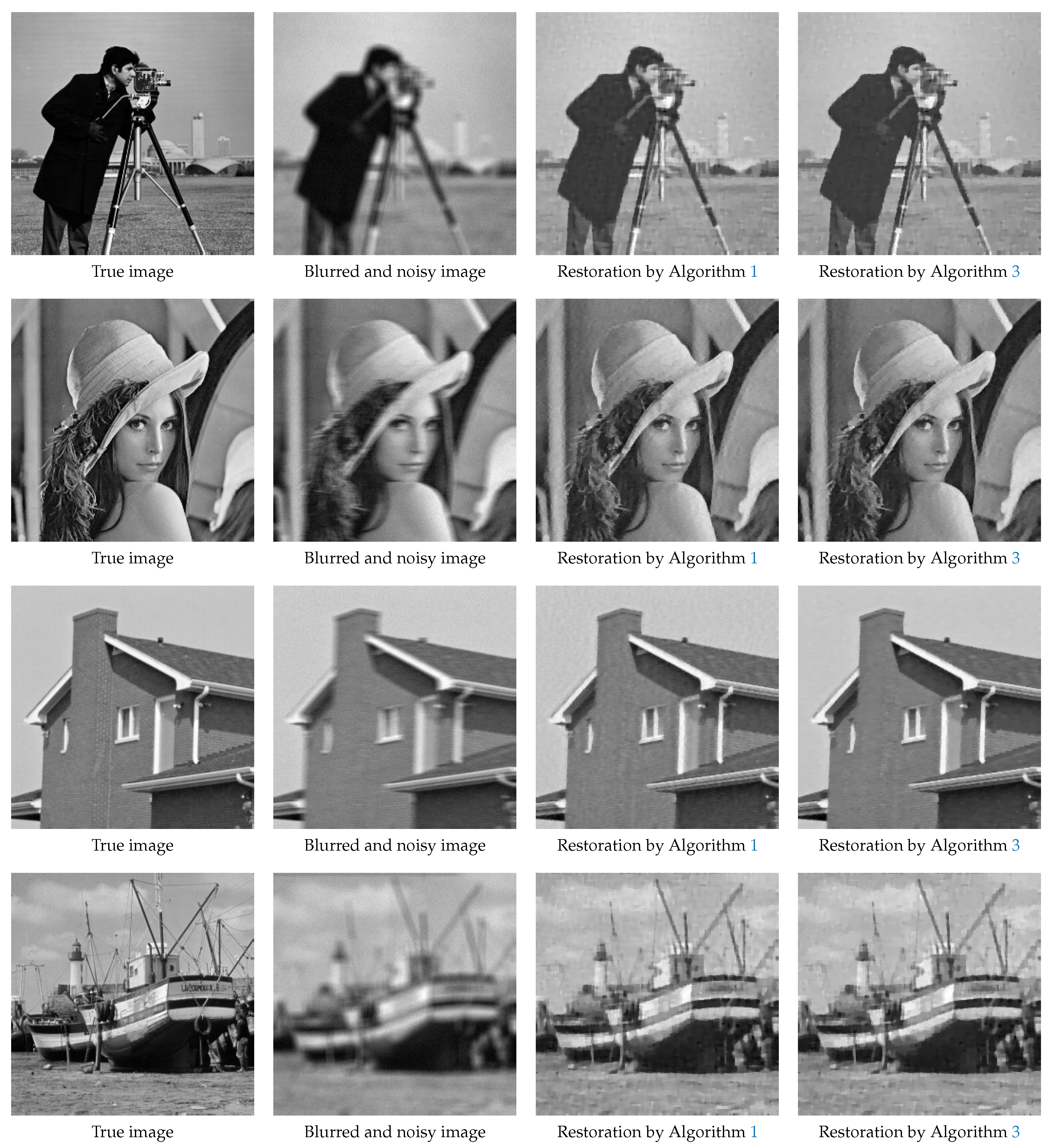
In order to illustrate efficiency of the proposed algorithms, we have used four test images with an intensity range of $[0,255]$ such as Cameraman, Lena, House, and Boat with pixel size $256\times 256$. To evaluate the quality of the restored images, we have used the peak signal-to-noise ratio (PSNR) between the original image and restored image, which is defined by

$$\mathrm{PSNR}=10{\log }_{10}\left(\frac{{\max }_{i,j}{\left|u_{ij}\right|}^2·m·n}{\parallel u-\tilde{u}{\parallel }_F^2}\right),$$

where ${\parallel ·\parallel }_F$ represents the Frobenius norm, $\tilde{u}$ denotes the restored image of the original image u with size $m\times n$, and $u_{ij}$ stands for the value of the original image u at the pixel point $(i,j)$. In general, the larger PSNR stands for the better quality of the restored image.

For all numerical experiments, an initial image was set to the blurred and noisy image f, $\kappa =1\times {10}^{-6}$, $maxit=150$, and $tol$ is set to $5\times {10}^{-4}$ (for Algorithms 1 and 5), $2\times {10}^{-4}$ (for Algorithm 4) or $1\times {10}^{-3}$ (for Algorithms 2 and 3). For the CGLS method that is used to solve a linear system every iteration of Algorithms 1–5, the tolerance for stopping criterion is set to $5\times {10}^{-2}$ (for Algorithms 1, 4 and 5) or $1\times {10}^{-3}$ (for Algorithms 2 and 3), and the maximum number of iterations is set to 60.

7. Numerical Results

In this section, we provide numerical results for four test images that are listed in

Table 1. Numerical results for Cameraman image.

Blur	${\mathbf{P}}_0$	Alg	$\mathit{\alpha }$	$\mathit{\beta }$	$\mathit{\gamma }$	$\mathit{\lambda }$	$\mathit{\delta }$	$\mathit{tol}$	PSNR	Iter
Gaussian	20.85	1	0.0016	0.12		0.00041		$5\times {10}^{-4}$	25.17	67(47)
		2	1.15	0.135	0.05	0.01	4.2	$1\times {10}^{-3}$	24.60	34(9)
		3	1.15	0.135	0.05	0.01		$1\times {10}^{-3}$	25.51	132(8)
		4	0.00001	0.135		0.02		$2\times {10}^{-4}$	25.53	56(10)
		5	0.15	0.14	0.005	0.008		$5\times {10}^{-4}$	25.52	28(13)
Average	20.76	1	0.0016	0.13		0.00041		$5\times {10}^{-4}$	25.24	58(48)
		2	0.75	0.14	0.095	0.0095	4.2	$1\times {10}^{-3}$	24.64	33(9)
		3	0.75	0.14	0.095	0.0095		$1\times {10}^{-3}$	25.59	120(8)
		4	0.00001	0.145		0.02		$2\times {10}^{-4}$	25.60	42(14)
		5	0.01	0.14	0.002	0.009		$5\times {10}^{-4}$	25.61	27(15)
Motion	21.85	1	0.0017	0.22		0.00049		$5\times {10}^{-4}$	28.05	51(36)
		2	0.85	0.23	0.085	0.002	1.3	$1\times {10}^{-3}$	27.52	41(7)
		3	0.85	0.23	0.085	0.002		$1\times {10}^{-3}$	28.57	67(12)
		4	0.00001	0.24		0.03		$2\times {10}^{-4}$	28.51	36(7)
		5	0.01	0.24	0.03	0.003		$5\times {10}^{-4}$	28.59	37(10)

,

Table 2. Numerical results for Lena image.

Blur	${\mathbf{P}}_0$	Alg	$\mathit{\alpha }$	$\mathit{\beta }$	$\mathit{\gamma }$	$\mathit{\lambda }$	$\mathit{\delta }$	$\mathit{tol}$	PSNR	Iter
Gaussian	22.55	1	0.0016	0.17		0.0004		$5\times {10}^{-4}$	26.17	69(48)
		2	1.9	0.17	0.085	0.01	6.2	$1\times {10}^{-3}$	25.89	35(8)
		3	1.9	0.17	0.085	0.01		$1\times {10}^{-3}$	26.22	92(5)
		4	0.00001	0.17		0.09		$2\times {10}^{-4}$	26.29	66(5)
		5	0.01	0.175	0.00009	0.04		$5\times {10}^{-4}$	26.29	28(7)
Average	22.44	1	0.0016	0.17		0.0004		$5\times {10}^{-4}$	26.20	69(48)
		2	1.9	0.18	0.075	0.0095	6.2	$1\times {10}^{-3}$	25.89	36(8)
		3	1.9	0.18	0.075	0.0095		$1\times {10}^{-3}$	26.27	107(5)
		4	0.00001	0.20		0.09		$2\times {10}^{-4}$	26.33	63(5)
		5	0.01	0.180	0.00010	0.04		$5\times {10}^{-4}$	26.33	28(8)
Motion	23.06	1	0.0017	0.24		0.0005		$5\times {10}^{-4}$	28.28	57(37)
		2	1.1	0.26	0.075	0.0075	1.3	$1\times {10}^{-3}$	28.02	32(7)
		3	1.1	0.26	0.075	0.0075		$1\times {10}^{-3}$	28.45	46(11)
		4	0.00001	0.26		0.07		$2\times {10}^{-4}$	28.46	43(5)
		5	0.01	0.265	0.00010	0.025		$5\times {10}^{-4}$	28.46	18(8)

,

Table 3. Numerical results for House image.

Blur	${\mathbf{P}}_0$	Alg	$\mathit{\alpha }$	$\mathit{\beta }$	$\mathit{\gamma }$	$\mathit{\lambda }$	$\mathit{tol}$	PSNR	Iter
		1	0.0020	0.20		0.00051	$5\times {10}^{-4}$	30.09	71(41)
Gaussian	24.19	3	3.2	0.20	0.075	0.02	$1\times {10}^{-3}$	30.30	82(4)
		4	0.00001	0.20		0.13	$2\times {10}^{-4}$	30.52	56(5)
		5	0.01	0.210	0.0001	0.055	$5\times {10}^{-4}$	30.52	24(7)
		1	0.0020	0.20		0.00051	$5\times {10}^{-4}$	30.02	58(41)
Average	24.05	3	3.1	0.19	0.07	0.0095	$1\times {10}^{-3}$	30.24	117(4)
		4	0.00001	0.20		0.13	$2\times {10}^{-4}$	30.50	56(5)
		5	0.01	0.215	0.0001	0.0055	$5\times {10}^{-4}$	30.50	24(7)
		1	0.0017	0.41		0.00051	$5\times {10}^{-4}$	32.87	68(31)
Motion	27.01	3	1.5	0.55	0.045	0.01	$1\times {10}^{-3}$	33.32	82(12)
		4	0.00001	0.50		0.60	$2\times {10}^{-4}$	33.42	53(6)
		5	0.01	0.520	0.0020	0.100	$5\times {10}^{-4}$	33.52	18(6)

and

Table 4. Numerical results for Boat image.

Blur	${\mathbf{P}}_0$	Alg	$\mathit{\alpha }$	$\mathit{\beta }$	$\mathit{\gamma }$	$\mathit{\lambda }$	$\mathit{tol}$	PSNR	Iter
		1	0.0016	0.12		0.00041	$5\times {10}^{-4}$	25.13	60(49)
Gaussian	21.28	3	2.5	0.13	0.07	0.009	$1\times {10}^{-3}$	25.17	58(6)
		4	0.00001	0.14		0.11	$2\times {10}^{-4}$	25.29	74(5)
		5	0.10	0.12	0.0003	0.075	$5\times {10}^{-4}$	25.31	36(6)
		1	0.0016	0.12		0.00041	$5\times {10}^{-4}$	25.19	54(50)
Average	21.19	3	2.4	0.135	0.075	0.008	$1\times {10}^{-3}$	25.24	62(5)
		4	0.00001	0.13		0.18	$2\times {10}^{-4}$	25.38	85(5)
		5	0.01	0.130	0.0001	0.070	$5\times {10}^{-4}$	25.38	35(7)
		1	0.0018	0.24		0.00052	$5\times {10}^{-4}$	27.70	54(36)
Motion	23.32	3	0.6	0.265	0.09	0.02	$1\times {10}^{-3}$	27.87	34(14)
		4	0.00001	0.26		0.12	$2\times {10}^{-4}$	27.91	52(5)
		5	0.01	0.255	0.0001	0.050	$5\times {10}^{-4}$	27.91	22(4)

and Figure 1. In Table 1, Table 2, Table 3 and Table 4, “Alg” represents the algorithm number to be used, “${\mathrm{P}}_0$”represents the PSNR values for the blurred and noisy image f, “PSNR” represents the PSNR values for the restored image, “Iter” denotes the number of iterations required for Algorithms 1–5, the values in parentheses under the “Iter” column refer to the average number of iterations for CGLS, and “$\alpha ,\beta ,\gamma ,\lambda$” and “$\delta$” denote parameters that are chosen by numerical tries. Notice that, according to Theorem 1, the parameters $\alpha ,\beta ,\gamma ,\lambda$ should be chosen appropriately for good performance of the fixed-point methods.

As can be seen in Table 1, Table 2, Table 3 and Table 4, Algorithm 3 restores the true image better than Algorithms 1 and 2. This means that the fixed-point-like method for TVL2 problem (4) restores the true image better than the fixed-point methods for TVL2 problems (3) and (4). The linear system in Algorithm 3 that is obtained by computing $a^{k+1}$ after the solution step of finding $u^{k+1}$ is well-conditioned, while the linear system in Algorithm 2 is ill-conditioned. This is the reason why Algorithm 3 restores the true image significantly better than Algorithm 2. Since PSNR values of Algorithm 2 are about 0.3 to 1.0 smaller than those of Algorithm 3 for all test images, numerical results of Algorithm 2 are not provided for House and Boat images in Table 3 and Table 4. Figure 1 shows the restored images by the fixed-point method, called Algorithm 1, for TVL2 problem (3) and the fixed-point-like method, called Algorithm 3, for TVL2 problem (4).

The fixed-point method (Algorithm 1) for the TVL2 model (3) performs worse than the corresponding split Bregman method (Algorithm 4), while the fixed-point-like method (Algorithm 3) for the TVL2 model (3) performs almost as well as the corresponding split Bregman method (Algorithm 5). Note that both the split Bregman methods for the TVL2 models (3) and (4) perform the same for almost all cases. When considering the number of iterations required for the CGLS, the total number of iterations for Algorithm 3 is less than that of Algorithm 1. Each iteration of Algorithms 1–3 requires one linear system solver CGLS and two matrix-times-vector operations that are the main time-consuming kernels, and each iteration of CGLS requires two matrix-times-vector operations. In addition, there are some additional vector-update operations that can be negligible as compared with matrix-times-vector operation. This means that the execution time of Algorithm 3 for the new TVL2 problem (4) is less than that of Algorithm 1 for TVL2 problem (3). For example, for the Cameraman image with Gaussian blur, the CPU times for Algorithms 1 and 3 are about 68 and 42 seconds, respectively.

8. Conclusions

In this paper, we first proposed a new TVL2 regularization model (4) for image restoration, and then we proposed the fixed-point method (Algorithm 2) and the fixed-point-like method (Algorithm 3) for solving TVL2 problem (4). According to numerical experiments, the fixed-point-like method for the new TVL2 problem (4) restores true image better than the fixed-point method for TVL2 problem (4). The reason for this is that the linear system in line 7 of Algorithm 3 is well-conditioned and $a^{k+1}$ is computed after the solution step of finding $u^{k+1}$, i.e., $a^{k+1}$ is computed using the new value of $u^{k+1}$ instead of using the old value of $u^k$.

Both of the split Bregman methods for TVL2 problems (3) and (4) perform the same for almost all cases, while the fixed-point-like method for TVL2 problem (4) performs better than the fixed-point method for TVL2 problem (3). It can be also seen that the execution time of the fixed-point-like method for TVL2 problem (4) is less than that of the fixed-point method for TVL2 problem (3). Hence, it can be concluded that the new proposed TVL2 model (4) for image restoration is preferred over the TVL2 model (3), and the proposed fixed-point-like method (Algorithm 3) is well suited for the new TVL2 model (4).

The fixed-point-like method and TVL2 model (4) proposed in this paper can be applied to the image inpainting problem or image restoration problem with Poisson noise. Future work will study these kinds of problems.