
Three-Dimensional Network Model for Coupling of Fracture and Mass Transport in Quasi-Brittle Geomaterials


Abstract
:1. Introduction
2. Network Approach
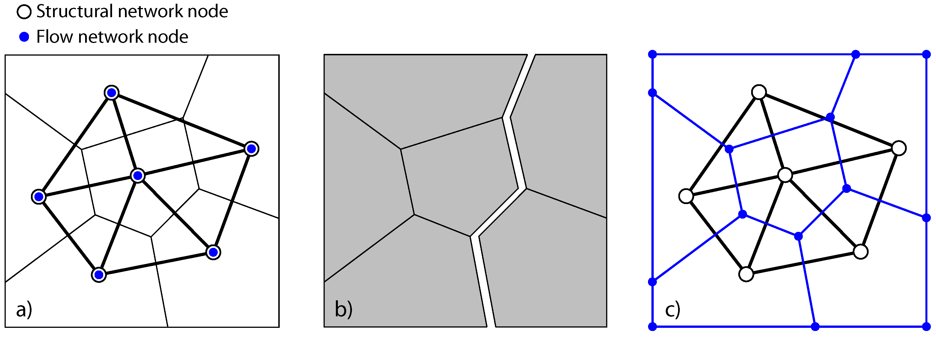
2.1. Discretisation
2.2. Structural Network Model
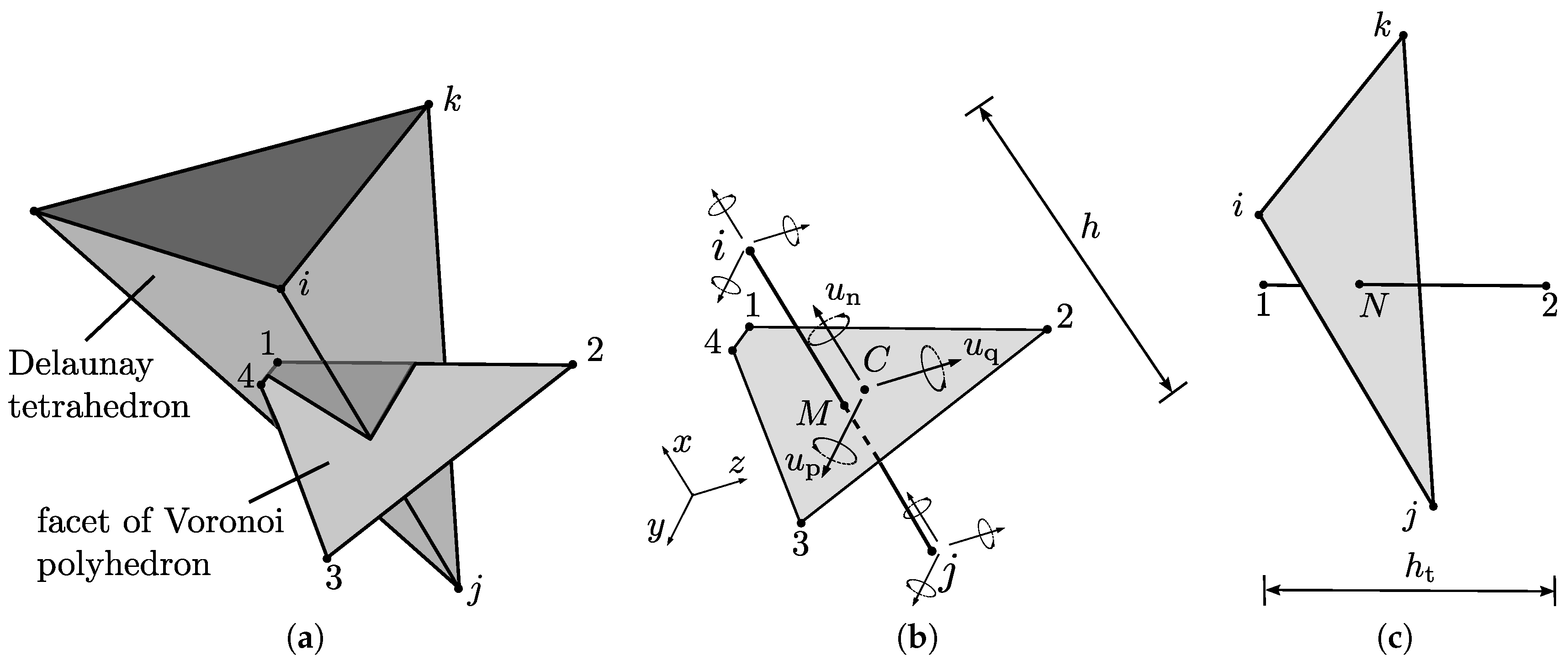
2.2.1. Structural Element
2.2.2. Structural Material
2.3. Transport Model
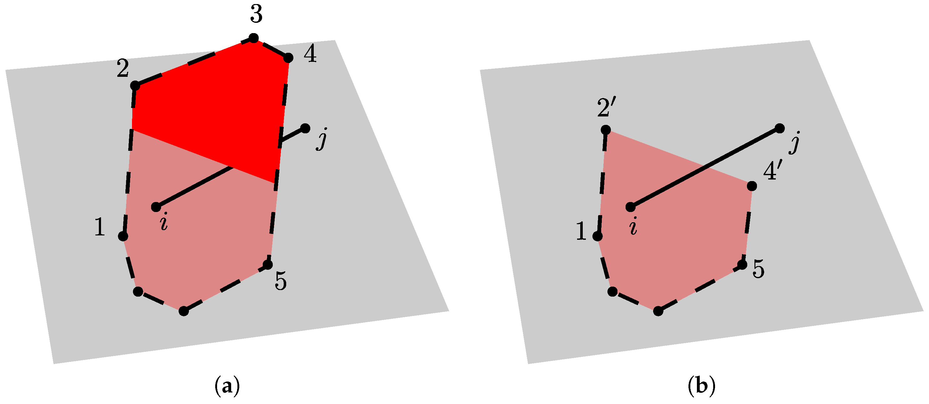
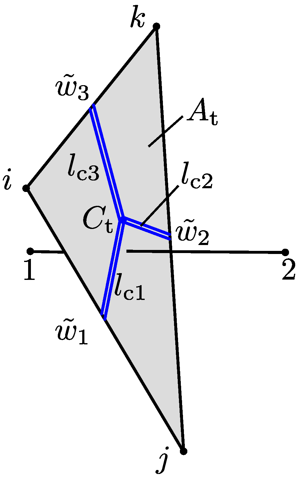
2.3.1. Transport Element
2.3.2. Transport Material
3. Analyses
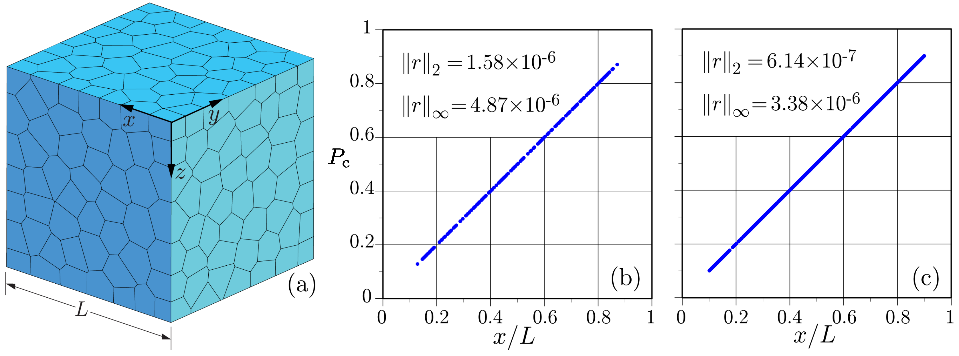
3.1. Steady-State Potential Flow
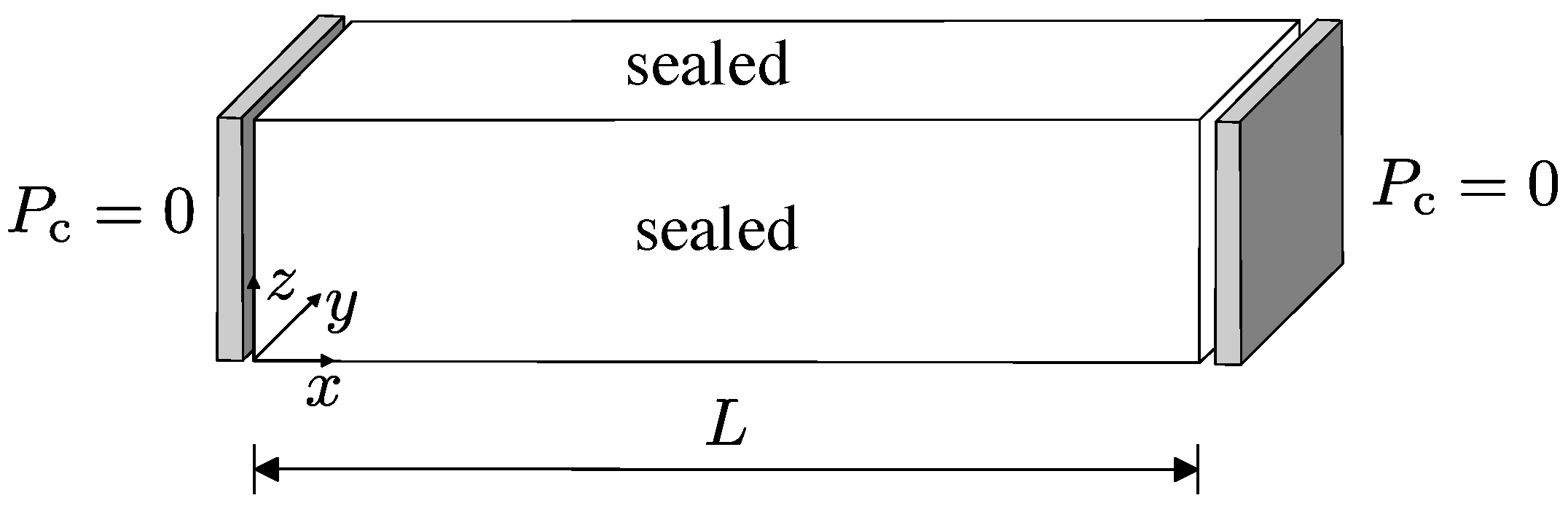
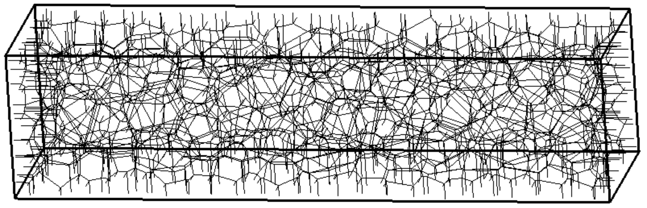
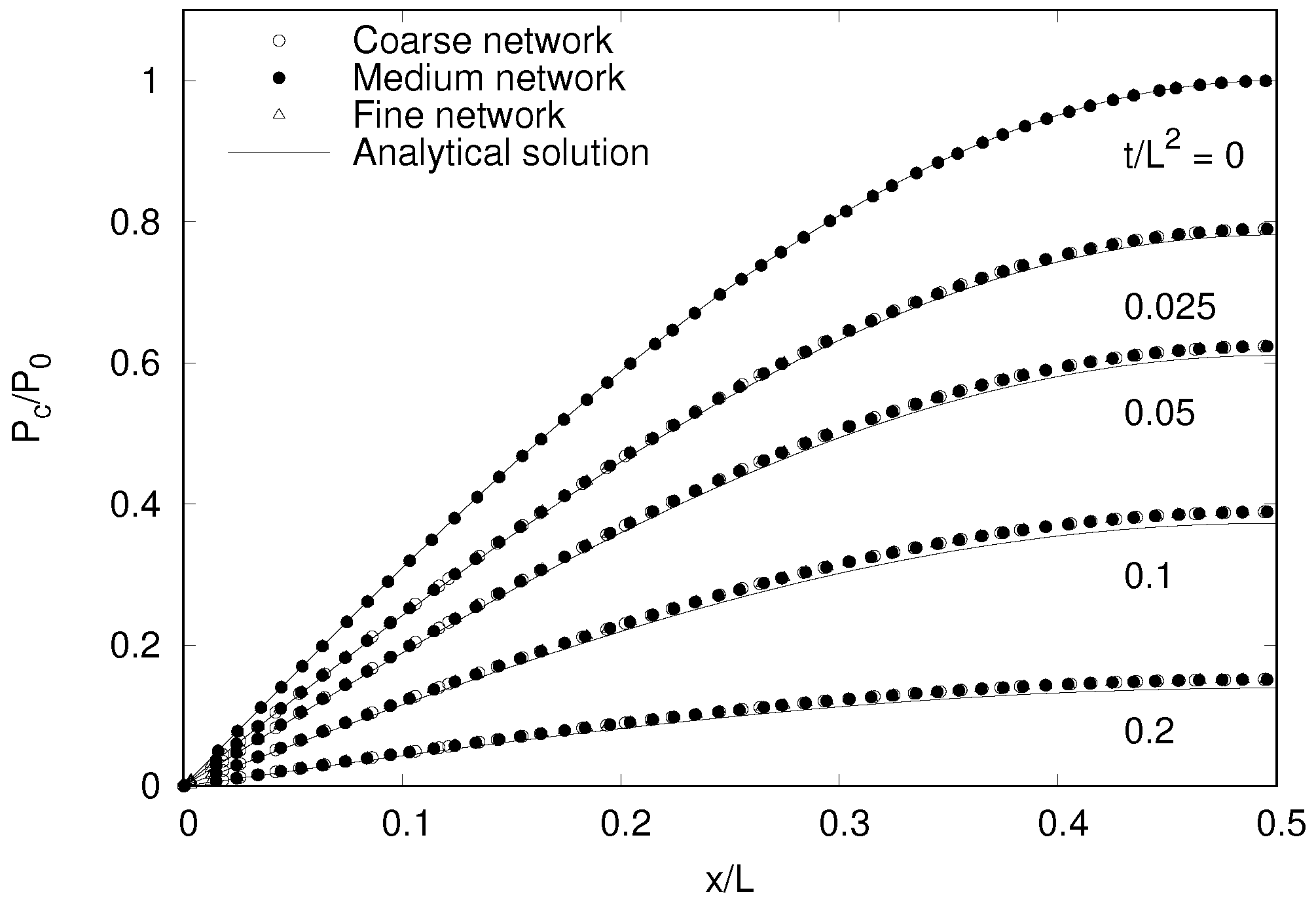
3.2. Nonstationary Transport Analysis
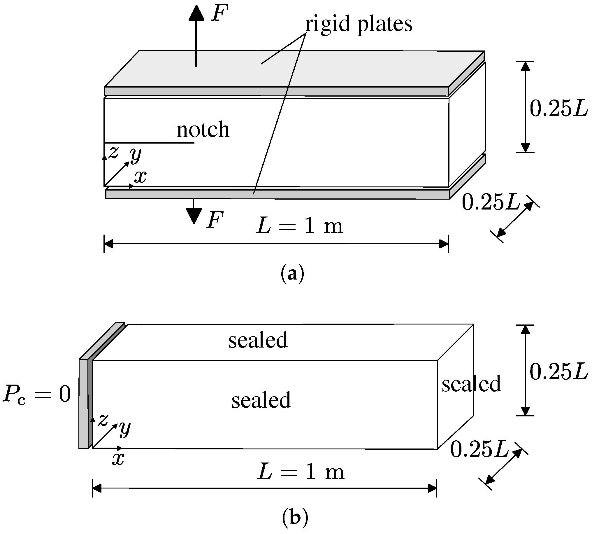
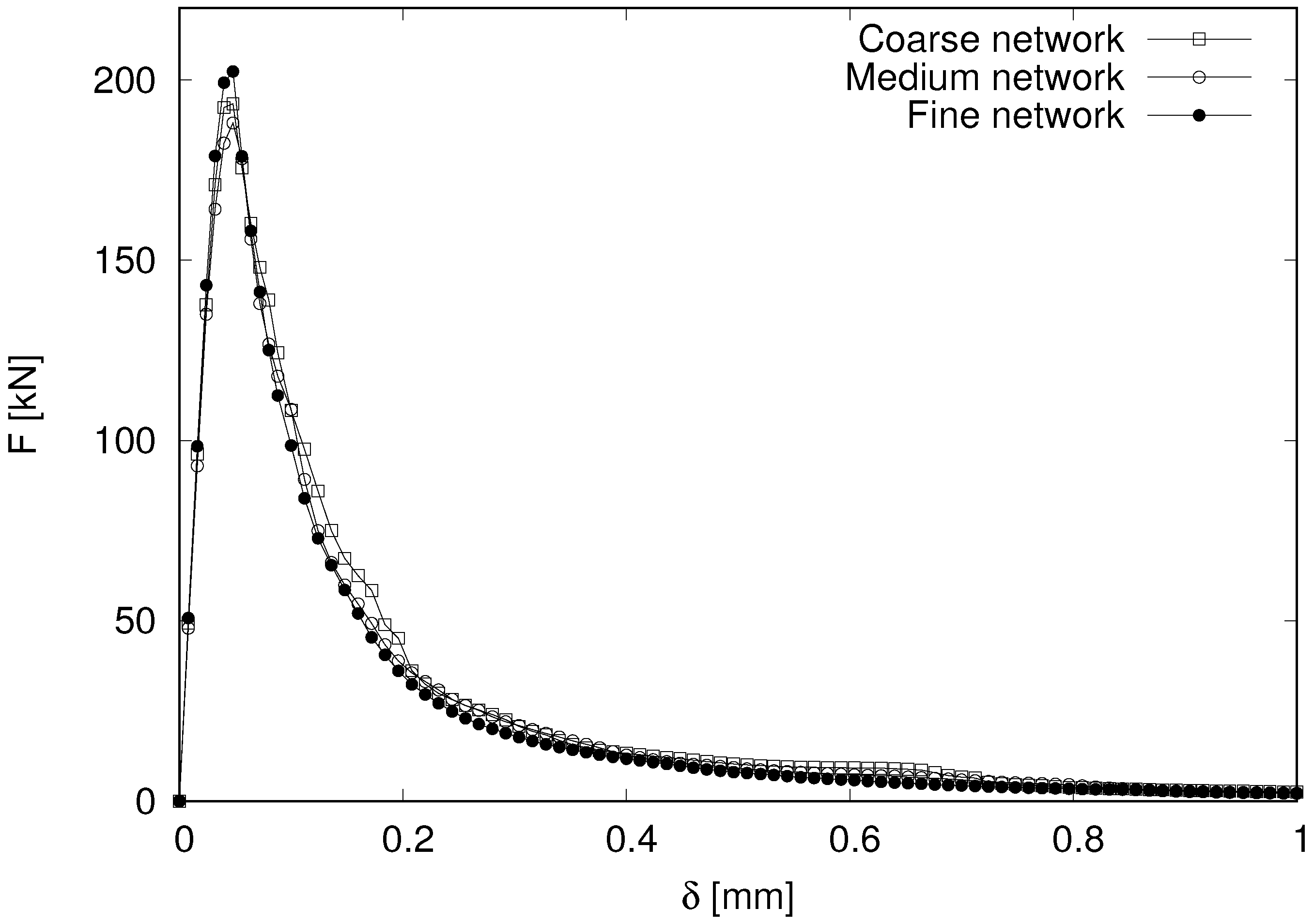
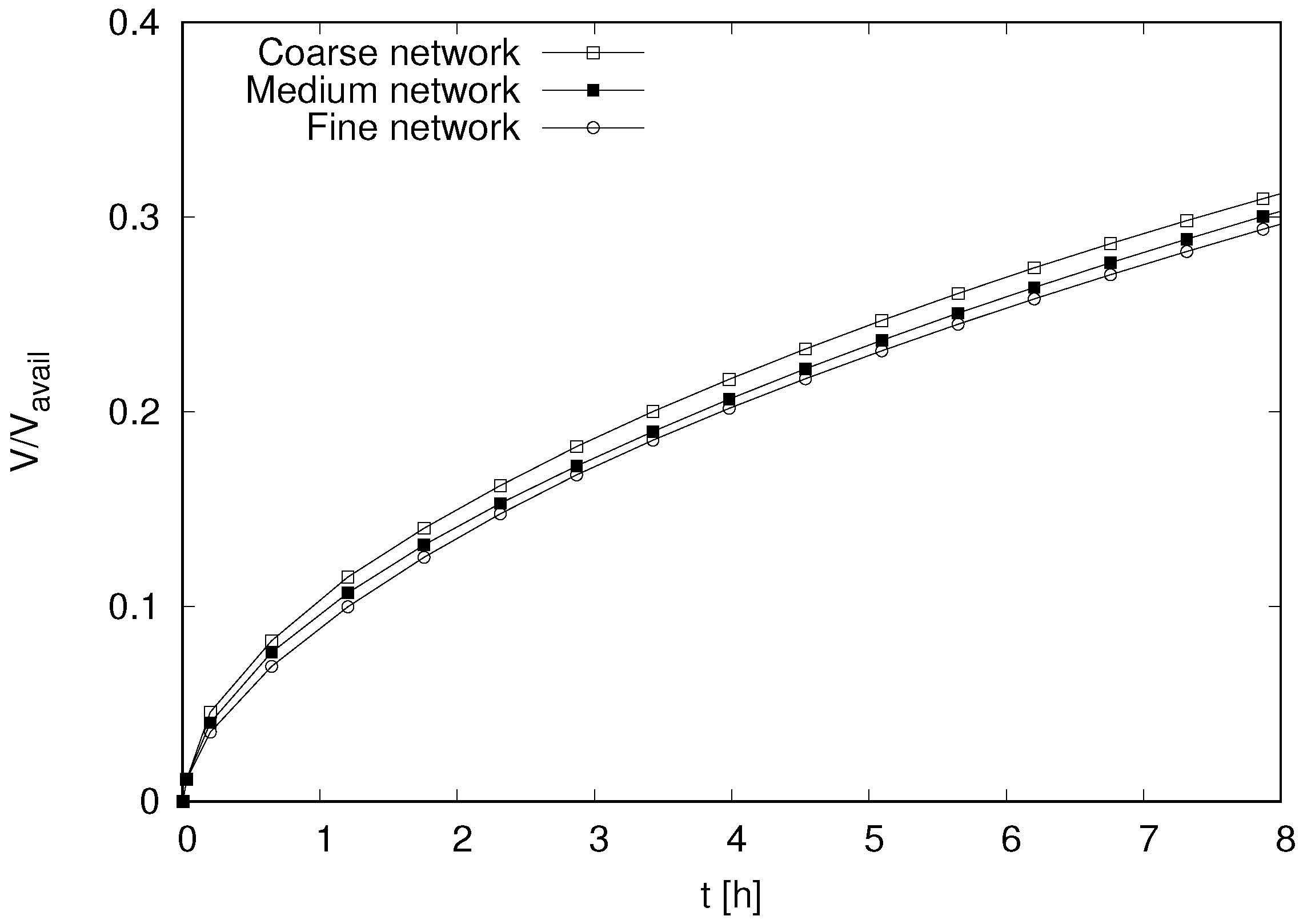
3.3. Coupled Structural-Transport Benchmark
4. Conclusions
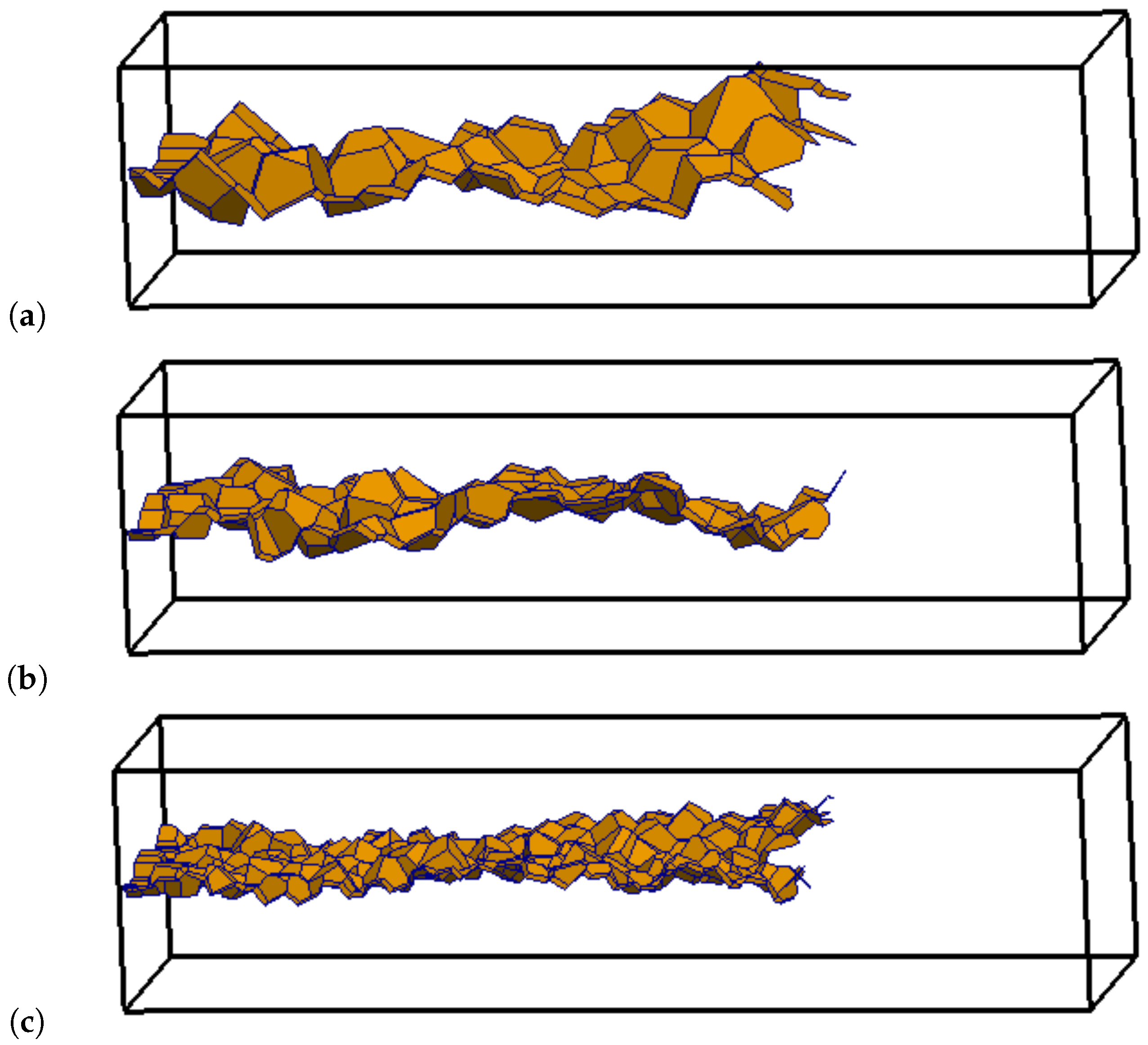
- The network of structural elements, defined by the Delaunay edges, provides element geometry and size independent load-displacement curves, as demonstrated through cohesive fracture simulations of double cantilever beams. The traction free condition is approached without stress locking. Local deviations of the fracture path due to random network generation has very little influence on the load-displacement curves.
- The network of transport elements, defined by the Voronoi edges, provides results for non-stationary transport which are in very good agreement with analytical solutions, and are independent of element geometry and size. The proposed discretisation scheme for the transport network facilitates the enforcement of boundary conditions. Local to a domain boundary, transport elements have one node on the boundary and are directed perpendicular to the boundary.
- The proposed method for coupling the effect of crack opening, determined by the structural network, with transport properties of the transport network yields objective results with respect to element geometry and size. This dual network approach facilitates the simulation of transport along crack paths and from crack faces into the bulk material.
Acknowledgments
Author Contributions
Conflicts of Interest
References
- Roels, S.; Moonen, P.; de Proft, K.; Carmeliet, J. A coupled discrete-continuum approach to simulate moisture effects on damage processes in porous materials. Comput. Methods Appl. Mech. Eng. 2006, 195, 7139–7153. [Google Scholar] [CrossRef]
- Segura, J.M.; Carol, I. Coupled HM analysis using zero-thickness interface elements with double nodes—Part I: Theoretical model. Int. J. Numer. Anal. Methods Geomech. 2008, 32, 2083–2101. [Google Scholar] [CrossRef]
- Segura, J.M.; Carol, I. Coupled HM analysis using zero-thickness interface elements with double nodes—Part II: Verification and application. Int. J. Numer. Anal. Methods Geomech. 2008, 32, 2103–2123. [Google Scholar] [CrossRef]
- Carrier, B.; Granet, S. Numerical modeling of hydraulic fracture problem in permeable medium using cohesive zone model. Eng. Fract. Mech. 2012, 79, 312–328. [Google Scholar] [CrossRef] [Green Version]
- Yao, Y.; Li, L.; Keer, L. Pore pressure cohesive zone modeling of hydraulic fracture in quasi-brittle rocks. Mech. Mater. 2015, 83, 17–29. [Google Scholar] [CrossRef]
- Sadouki, H.; van Mier, J.G.M. Simulation of hygral crack growth in concrete repair system. Mater. Struct. 1997, 203, 518–526. [Google Scholar] [CrossRef]
- Chatzigeorgiou, G.; Picandet, V.; Khelidj, A.; Pijaudier-Cabot, G. Coupling between progressive damage and permeability of concrete: analysis with a discrete model. Int. J. Numer. Anal. Methods Geomech. 2005, 29, 1005–1018. [Google Scholar] [CrossRef]
- Nakamura, H.; Srisoros, W.; Yashiro, R.; Kunieda, M. Time-dependent structural analysis considering mass transfer to evaluate deterioration process of RC structures. J. Adv. Concr. Technol. 2006, 4, 147–158. [Google Scholar] [CrossRef]
- Wang, L.; Soda, M.; Ueda, T. Simulation of chloride diffusivity for cracked concrete based on RBSM and truss network model. J. Adv. Concr. Technol. 2008, 6, 143–155. [Google Scholar] [CrossRef]
- Grassl, P. A lattice approach to model flow in cracked concrete. Cem. Concr. Compos. 2009, 31, 454–460. [Google Scholar] [CrossRef]
- Šavija, B.; Pacheco, J.; Schlangen, E. Lattice modeling of chloride diffusion in sound and cracked concrete. Cem. Concr. Compos. 2013, 42, 30–40. [Google Scholar] [CrossRef]
- Asahina, D.; Houseworth, J.E.; Birkholzer, J.T.; Rutqvist, J.; Bolander, J.E. Hydro-mechanical model for wetting/drying and fracture development in geomaterials. Comput. Geosci. 2014, 65, 13–23. [Google Scholar] [CrossRef]
- Grassl, P.; Fahy, C.; Gallipoli, D.; Wheeler, S.J. On a 2D hydro-mechanical lattice approach for modelling hydraulic fracture. J. Mech. Phys. Solids 2015, 75, 104–118. [Google Scholar] [CrossRef]
- Marina, S.; Derek, I.; Mohamed, P.; Yong, S.; Imo-Imo, E.K. Simulation of the hydraulic fracturing process of fractured rocks by the discrete element method. Environ. Earth Sci. 2015, 73, 8451–8469. [Google Scholar] [CrossRef]
- Damjanac, B.; Detournay, C.; Cundall, P.A. Application of particle and lattice codes to simulation of hydraulic fracturing. Comput. Part. Mech. 2015, 1–13. [Google Scholar] [CrossRef]
- Bolander, J.E.; Saito, S. Fracture analysis using spring networks with random geometry. Eng. Fract. Mech. 1998, 61, 569–591. [Google Scholar] [CrossRef]
- Bolander, J.E.; Sukumar, N. Irregular lattice model for quasistatic crack propagation. Phys. Rev. B 2005, 71, 094106. [Google Scholar] [CrossRef]
- Grassl, P.; Jirásek, M. Meso-scale approach to modelling the fracture process zone of concrete subjected to uniaxial tension. Int. J. Solids Struct. 2010, 47, 957–968. [Google Scholar] [CrossRef]
- Grassl, P.; Davies, T. Lattice modelling of corrosion induced cracking and bond in reinforced concrete. Cem. Concr. Compos. 2011, 33, 918–924. [Google Scholar] [CrossRef]
- Bolander, J.E.; Berton, S. Simulation of shrinkage induced cracking in cement composite overlays. Cem. Concr. Compos. 2004, 26, 861–871. [Google Scholar] [CrossRef]
- Saka, T. Simulation of Reinforced Concrete Durability: Dual-Lattice Models of Crack-Assisted Mass Transport. Ph.D. Thesis, University of California, Davis, CA, USA, 2012. [Google Scholar]
- Okabe, A.; Boots, B.; Sugihara, K.; Chiu, S.N. Spatial Tessellations: Concepts and Applications of Voronoi Diagrams; Wiley: New York, NY, USA, 2000. [Google Scholar]
- Yip, M.; Mohle, J.; Bolander, J.E. Automated modeling of three-dimensional structural components using irregular lattices. Comput. Aided Civ. Infrastruct. Eng. 2005, 20, 393–407. [Google Scholar] [CrossRef]
- Strang, G. Introduction to Applied Mathematics; Wellesley-Cambridge Press: Wellesley, MA, USA, 1986. [Google Scholar]
- Kawai, T. New discrete models and their application to seismic response analysis of structures. Nucl. Eng. Des. 1978, 48, 207–229. [Google Scholar] [CrossRef]
- Berton, S.; Bolander, J.E. Crack band model of fracture in irregular lattices. Comput. Methods Appl. Mech. Eng. 2006, 195, 7172–7181. [Google Scholar] [CrossRef]
- Mazars, J.; Pijaudier-Cabot, G. Continuum damage theory—Application to concrete. J. Eng. Mech. 1989, 115, 345–365. [Google Scholar] [CrossRef]
- Lemaitre, J.; Chaboche, J.L. Mechanics of Solid Materials; Cambridge University Press: Cambridge, UK, 1990. [Google Scholar]
- Maekawa, K.; Ishida, T.; Kishi, T. Multi-Scale Modeling of Structural Concrete; CRC Press: Boca Raton, FL, USA, 2008. [Google Scholar]
- Lewis, R.W.; Morgan, K.; Thomas, H.R.; Seetharamu, K. The Finite Element Method in Heat Transfer Analysis; John Wiley & Sons: Hoboken, NJ, USA, 1996. [Google Scholar]
- van Genuchten, M.T. A closed-form equation for predicting the hydraulic conductivity of unsaturated soils. Soil Sci. Soc. Am. 1980, 44, 892–898. [Google Scholar] [CrossRef]
- Baroghel-Bouny, V.; Mainguy, M.; Lassabatere, T.; Coussy, O. Characterization and identification of equilibrium and transfer moisture properties for ordinary and high-performance cementitious materials. Cem. Concr. Res. 1999, 29, 1225–1238. [Google Scholar] [CrossRef]
- Akhavan, A.; Shafaatian, S.M.H.; Rajabipour, F. Quantifying the effects of crack width, tortuosity, and roughness on water permeability of cracked mortars. Cem. Concr. Res. 2012, 42, 313–320. [Google Scholar] [CrossRef]
- Witherspoon, P.A.; Wang, J.S.Y.; Iawai, K.; Gale, J.E. Validity of cubic law for fluid flow in a deformable rock fracture. Water Resour. Res. 1980, 16, 1016–1024. [Google Scholar] [CrossRef]
- Asahina, D.; Landis, E.N.; Bolander, J.E. Modeling of phase interfaces during pre-critical crack growth in concrete. Cem. Concr. Compos. 2011, 33, 966–977. [Google Scholar] [CrossRef]
- Patzák, B. OOFEM—An object-oriented simulation tool for advanced modeling of materials and structures. Acta Polytech. 2012, 52, 59–66. [Google Scholar]


| Symbol | (Units) | Definition |
|---|---|---|
| (m) | cross-sectional area of the tetrahedron face | |
| a | (Pa) | parameter in van Genuchten model |
| , | matrices expressing rigid body kinematics | |
| c | (s/m) | capacity of the material |
| (m s) | element capacity matrix | |
| C | (m) | centroid of mid-cross-section |
| ratio of compressive and tensile strength | ||
| (Pa) | material stiffness matrix | |
| (m) | minimum distance between nodes | |
| , | (m) | eccentricities between the midpoint of the network element and the centroid C |
| E | (Pa) | Young’s modulus |
| (N) | acting structural forces | |
| loading function | ||
| (Pa) | tensile strength | |
| (Pa) | shear strength | |
| (Pa) | compressive strength | |
| f | (kg/m) | outward flux normal to the boundary |
| (J/m) | fracture energy | |
| h | (m) | length of structural element |
| (m) | length of transport element | |
| unity matrix | ||
| (m) | polar moment of area | |
| and | (m) | two principal second moments of area of the cross-section |
| element stiffness matrix | ||
| rotational stiffness at point C | ||
| (m) | crack length | |
| L | (m) | length of specimen |
| m | parameter in van Genuchten model | |
| n, p, q | (m) | coordinates of mid-cross-sections |
| (Pa) | capillary suction (tension positive) | |
| (Pa) | pressure in the wetting fluid | |
| (Pa) | pressure in the non-wetting fluid | |
| ratio of shear and tensile strength | ||
| S | degree of saturation | |
| t | (s) | time |
| , , | (m) | displacement discontinuities |
| , , | (m) | translational degrees of freedom |
| vector of degrees of freedom of structural element | ||
| (m) | vector of translational part of degrees of freedom | |
| vector of rotational part of degrees of freedom | ||
| (m) | vector of displacement discontinuities | |
| V | (m) | volume |
| (m) | available volume to be filled | |
| (m) | total volume of the specimen | |
| , and | (m) | crack opening components |
| (m) | displacement threshold which determines the initial slope of the softening curve | |
| (m) | equivalent crack opening | |
| x, y, z | (m) | Cartesian coordinates |
| (s) | initial conductivity of the undamaged material | |
| (s) | change of the conductivity due to fracture | |
| α | (s) | conductivity |
| conductivity matrix | ||
| γ | input parameter, which controls Poisson’s ratio of the structural network | |
| , | boundary segments | |
| δ | (m) | load-point-displacement |
| ε | strain vector | |
| , , | strain components | |
| strain threshold | ||
| θ | (kg/m) | moisture content |
| (kg/m) | residual moisture content | |
| (kg/m) | saturated moisture content | |
| κ | (m) | intrinsic permeability |
| history variable in damage model | ||
| relative permeability | ||
| μ | (Pa s) | dynamic (absolute) viscosity |
| ξ | tortuosity factor | |
| ρ | (kg/m) | density of the fluid |
| (Pa) | continuum stress | |
| σ | (Pa) | stress vector |
| , , | (Pa) | stress components |
| , , | rotational degrees of freedom | |
| ω | damage variable | |
| ∇ | divergence operator |
| Network Type | Node Definition | Element Definition | Nodal Count * | Element Count * |
|---|---|---|---|---|
| Conventional | Delaunay vertex | Delaunay edge | 330 | 1800 |
| Proposed | Voronoi vertex | Voronoi edge | 2880 | 5440 |
© 2016 by the authors; licensee MDPI, Basel, Switzerland. This article is an open access article distributed under the terms and conditions of the Creative Commons Attribution (CC-BY) license (http://creativecommons.org/licenses/by/4.0/).
Share and Cite
Grassl, P.; Bolander, J. Three-Dimensional Network Model for Coupling of Fracture and Mass Transport in Quasi-Brittle Geomaterials. Materials 2016, 9, 782. https://doi.org/10.3390/ma9090782
Grassl P, Bolander J. Three-Dimensional Network Model for Coupling of Fracture and Mass Transport in Quasi-Brittle Geomaterials. Materials. 2016; 9(9):782. https://doi.org/10.3390/ma9090782
Chicago/Turabian StyleGrassl, Peter, and John Bolander. 2016. "Three-Dimensional Network Model for Coupling of Fracture and Mass Transport in Quasi-Brittle Geomaterials" Materials 9, no. 9: 782. https://doi.org/10.3390/ma9090782