
The Potential of Multi-Task Learning in CFDST Design: Load-Bearing Capacity Design with Three MTL Models

Abstract
:1. Introduction
2. Materials and Methods
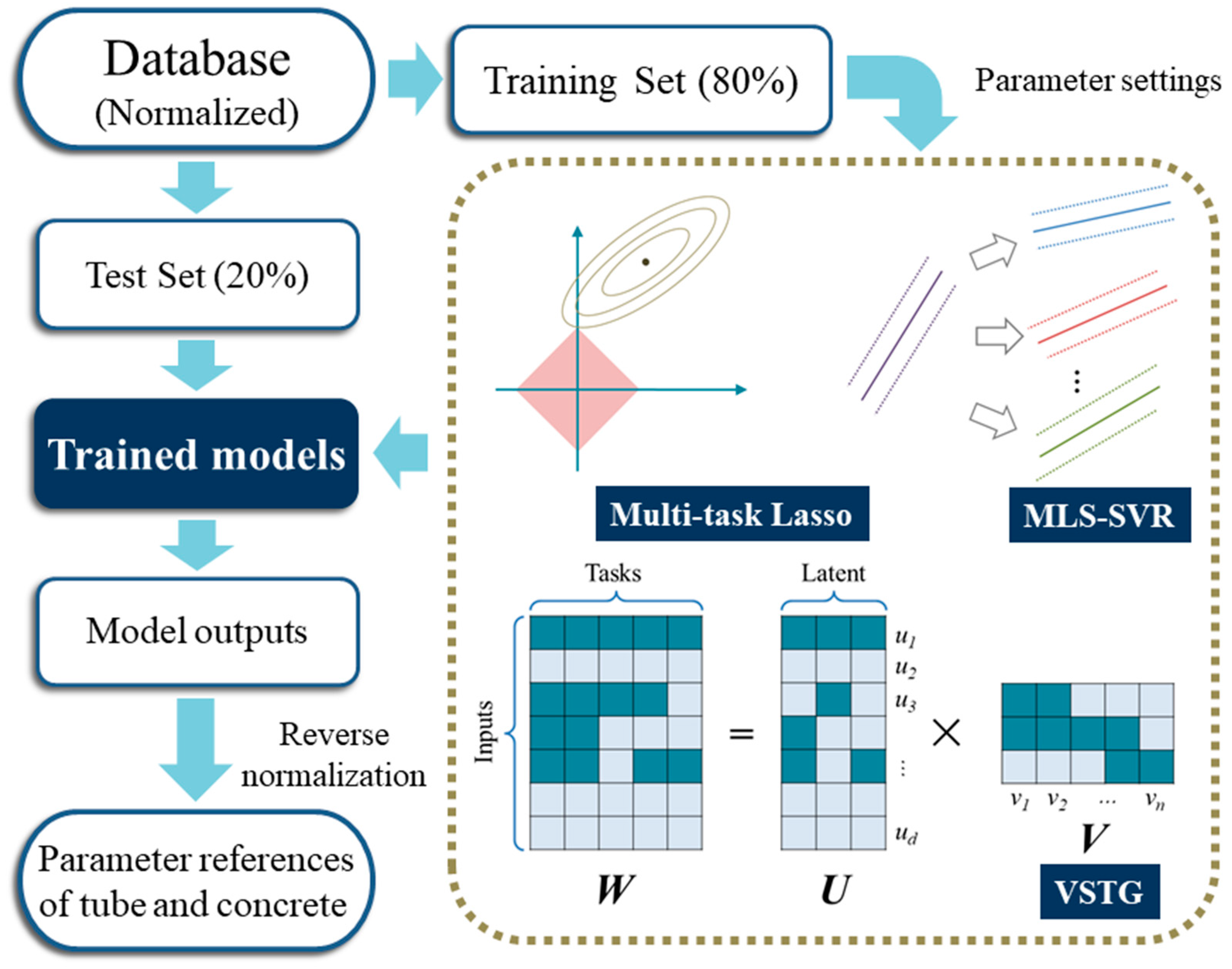
2.1. Multi-Task Learning Models
2.1.1. Multi-Task Lasso
2.1.2. VSTG
2.1.3. MLS-SVR
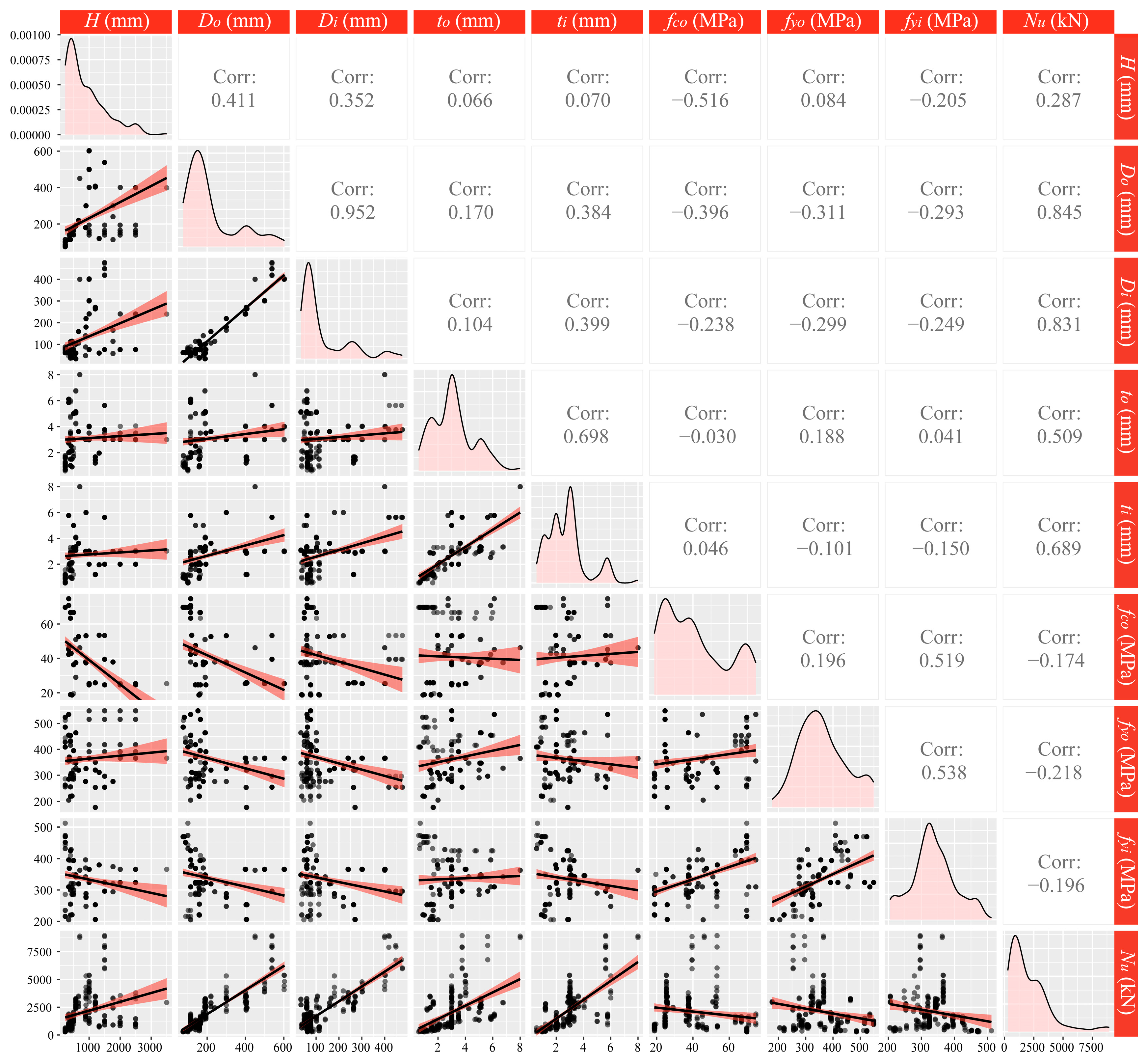
2.2. Database
2.3. Model Development
3. Results
4. Discussion
4.1. Nonlinearity
- Cause A: The provided input features did not contain the key information related to the strength tasks. For task fyi and fco, all input features were useless.
- Cause B: There was a certain non-linear relationship between input features and strength tasks. Thereby, linear models were unable to simulate this nonlinearity well.
4.2. Model Interpretability
- Group 1 (task Di): The coefficient of the second base M2 is significantly higher than the other two;
- Group 2 (task ti): The coefficient of the second base M2 is significantly lower than the other two;
- Group 3 (task fyi and fco): The first base is obviously important, while the values of the other two are almost 0.
4.3. Limitations and Future Work
- The samples collected in the database were all CFDSTs with circular cross-sections, as this shape is the most conventional. CFDSTs of other shapes may have more parameters, so their design must be more complex.
- MTL is a data-driven approach, and the performance of this technique depends on the quantity and quality of data. Currently, the uniaxial compression cases of CFDSTs are sufficient, while cases of other property trials are still lacking.
- The interpretability of linear models can reveal the potential connection among CFDST parameters. However, this connection is purely mathematical, and the mechanism behind it still remains a mystery.
5. Conclusions
- With 227 uniaxial compression cases of CFDSTs collected from previous literature, three kinds of MTL models were trained to provide multiple parameters for CFDST design. Based on a specific application scenario, the development process of the MTL models was demonstrated.
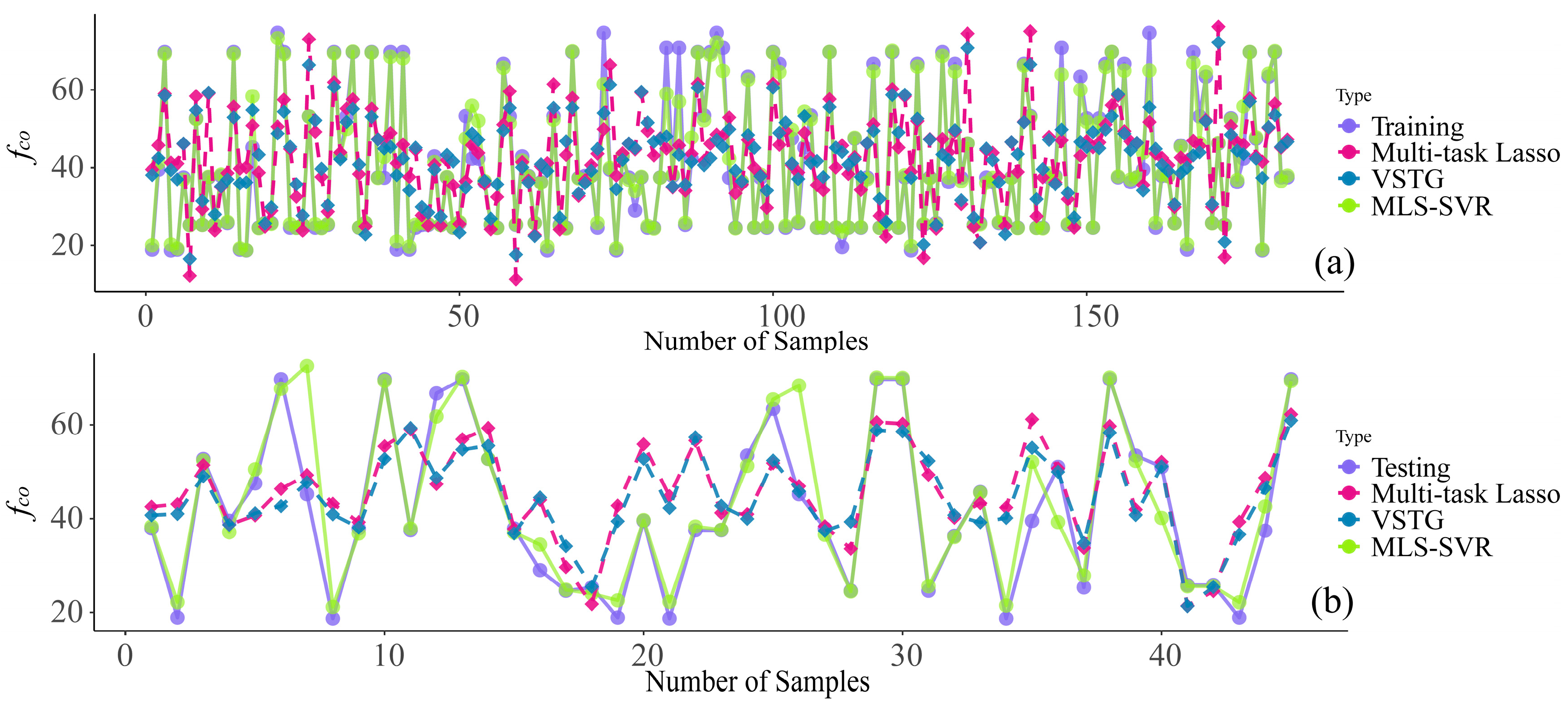
- During the testing phase, MLS-SVR was able to accurately provide reliable CFDST parameters, while the other two linear models, multi-task Lasso and VSTG, were unable to provide valuable parameters of inner steel tube strength and concrete strength.
- The distribution of scattered points reflected the potential nonlinearity in the task fyi and fco, and the connotation in scatter distribution was discussed in detail. Furthermore, the coefficient matrices of two linear models and the potential group structure among the CFDST parameters were clarified.
- At the end of Section 4, the limitations of the study and future work are also summarized.
Author Contributions
Funding
Institutional Review Board Statement
Informed Consent Statement
Data Availability Statement
Conflicts of Interest
Appendix A

| Outputs | Dataset | R2 | RMSE | RRMSE | ρ |
|---|---|---|---|---|---|
| Di | Trn_experiment_1 | 0.925798241 | 30.54154609 | 0.240264793 | 0.12244763 |
| Trn_experiment_2 | 0.925798326 | 30.54154601 | 0.240265398 | 0.122447936 | |
| Trn_experiment_3 | 0.925798412 | 30.54154593 | 0.240266004 | 0.122448242 | |
| Trn_experiment_4 | 0.925798497 | 30.54154587 | 0.24026661 | 0.122448548 | |
| Trn_experiment_5 | 0.921823761 | 31.23514035 | 0.24540618 | 0.125199791 | |
| Trn_mean | 0.925003447 | 30.68026485 | 0.241293797 | 0.122998429 | |
| Tst_experiment_1 | 0.903852591 | 34.90496 | 0.274591 | 0.140764 | |
| Tst_experiment_2 | 0.903852949 | 34.90481 | 0.27459 | 0.140764 | |
| Tst_experiment_3 | 0.903853308 | 34.90466 | 0.27459 | 0.140764 | |
| Tst_experiment_4 | 0.903853667 | 34.90451 | 0.27459 | 0.140764 | |
| Tst_experiment_5 | 0.898420822 | 35.83429 | 0.28154 | 0.144539 | |
| Tst_mean | 0.902766668 | 35.09065 | 0.27598 | 0.141519 | |
| ti | Trn_experiment_1 | 0.647650602 | 0.865708461 | 0.312352516 | 0.173070786 |
| Trn_experiment_2 | 0.647650541 | 0.86570846 | 0.312353227 | 0.173071183 | |
| Trn_experiment_3 | 0.647650481 | 0.865708459 | 0.312353938 | 0.173071581 | |
| Trn_experiment_4 | 0.64765042 | 0.865708458 | 0.312354649 | 0.173071978 | |
| Trn_experiment_5 | 0.642129795 | 0.87523493 | 0.30854615 | 0.171287964 | |
| Trn_mean | 0.646546368 | 0.867613754 | 0.311592096 | 0.172714698 | |
| Tst_experiment_1 | 0.895809286 | 0.497392 | 0.179462 | 0.092198 | |
| Tst_experiment_2 | 0.895808763 | 0.497392 | 0.179462 | 0.092199 | |
| Tst_experiment_3 | 0.89580824 | 0.497392 | 0.179463 | 0.092199 | |
| Tst_experiment_4 | 0.895807718 | 0.497392 | 0.179463 | 0.092199 | |
| Tst_experiment_5 | 0.896319131 | 0.522132 | 0.184067 | 0.094551 | |
| Tst_mean | 0.895910627 | 0.50234 | 0.180383 | 0.092669 | |
| fyi | Trn_experiment_1 | 0.257824781 | 56.61053299 | 0.166176103 | 0.110213567 |
| Trn_experiment_2 | 0.257826623 | 56.61053286 | 0.166176058 | 0.110213404 | |
| Trn_experiment_3 | 0.257828465 | 56.61053274 | 0.166176012 | 0.110213242 | |
| Trn_experiment_4 | 0.257830307 | 56.61053264 | 0.166175967 | 0.110213079 | |
| Trn_experiment_5 | 0.143605727 | 61.05929462 | 0.175032617 | 0.12693149 | |
| Trn_mean | 0.234983181 | 57.50028517 | 0.167947351 | 0.113556956 | |
| Tst_experiment_1 | 0.457067241 | 49.81142 | 0.146218 | 0.087239 | |
| Tst_experiment_2 | 0.457071203 | 49.81112 | 0.146217 | 0.087238 | |
| Tst_experiment_3 | 0.457075164 | 49.81082 | 0.146216 | 0.087237 | |
| Tst_experiment_4 | 0.457079126 | 49.81052 | 0.146215 | 0.087237 | |
| Tst_experiment_5 | 0.309128976 | 56.65101 | 0.162396 | 0.104368 | |
| Tst_mean | 0.427484342 | 51.17898 | 0.149452 | 0.090664 | |
| fco | Trn_experiment_1 | 0.382329222 | 13.91468957 | 0.305536581 | 0.188797713 |
| Trn_experiment_2 | 0.382332284 | 13.91468953 | 0.305535146 | 0.188796538 | |
| Trn_experiment_3 | 0.382335346 | 13.91468949 | 0.305533712 | 0.188795363 | |
| Trn_experiment_4 | 0.382338409 | 13.91468947 | 0.305532277 | 0.188794187 | |
| Trn_experiment_5 | 0.349522654 | 14.25304033 | 0.319577939 | 0.20084028 | |
| Trn_mean | 0.375771583 | 13.98235968 | 0.308343131 | 0.191204816 | |
| Tst_experiment_1 | 0.388893448 | 13.62725 | 0.299225 | 0.184296 | |
| Tst_experiment_2 | 0.388897421 | 13.62727 | 0.299224 | 0.184295 | |
| Tst_experiment_3 | 0.388901394 | 13.62728 | 0.299223 | 0.184294 | |
| Tst_experiment_4 | 0.388905367 | 13.62729 | 0.299222 | 0.184293 | |
| Tst_experiment_5 | 0.383469564 | 13.54646 | 0.303735 | 0.187578 | |
| Tst_mean | 0.387813439 | 13.61111 | 0.300126 | 0.184951 |
| Outputs | Dataset | R2 | RMSE | RRMSE | ρ |
|---|---|---|---|---|---|
| Di | Trn_experiment_1 | 0.922420 | 31.20567 | 0.244677 | 0.124808 |
| Trn_experiment_2 | 0.921584 | 31.29855 | 0.245879 | 0.125449 | |
| Trn_experiment_3 | 0.921693 | 31.27291 | 0.245672 | 0.12534 | |
| Trn_experiment_4 | 0.921771 | 31.25197 | 0.245519 | 0.125259 | |
| Trn_experiment_5 | 0.921824 | 31.23514 | 0.245406 | 0.125200 | |
| Trn_mean | 0.921858 | 31.25285 | 0.245431 | 0.125211 | |
| Tst_experiment_1 | 0.899683 | 35.70926 | 0.279989 | 0.143693 | |
| Tst_experiment_2 | 0.898060 | 35.89606 | 0.281997 | 0.144788 | |
| Tst_experiment_3 | 0.898216 | 35.87198 | 0.281801 | 0.144681 | |
| Tst_experiment_4 | 0.898334 | 35.85119 | 0.281651 | 0.144599 | |
| Tst_experiment_5 | 0.898421 | 35.83429 | 0.28154 | 0.144539 | |
| Tst_mean | 0.898543 | 35.83256 | 0.281396 | 0.14446 | |
| ti | Trn_experiment_1 | 0.64555 | 0.870096 | 0.308432 | 0.171022 |
| Trn_experiment_2 | 0.642602 | 0.874941 | 0.308653 | 0.171319 | |
| Trn_experiment_3 | 0.642569 | 0.874921 | 0.308611 | 0.171298 | |
| Trn_experiment_4 | 0.642411 | 0.875007 | 0.308572 | 0.171286 | |
| Trn_experiment_5 | 0.642130 | 0.875235 | 0.308546 | 0.171288 | |
| Trn_mean | 0.643052 | 0.874040 | 0.308563 | 0.171243 | |
| Tst_experiment_1 | 0.897740 | 0.513348 | 0.181972 | 0.093439 | |
| Tst_experiment_2 | 0.897543 | 0.518708 | 0.182985 | 0.093964 | |
| Tst_experiment_3 | 0.897429 | 0.51924 | 0.183152 | 0.094053 | |
| Tst_experiment_4 | 0.896939 | 0.520482 | 0.183548 | 0.094269 | |
| Tst_experiment_5 | 0.896319 | 0.522132 | 0.184067 | 0.094551 | |
| Tst_mean | 0.897194 | 0.518782 | 0.183145 | 0.094055 | |
| fyi | Trn_experiment_1 | 0.136017 | 61.32048 | 0.175747 | 0.128395 |
| Trn_experiment_2 | 0.142423 | 61.08823 | 0.175156 | 0.127165 | |
| Trn_experiment_3 | 0.142487 | 61.08705 | 0.175144 | 0.127149 | |
| Trn_experiment_4 | 0.142957 | 61.07670 | 0.175097 | 0.127057 | |
| Trn_experiment_5 | 0.143606 | 61.05929 | 0.175033 | 0.126931 | |
| Trn_mean | 0.141498 | 61.12635 | 0.175235 | 0.127339 | |
| Tst_experiment_1 | 0.295738 | 56.90902 | 0.163104 | 0.10565 | |
| Tst_experiment_2 | 0.305408 | 56.78643 | 0.162821 | 0.104868 | |
| Tst_experiment_3 | 0.306126 | 56.75469 | 0.162723 | 0.104760 | |
| Tst_experiment_4 | 0.307393 | 56.71041 | 0.162579 | 0.104591 | |
| Tst_experiment_5 | 0.309129 | 56.65101 | 0.162396 | 0.104368 | |
| Tst_mean | 0.304759 | 56.76231 | 0.162725 | 0.104847 | |
| fco | Trn_experiment_1 | 0.355196 | 14.18623 | 0.317429 | 0.198892 |
| Trn_experiment_2 | 0.349209 | 14.26040 | 0.319686 | 0.200941 | |
| Trn_experiment_3 | 0.349363 | 14.25735 | 0.319629 | 0.200889 | |
| Trn_experiment_4 | 0.349489 | 14.25495 | 0.319587 | 0.200850 | |
| Trn_experiment_5 | 0.349523 | 14.25304 | 0.319578 | 0.200840 | |
| Trn_mean | 0.350556 | 14.24239 | 0.319182 | 0.200483 | |
| Tst_experiment_1 | 0.389745 | 13.47301 | 0.301470 | 0.185600 | |
| Tst_experiment_2 | 0.383357 | 13.55413 | 0.303853 | 0.187661 | |
| Tst_experiment_3 | 0.383610 | 13.54961 | 0.303762 | 0.187581 | |
| Tst_experiment_4 | 0.383550 | 13.54818 | 0.303742 | 0.187574 | |
| Tst_experiment_5 | 0.383470 | 13.54646 | 0.303735 | 0.187578 | |
| Tst_mean | 0.384746 | 13.53428 | 0.303312 | 0.187199 |
| Outputs | Dataset | R2 | RMSE | RRMSE | ρ |
|---|---|---|---|---|---|
| Di | Trn_experiment_1 | 0.997956 | 4.950633 | 0.04127 | 0.020645 |
| Trn_experiment_2 | 0.998098 | 4.774466 | 0.039817 | 0.019918 | |
| Trn_experiment_3 | 0.99828 | 4.541585 | 0.037884 | 0.01895 | |
| Trn_experiment_4 | 0.99679 | 6.21027 | 0.051617 | 0.025829 | |
| Trn_experiment_5 | 0.997152 | 5.847266 | 0.04864 | 0.024337 | |
| Trn_mean | 0.997655 | 5.264844 | 0.043846 | 0.021936 | |
| Tst_experiment_1 | 0.966752 | 20.16726 | 0.168119 | 0.08477 | |
| Tst_experiment_2 | 0.967065 | 20.06718 | 0.167353 | 0.084377 | |
| Tst_experiment_3 | 0.96684 | 20.11983 | 0.16783 | 0.084623 | |
| Tst_experiment_4 | 0.965648 | 20.61851 | 0.171372 | 0.086435 | |
| Tst_experiment_5 | 0.966064 | 20.46098 | 0.170203 | 0.085836 | |
| Tst_mean | 0.966474 | 20.28675 | 0.168976 | 0.085208 | |
| ti | Trn_experiment_1 | 0.977555 | 0.221349 | 0.086169 | 0.043329 |
| Trn_experiment_2 | 0.977566 | 0.221087 | 0.086098 | 0.043293 | |
| Trn_experiment_3 | 0.980432 | 0.206541 | 0.080415 | 0.040406 | |
| Trn_experiment_4 | 0.963974 | 0.280518 | 0.109174 | 0.055088 | |
| Trn_experiment_5 | 0.967474 | 0.266504 | 0.103741 | 0.0523 | |
| Trn_mean | 0.9734 | 0.2392 | 0.093119 | 0.046883 | |
| Tst_experiment_1 | 0.901291 | 0.402229 | 0.156584 | 0.080326 | |
| Tst_experiment_2 | 0.901474 | 0.401589 | 0.156391 | 0.080223 | |
| Tst_experiment_3 | 0.898315 | 0.408791 | 0.159159 | 0.081712 | |
| Tst_experiment_4 | 0.916494 | 0.368955 | 0.143593 | 0.073361 | |
| Tst_experiment_5 | 0.912926 | 0.376779 | 0.146668 | 0.075004 | |
| Tst_mean | 0.9061 | 0.391669 | 0.152479 | 0.078125 | |
| fyi | Trn_experiment_1 | 0.989376 | 6.803098 | 0.019868 | 0.009961 |
| Trn_experiment_2 | 0.989653 | 6.711025 | 0.019602 | 0.009826 | |
| Trn_experiment_3 | 0.99114 | 6.20726 | 0.018126 | 0.009083 | |
| Trn_experiment_4 | 0.980407 | 9.245705 | 0.027043 | 0.013588 | |
| Trn_experiment_5 | 0.982968 | 8.620965 | 0.025204 | 0.012656 | |
| Trn_mean | 0.986709 | 7.517611 | 0.021969 | 0.011023 | |
| Tst_experiment_1 | 0.965078 | 12.61071 | 0.036829 | 0.018578 | |
| Tst_experiment_2 | 0.965056 | 12.62965 | 0.036889 | 0.018608 | |
| Tst_experiment_3 | 0.965206 | 12.59698 | 0.036785 | 0.018555 | |
| Tst_experiment_4 | 0.964875 | 12.67916 | 0.037085 | 0.018708 | |
| Tst_experiment_5 | 0.964985 | 12.64765 | 0.036977 | 0.018653 | |
| Tst_mean | 0.96504 | 12.63283 | 0.036913 | 0.018621 | |
| fco | Trn_experiment_1 | 0.977615 | 2.637616 | 0.060853 | 0.030599 |
| Trn_experiment_2 | 0.978519 | 2.583422 | 0.059613 | 0.029968 | |
| Trn_experiment_3 | 0.980582 | 2.456158 | 0.056692 | 0.028485 | |
| Trn_experiment_4 | 0.969402 | 3.094903 | 0.071324 | 0.035939 | |
| Trn_experiment_5 | 0.97116 | 3.000334 | 0.069161 | 0.034833 | |
| Trn_mean | 0.975456 | 2.754487 | 0.063529 | 0.031965 | |
| Tst_experiment_1 | 0.865928 | 6.502839 | 0.15003 | 0.077713 | |
| Tst_experiment_2 | 0.865614 | 6.515199 | 0.15034 | 0.077881 | |
| Tst_experiment_3 | 0.86555 | 6.522601 | 0.150551 | 0.077992 | |
| Tst_experiment_4 | 0.865382 | 6.473133 | 0.149178 | 0.077284 | |
| Tst_experiment_5 | 0.865663 | 6.478995 | 0.149347 | 0.077365 | |
| Tst_mean | 0.865628 | 6.498553 | 0.149889 | 0.077647 |
References
- Chrysanidis, T.; Tegos, I. Axial and transverse strengthening of R/C circular columns: Conventional and new type of steel and hybrid jackets using high-strength mortar. J. Build. Eng. 2020, 30, 23. [Google Scholar] [CrossRef]
- Fan, J.-H.; Wang, W.-D.; Shi, Y.-L.; Ji, S.-H. Torsional behaviour of tapered CFDST members with large void ratio. J. Build. Eng. 2022, 52, 104434. [Google Scholar] [CrossRef]
- Farahi, M.; Heidarpour, A.; Zhao, X.-L.; Al-Mahaidi, R. Compressive behaviour of concrete-filled double-skin sections consisting of corrugated plates. Eng. Struct. 2016, 111, 467–477. [Google Scholar] [CrossRef]
- Wang, G.; Wei, Y.; Zhang, Y.; Liu, L.; Lin, Y. Experimental behavior of concrete-filled double-skin tubular columns with outer galvanized corrugated steel tubes under axial compression. Eng. Struct. 2023, 295, 116856. [Google Scholar] [CrossRef]
- Zhang, D.-L.; Jiang, Z.-Q.; Zhao, S.-X.; Lu, G.-B.; Zhou, X.-H.; Wang, Y.-H. Cyclic behavior and ultimate bearing capacity of circular concrete-filled double skin steel tube members subjected to combined compression and torsion. Thin-Walled Struct. 2023, 186, 110707. [Google Scholar] [CrossRef]
- Zhao, X.-L.; Grzebieta, R. Strength and ductility of concrete filled double skin (SHS inner and SHS outer) tubes. Thin-Walled Struct. 2002, 40, 199–213. [Google Scholar] [CrossRef]
- Uenaka, K.; Kitoh, H.; Sonoda, K. Concrete filled double skin tubular members subjected to bending. Steel Compos. Struct. Int. J. 2008, 8, 297–312. [Google Scholar] [CrossRef]
- Fouché, P.; Bruneau, M.; Chiarito, V. Dual-hazard blast and seismic behavior of concrete-filled double-skin steel tubes bridge pier. J. Struct. Eng. 2017, 143, 04017155. [Google Scholar] [CrossRef]
- Li, M.; Zong, Z.; Hao, H.; Zhang, X.; Lin, J.; Xie, G. Experimental and numerical study on the behaviour of CFDST columns subjected to close-in blast loading. Eng. Struct. 2019, 185, 203–220. [Google Scholar] [CrossRef]
- Li, M.; Zong, Z.; Du, M.; Pan, Y.; Zhang, X. Experimental investigation on the residual axial capacity of close-in blast damaged CFDST columns. Thin-Walled Struct. 2021, 165, 107976. [Google Scholar] [CrossRef]
- Lu, H.; Zhao, X.-L.; Han, L.-H. Testing of self-consolidating concrete-filled double skin tubular stub columns exposed to fire. J. Constr. Steel Res. 2010, 66, 1069–1080. [Google Scholar] [CrossRef]
- Lu, H.; Zhao, X.L.; Han, L.H. FE modelling and fire resistance design of concrete filled double skin tubular columns. J. Constr. Steel. Res. 2011, 67, 1733–1748. [Google Scholar] [CrossRef]
- BEng, S.H.; Park, S. EN 1994-Eurocode 4: Design of composite steel and concrete structures. Retrieved May 1994, 10, 2022. [Google Scholar]
- Code, A. Building Code Requirements for Structural Concrete (ACI 318-05) and Commentary (ACI 318R-05); American Concrete Institute: Farmington Hills, MI, USA, 2005. [Google Scholar]
- Muir, L.; Duncan, C.J. The AISC 2010 Specification and the 14th Edition Steel Construction Manual; Structures Congress 2011: Las Vegas, NV, USA, 2011. [Google Scholar]
- Nguyen, T.-A.; Ly, H.-B. Predicting Axial Compression Capacity of CFDST Columns and Design Optimization Using Advanced Machine Learning Techniques; Elsevier: Amsterdam, The Netherlands, 2024. [Google Scholar]
- Lama, L.; Zhou, F.; Bhatt, N.R. Structural performance and design of stainless steel SHS-concrete-carbon steel CHS double-skin stub columns. J. Constr. Steel. Res. 2022, 190, 107155. [Google Scholar] [CrossRef]
- Hassanein, M.; Silvestre, N.; Yan, X.-F. Confinement-based direct design of circular concrete-filled double-skin normal and high strength steel short columns. Thin-Walled Struct. 2023, 183, 110446. [Google Scholar] [CrossRef]
- Tran, V.-L.; Kim, S.-E. Efficiency of three advanced data-driven models for predicting axial compression capacity of CFDST columns. Thin-Walled Struct. 2020, 152, 106744. [Google Scholar] [CrossRef]
- Chandramouli, P.; Jayaseelan, R.; Pandulu, G.; Sathish Kumar, V.; Murali, G.; Vatin, N.I. Estimating the axial compression capacity of concrete-filled double-skin tubular columns with metallic and non-metallic composite materials. Materials 2022, 15, 3567. [Google Scholar] [CrossRef] [PubMed]
- Chang, L.; Zhang, P. Application of multi-task lasso regression in the parametrization of stellar spectra. Chin. Astron. Astrophys. 2015, 39, 319–329. [Google Scholar]
- Liu, X.; Goncalves, A.R.; Cao, P.; Zhao, D.; Banerjee, A.; Alzheimer’s Disease Neuroimaging Initiative. Modeling Alzheimer’s disease cognitive scores using multi-task sparse group lasso. Comput. Med. Imaging Graph. 2018, 66, 100–114. [Google Scholar] [CrossRef]
- Wang, H.; Wang, J. Short-term wind speed prediction based on feature extraction with Multi-task Lasso and Multilayer Perceptron. Energy Rep. 2022, 8, 191–199. [Google Scholar] [CrossRef]
- Magisano, D.; Leonetti, L.; Garcea, G. How to improve efficiency and robustness of the Newton method in geometrically non-linear structural problem discretized via displacement-based finite elements. Comput. Meth. Appl. Mech. Eng. 2017, 313, 986–1005. [Google Scholar] [CrossRef]
- Gonçalves, R.; Ritto-Corrêa, M.; Camotim, D. A large displacement and finite rotation thin-walled beam formulation including cross-section deformation. Comput. Meth. Appl. Mech. Eng. 2010, 199, 1627–1643. [Google Scholar] [CrossRef]
- Kouhia, R.; Mikkola, M. Some aspects on efficient path-following. Comput. Struct. 1999, 72, 509–524. [Google Scholar] [CrossRef]
- Otero, F.; Martinez, X.; Oller, S.; Salomón, O. An efficient multi-scale method for non-linear analysis of composite structures. Compos. Struct. 2015, 131, 707–719. [Google Scholar] [CrossRef]
- Caruana, R. Multitask learning. Mach. Learn. 1997, 28, 41–75. [Google Scholar] [CrossRef]
- Tibshirani, R. Regression shrinkage and selection via the lasso. J. R. Stat. Soc. Ser. B Stat. Methodol. 1996, 58, 267–288. [Google Scholar] [CrossRef]
- Obozinski, G.; Taskar, B.; Jordan, M. Multi-Task Feature Selection; Technical Report; Statistics Department UC: Berkeley, CA, USA, 2006; Volume 2, p. 2. [Google Scholar]
- Liu, J.; Ji, S.; Ye, J. Multi-task feature learning via efficient l2, 1-norm minimization. arXiv 2012, arXiv:1205.2631 2012. [Google Scholar]
- Jeong, J.-Y.; Jun, C.-H. Variable Selection and Task Grouping for Multi-Task Learning. In Proceedings of the 24th ACM SIGKDD International Conference on Knowledge Discovery & Data Mining, London, UK, 19–23 August 2018. [Google Scholar]
- Vapnik, V.N.; Vapnik, V. Statistical Learning Theory; John Wiley & Sons: New York, NY, USA, 1998. [Google Scholar]
- Vapnik, V.N. The Nature of Statistical Learning Theory; Springer: New York, NY, USA, 2000. [Google Scholar]
- Zhou, J.; Qiu, Y.; Zhu, S.; Armaghani, D.J.; Li, C.; Nguyen, H.; Yagiz, S. Optimization of support vector machine through the use of metaheuristic algorithms in forecasting TBM advance rate. Eng. Appl. Artif. Intell. 2021, 97, 104015. [Google Scholar] [CrossRef]
- Zhou, J.; Zhu, S.; Qiu, Y.; Armaghani, D.J.; Zhou, A.; Yong, W. Predicting tunnel squeezing using support vector machine optimized by whale optimization algorithm. Acta Geotech. 2022, 17, 1343–1366. [Google Scholar] [CrossRef]
- García-Gonzalo, E.; Fernández-Muñiz, Z.; Garcia Nieto, P.J.; Bernardo Sánchez, A.; Menéndez Fernández, M. Hard-rock stability analysis for span design in entry-type excavations with learning classifiers. Materials 2016, 9, 531. [Google Scholar] [CrossRef]
- Huang, J.D.; Xue, J.H. Optimization of SVR functions for flyrock evaluation in mine blasting operations. Environ. Earth Sci. 2022, 81, 17. [Google Scholar] [CrossRef]
- Qiu, Y.G.; Zhou, J. Short-term rockburst prediction in underground project: Insights from an explainable and interpretable ensemble learning model. Acta Geotech. 2023, 18, 6655–6685. [Google Scholar] [CrossRef]
- Xu, S.; An, X.; Qiao, X.D.; Zhu, L.J.; Li, L. Multi-output least-squares support vector regression machines. Pattern Recognit. Lett. 2013, 34, 1078–1084. [Google Scholar] [CrossRef]
- Wei, S.; Mau, S.; Vipulanandan, C.; Mantrala, S. Performance of new sandwich tube under axial loading: Experiment. J. Struct. Eng. 1995, 121, 1806–1814. [Google Scholar] [CrossRef]
- Elchalakani, M.; Zhao, X.-L.; Grzebieta, R. Tests on concrete filled double-skin (CHS outer and SHS inner) composite short columns under axial compression. Thin-Walled Struct. 2002, 40, 415–441. [Google Scholar] [CrossRef]
- Tao, Z.; Han, L.-H.; Zhao, X.-L. Behaviour of concrete-filled double skin (CHS inner and CHS outer) steel tubular stub columns and beam-columns. J. Constr. Steel Res. 2004, 60, 1129–1158. [Google Scholar] [CrossRef]
- Zhao, X.-L.; Tong, L.-W.; Wang, X.-Y. CFDST stub columns subjected to large deformation axial loading. Eng. Struct. 2010, 32, 692–703. [Google Scholar] [CrossRef]
- Uenaka, K.; Kitoh, H.; Sonoda, K. Concrete filled double skin circular stub columns under compression. Thin-Walled Struct. 2010, 48, 19–24. [Google Scholar] [CrossRef]
- Chen, J.Y.; Hai, Y. Research on bearing capacity of short concrete filled double skin steel tubes columns under axial compression. Adv. Mater. Res. 2011, 168, 2154–2157. [Google Scholar] [CrossRef]
- Han, L.-H.; Li, Y.-J.; Liao, F.-Y. Concrete-filled double skin steel tubular (CFDST) columns subjected to long-term sustained loading. Thin-Walled Struct. 2011, 49, 1534–1543. [Google Scholar] [CrossRef]
- Han, L.-H.; Ren, Q.-X.; Li, W. Tests on stub stainless steel–concrete–carbon steel double-skin tubular (DST) columns. J. Constr. Steel Res. 2011, 67, 437–452. [Google Scholar] [CrossRef]
- Essopjee, Y.; Dundu, M. Performance of concrete-filled double-skin circular tubes in compression. Compos. Struct. 2015, 133, 1276–1283. [Google Scholar] [CrossRef]
- Wang, J.; Liu, W.; Zhou, D.; Zhu, L.; Fang, H. Mechanical behaviour of concrete filled double skin steel tubular stub columns confined by FRP under axial compression. Steel Compos. Struct 2014, 17, 431–452. [Google Scholar] [CrossRef]
- Chen, J.; Ni, Y.-Y.; Jin, W.-L. Column tests of dodecagonal section double skin concrete-filled steel tubes. Thin-Walled Struct. 2015, 88, 28–40. [Google Scholar] [CrossRef]
- Duan, Z.K.; Wang, R. Research of the stainless steel-concrete-carbon steel circular concrete-filled double skin steel tubes under axial compression. Adv. Mater. Res. 2015, 1065, 1349–1353. [Google Scholar] [CrossRef]
- Li, W.; Wang, D.; Han, L.-H. Behaviour of grout-filled double skin steel tubes under compression and bending: Experiments. Thin-Walled Struct. 2017, 116, 307–319. [Google Scholar] [CrossRef]
- Ekmekyapar, T.; Hasan, H.G. The influence of the inner steel tube on the compression behaviour of the concrete filled double skin steel tube (CFDST) columns. Mar. Struct. 2019, 66, 197–212. [Google Scholar] [CrossRef]
- Ekmekyapar, T.; Alwan, O.H.; Hasan, H.G.; Shehab, B.A.; Al-Eliwi, B.J. Comparison of classical, double skin and double section CFST stub columns: Experiments and design formulations. J. Constr. Steel Res. 2019, 155, 192–204. [Google Scholar] [CrossRef]
- Fang, Y.; Wang, Y.; Hou, C.; Lu, B. CFDST stub columns with galvanized corrugated steel tubes: Concept and axial behaviour. Thin-Walled Struct. 2020, 157, 107116. [Google Scholar] [CrossRef]
- Yan, X.-F.; Zhao, Y.-G. Compressive strength of axially loaded circular concrete-filled double-skin steel tubular short columns. J. Constr. Steel Res. 2020, 170, 106114. [Google Scholar] [CrossRef]
- Su, R.; Li, X.; Zhong, T.; Zhou, T. Axial Behavior of Novel CFDST Columns with Outer Welded Corrugated Steel Tubes; Elsevier: Amsterdam, The Netherlands, 2021. [Google Scholar]
- Yang, Y.-F.; Fu, F.; Bie, X.-M.; Dai, X.-H. Axial compressive behaviour of CFDST stub columns with large void ratio. J. Constr. Steel Res. 2021, 186, 106892. [Google Scholar] [CrossRef]
- Tiwary, A.K. Experimental investigation into mild steel circular concrete-filled double skin steel tube columns. J. Constr. Steel Res. 2022, 198, 107527. [Google Scholar] [CrossRef]
- Qiu, Y.G.; Zhou, J. Short-Term Rockburst Damage Assessment in Burst-Prone Mines: An Explainable XGBOOST Hybrid Model with SCSO Algorithm. Rock Mech. Rock Eng. 2023, 56, 8745–8770. [Google Scholar] [CrossRef]
- Zhou, J.; Shi, X.Z.; Du, K.; Qiu, X.Y.; Li, X.B.; Mitri, H.S. Feasibility of Random-Forest Approach for Prediction of Ground Settlements Induced by the Construction of a Shield-Driven Tunnel. Int. J. Geomech. 2017, 17, 12. [Google Scholar] [CrossRef]
- Zhou, J.; Li, E.M.; Wei, H.X.; Li, C.Q.; Qiao, Q.Q.; Armaghani, D.J. Random Forests and Cubist Algorithms for Predicting Shear Strengths of Rockfill Materials. Appl. Sci.-Basel 2019, 9, 16. [Google Scholar] [CrossRef]
- Wan, L.; Tang, Z.; Zhang, J.; Chen, S.; Zhou, W.; Cen, H. Upscaling from leaf to canopy: Improved spectral indices for leaf biochemical traits estimation by minimizing the difference between leaf adaxial and abaxial surfaces. Field Crop. Res. 2021, 274, 108330. [Google Scholar] [CrossRef]
- Yang, P.; Li, C.; Qiu, Y.; Huang, S.; Zhou, J. Metaheuristic optimization of random forest for predicting punch shear strength of FRP-reinforced concrete beams. Materials 2023, 16, 4034. [Google Scholar] [CrossRef] [PubMed]
- Nguyen, H.; Bui, X.N.; Topal, E.; Zhou, J.; Choi, Y.; Zhang, W. (Eds.) Applications of Artificial Intelligence in Mining and Geotechnical Engineering; Elsevier: Amsterdam, The Netherlands, 2023. [Google Scholar]
- Zhang, X.; Yao, J.; Wu, Y.; Liu, X.; Wang, C.; Liu, H. A Method for Predicting the Creep Rupture Life of Small-Sample Materials Based on Parametric Models and Machine Learning Models. Materials 2023, 16, 6804. [Google Scholar] [CrossRef] [PubMed]
- Zhou, J.; Chen, Y.X.; Li, C.Q.; Qiu, Y.G.; Huang, S.; Tao, M. Machine learning models to predict the tunnel wall convergence. Transp. Geotech. 2023, 41, 15. [Google Scholar] [CrossRef]
- Li, C.; Mei, X.; Dias, D.; Cui, Z.; Zhou, J. Compressive strength prediction of rice husk ash concrete using a hybrid artificial neural network model. Materials 2023, 16, 3135. [Google Scholar] [CrossRef]
- Gandomi, A.; Roke, D. Intelligent Formulation of Structural Engineering Systems; Massachusetts Institute of Technology: Cambridge, MA, USA, 2013. [Google Scholar]
- Zhang, W.; Goh, A.T. Multivariate adaptive regression splines and neural network models for prediction of pile drivability. Geosci. Front. 2016, 7, 45–52. [Google Scholar] [CrossRef]


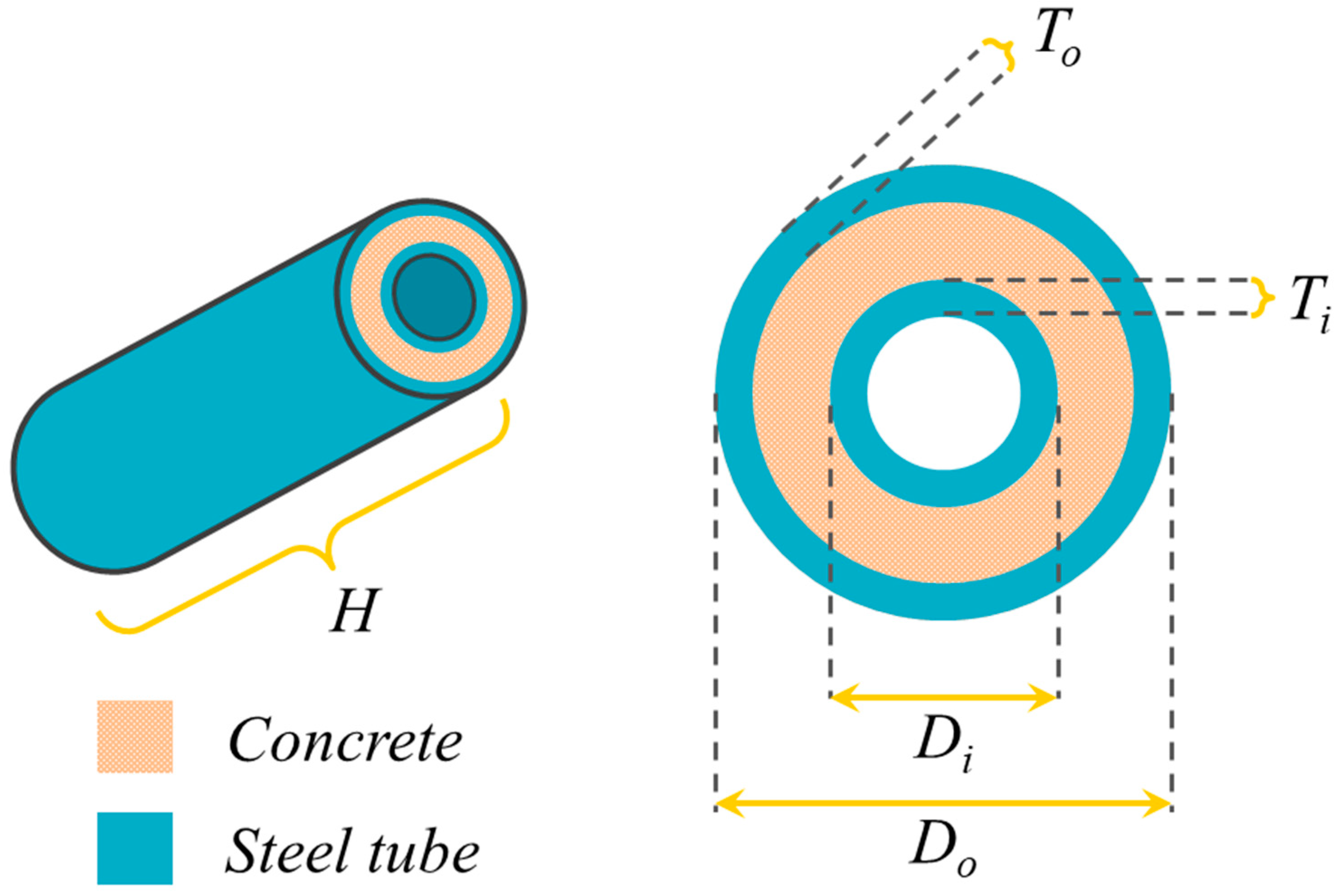
| Variables | Descriptions | Note |
|---|---|---|
| H (mm) | Column length | External dimensions |
| Do (mm) | Diameter of the outer steel tube | |
| Di (mm) | Diameter of the inner steel tube | Internal dimension |
| to (mm) | Thickness of the outer steel tube | Steel tube thickness |
| ti (mm) | Thickness of the inner steel tube | |
| fco (MPa) | Peak strength of unconfined cylinder (d × h = 150 mm × 300 mm) | Concrete strength |
| fyo (MPa) | Yield strength of the outer steel tube | Steel tube strengths |
| fyi (MPa) | Yield strength of the inner steel tube | |
| Nu (kN) | Axial compression capacity | Load-bearing capacity |
| Parameters | Mean | Median | St. D * | Min | Max |
|---|---|---|---|---|---|
| H (mm) | 877.830 | 572.000 | 149.429 | 230.000 | 3502.000 |
| Do (mm) | 220.778 | 165.100 | 32.152 | 74.700 | 603.400 |
| Di (mm) | 129.618 | 76.000 | 25.742 | 33.500 | 477.000 |
| to (mm) | 3.097 | 3.000 | 0.350 | 0.590 | 8.000 |
| ti (mm) | 2.735 | 2.850 | 0.335 | 0.550 | 8.000 |
| fco (MPa) | 40.813 | 37.500 | 4.094 | 18.700 | 74.700 |
| fyo (MPa) | 362.696 | 350.000 | 20.736 | 177.000 | 549.000 |
| fyi (MPa) | 335.807 | 324.000 | 15.434 | 205.000 | 512.000 |
| Nu (kN) | 2095.051 | 1574.000 | 413.341 | 283.000 | 8950.000 |
| Inputs | Outputs |
|---|---|
| H, Do, to, fyo, Nu | Di, ti, fyi, fco |
| Statistical Indicators | Expressions |
|---|---|
| Coefficient of determination (R2) | |
| Root mean square error (RMSE) | |
| Relative root mean squared error (RRMSE) | |
| Performance index (ρ) |
| MTL Models | Hyper-Parameters | Values |
|---|---|---|
| Multi-task Lasso | Regularization parameter λ | 0.091 |
| VSTG | Regularization parameter λ1 | 0.15 |
| Regularization parameter λ2 | 0.14 | |
| Regularization parameter μ | 1.25 | |
| k (k-support norm) | 2 | |
| Number of latent bases M | 3 | |
| MLS-SVR | Regularization parameter λ | 2.013 |
| Regularization parameter β | 33.571 | |
| Kernel function | ERBF | |
| Kernel function parameter σ | 4.493 |
| Outputs | Dataset | R2 | RMSE | RRMSE | ρ |
|---|---|---|---|---|---|
| Di | Trn | 0.926 | 30.542 | 0.240 | 0.122 |
| Tst | 0.904 | 34.905 | 0.275 | 0.141 | |
| ti | Trn | 0.648 | 0.866 | 0.312 | 0.173 |
| Tst | 0.896 | 0.497 | 0.179 | 0.092 | |
| fyi | Trn | 0.258 | 56.611 | 0.166 | 0.11 |
| Tst | 0.457 | 49.811 | 0.146 | 0.087 | |
| fco | Trn | 0.382 | 13.915 | 0.306 | 0.189 |
| Tst | 0.389 | 13.627 | 0.299 | 0.184 |
| Outputs | Dataset | R2 | RMSE | RRMSE | ρ |
|---|---|---|---|---|---|
| Di | Trn | 0.922 | 31.210 | 0.245 | 0.125 |
| Tst | 0.900 | 35.709 | 0.280 | 0.144 | |
| ti | Trn | 0.646 | 0.870 | 0.308 | 0.171 |
| Tst | 0.898 | 0.513 | 0.182 | 0.093 | |
| fyi | Trn | 0.136 | 61.320 | 0.176 | 0.128 |
| Tst | 0.296 | 56.909 | 0.163 | 0.106 | |
| fco | Trn | 0.355 | 14.190 | 0.317 | 0.199 |
| Tst | 0.390 | 13.473 | 0.301 | 0.186 |
| Outputs | Dataset | R2 | RMSE | RRMSE | ρ |
|---|---|---|---|---|---|
| Di | Trn | 0.998 | 5.265 | 0.044 | 0.022 |
| Tst | 0.966 | 20.287 | 0.169 | 0.085 | |
| ti | Trn | 0.973 | 0.239 | 0.093 | 0.047 |
| Tst | 0.906 | 0.392 | 0.152 | 0.078 | |
| fyi | Trn | 0.987 | 7.518 | 0.022 | 0.011 |
| Tst | 0.965 | 12.633 | 0.037 | 0.019 | |
| fco | Trn | 0.975 | 2.754 | 0.064 | 0.032 |
| Tst | 0.866 | 6.499 | 0.150 | 0.078 |
Disclaimer/Publisher’s Note: The statements, opinions and data contained in all publications are solely those of the individual author(s) and contributor(s) and not of MDPI and/or the editor(s). MDPI and/or the editor(s) disclaim responsibility for any injury to people or property resulting from any ideas, methods, instructions or products referred to in the content. |
© 2024 by the authors. Licensee MDPI, Basel, Switzerland. This article is an open access article distributed under the terms and conditions of the Creative Commons Attribution (CC BY) license (https://creativecommons.org/licenses/by/4.0/).
Share and Cite
Wang, Z.; Zhou, J.; Peng, K. The Potential of Multi-Task Learning in CFDST Design: Load-Bearing Capacity Design with Three MTL Models. Materials 2024, 17, 1994. https://doi.org/10.3390/ma17091994
Wang Z, Zhou J, Peng K. The Potential of Multi-Task Learning in CFDST Design: Load-Bearing Capacity Design with Three MTL Models. Materials. 2024; 17(9):1994. https://doi.org/10.3390/ma17091994
Chicago/Turabian StyleWang, Zhenyu, Jian Zhou, and Kang Peng. 2024. "The Potential of Multi-Task Learning in CFDST Design: Load-Bearing Capacity Design with Three MTL Models" Materials 17, no. 9: 1994. https://doi.org/10.3390/ma17091994