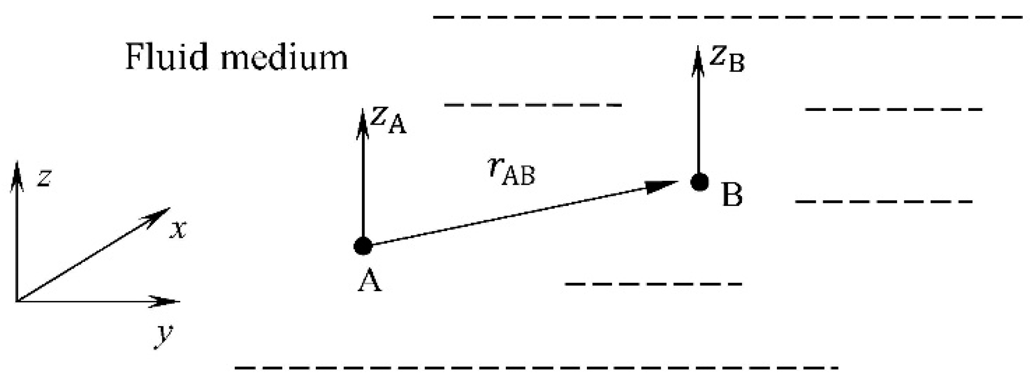
Figure 1.
Determination of the fluid velocity potential.
Figure 1.
Determination of the fluid velocity potential.
Figure 2.
Designations of rectangular subsurface for the fluid.
Figure 2.
Designations of rectangular subsurface for the fluid.
Figure 3.
A system of two plates placed in one plane and immersed in fluid.
Figure 3.
A system of two plates placed in one plane and immersed in fluid.
Figure 4.
A system of two plates placed one above another and immersed in fluid.
Figure 4.
A system of two plates placed one above another and immersed in fluid.
Figure 5.
Designations used in the assembly of the set of algebraic equations.
Figure 5.
Designations used in the assembly of the set of algebraic equations.
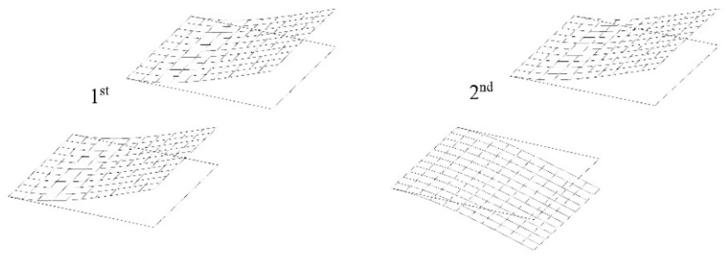
Figure 6.
The set of the finite difference points dividing the single plate area.
Figure 6.
The set of the finite difference points dividing the single plate area.
Figure 7.
Two modes of two cantilever plates immersed in a fluid and placed in one plane along one line for the BEM-BEM solution.
Figure 7.
Two modes of two cantilever plates immersed in a fluid and placed in one plane along one line for the BEM-BEM solution.
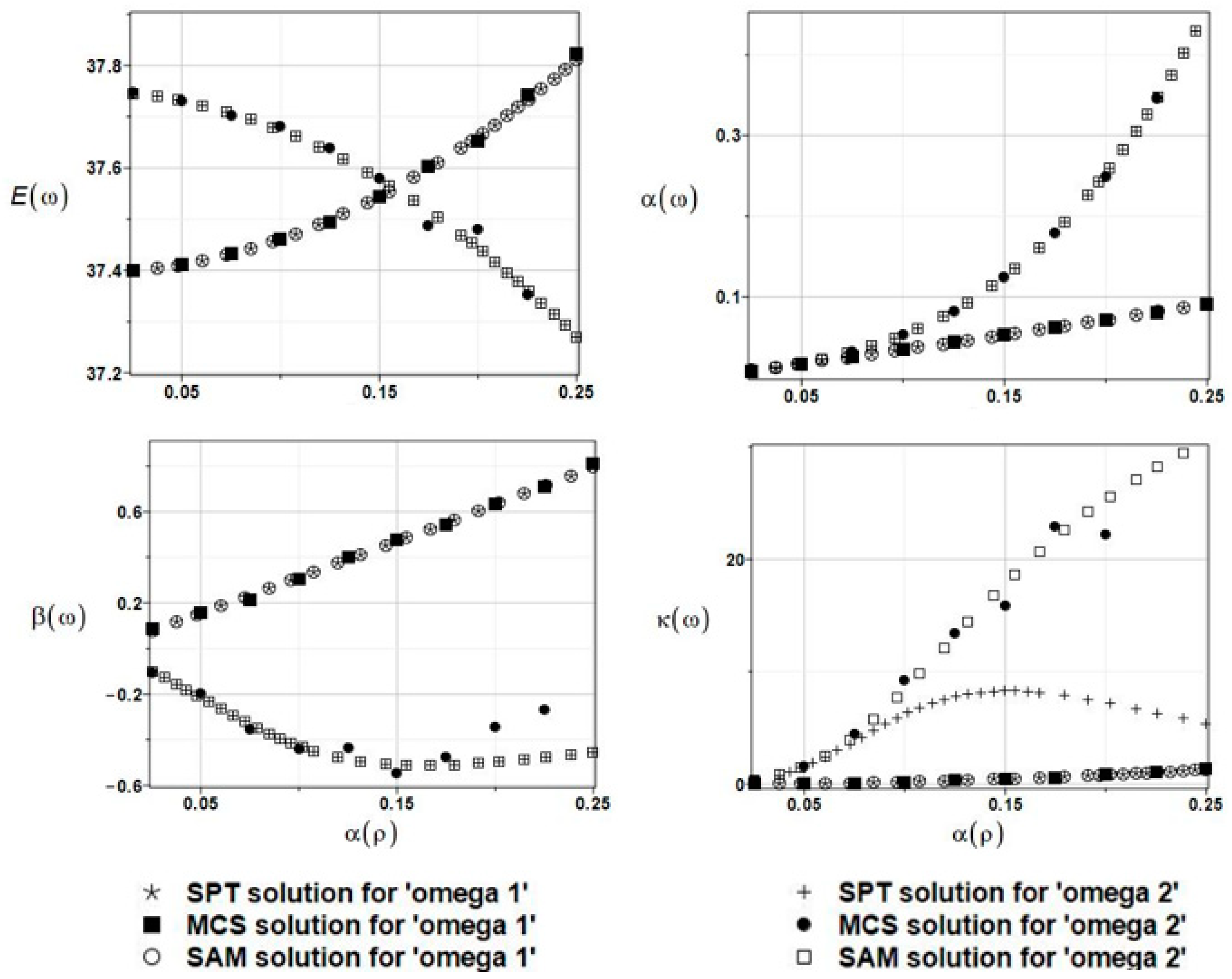
Figure 8.
The results of the first and second natural frequencies, ω1 and ω2, with randomly distributed placement parameter a, BEM-BEM analysis.
Figure 8.
The results of the first and second natural frequencies, ω1 and ω2, with randomly distributed placement parameter a, BEM-BEM analysis.
Figure 9.
The results for the first and second natural frequencies, ω1 and ω2, with randomly distributed fluid density ρf, BEM-BEM analysis.
Figure 9.
The results for the first and second natural frequencies, ω1 and ω2, with randomly distributed fluid density ρf, BEM-BEM analysis.
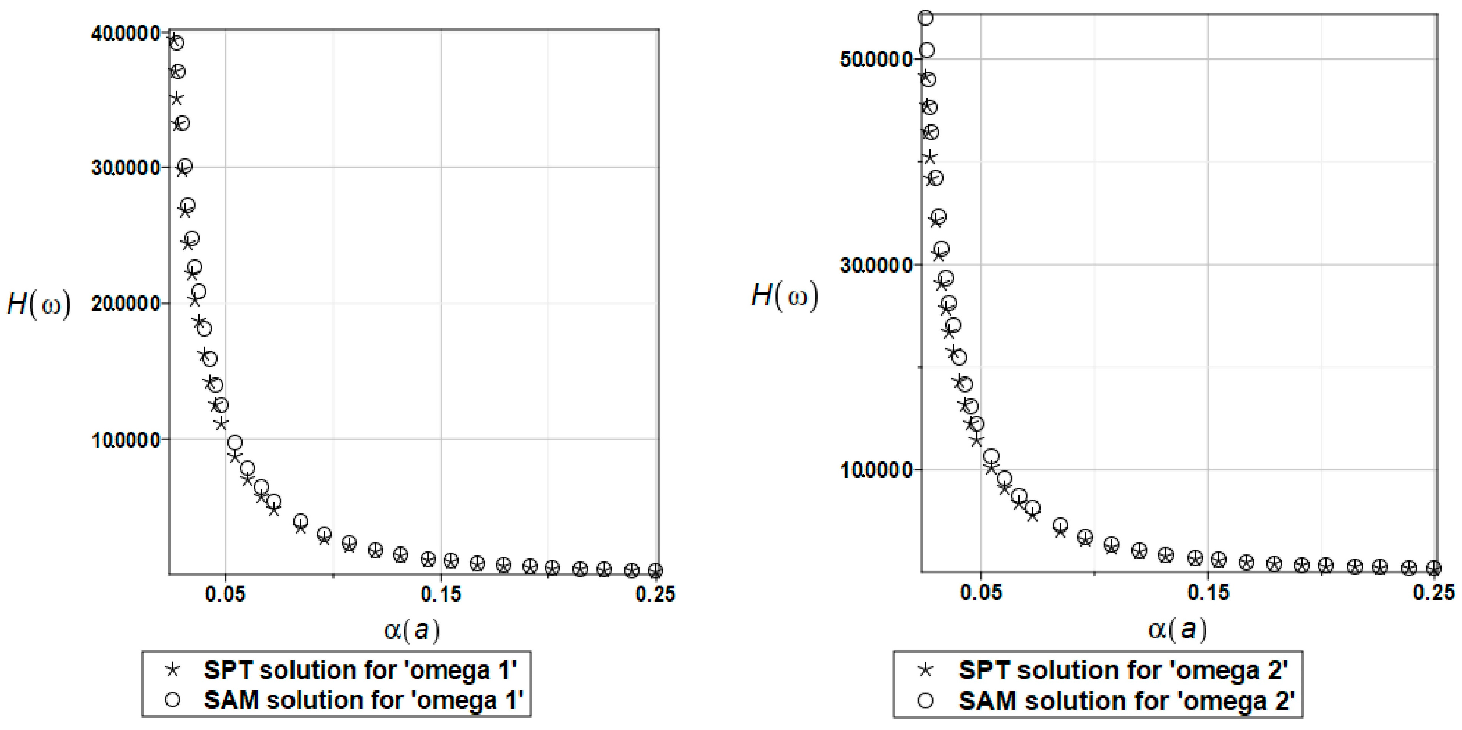
Figure 10.
The results from the first and second natural frequencies, ω1 and ω2, with a randomly distributed collocation point placement parameter , BEM-BEM analysis.
Figure 10.
The results from the first and second natural frequencies, ω1 and ω2, with a randomly distributed collocation point placement parameter , BEM-BEM analysis.
Figure 11.
The propagation of the unsupported segment is described by the parameter “s”.
Figure 11.
The propagation of the unsupported segment is described by the parameter “s”.
Figure 12.
The results for the first and second natural frequencies, ω1 and ω2, with randomly distributed boundary support along the clamped edge, described by the parameter s, BEM-BEM analysis.
Figure 12.
The results for the first and second natural frequencies, ω1 and ω2, with randomly distributed boundary support along the clamped edge, described by the parameter s, BEM-BEM analysis.
Figure 13.
The results for the first and second natural frequencies, ω1 and ω2, with randomly distributed plate thickness h, BEM-BEM analysis.
Figure 13.
The results for the first and second natural frequencies, ω1 and ω2, with randomly distributed plate thickness h, BEM-BEM analysis.
Figure 14.
The results for the first and second natural frequencies, ω1 and ω2, with randomly distributed fluid density ρf, FEM-BEM analysis.
Figure 14.
The results for the first and second natural frequencies, ω1 and ω2, with randomly distributed fluid density ρf, FEM-BEM analysis.
Figure 15.
The results for the first and second natural frequencies, ω1 and ω2, with randomly distributed fluid density ρf, FDM-BEM analysis.
Figure 15.
The results for the first and second natural frequencies, ω1 and ω2, with randomly distributed fluid density ρf, FDM-BEM analysis.
Figure 16.
Two modes of two cantilever plates immersed in fluid and placed one above another for BEM-BEM solution.
Figure 16.
Two modes of two cantilever plates immersed in fluid and placed one above another for BEM-BEM solution.
Figure 17.
The results for the first and second natural frequencies, ω1 and ω2, with randomly distributed location parameter c, BEM-BEM analysis.
Figure 17.
The results for the first and second natural frequencies, ω1 and ω2, with randomly distributed location parameter c, BEM-BEM analysis.
Figure 18.
The results for the first and second natural frequencies, ω1 and ω2, with randomly distributed fluid density ρf, BEM-BEM analysis.
Figure 18.
The results for the first and second natural frequencies, ω1 and ω2, with randomly distributed fluid density ρf, BEM-BEM analysis.
Figure 19.
The results for the first and second natural frequencies, ω1 and ω2, with randomly distributed placement parameter c, FEM-BEM analysis.
Figure 19.
The results for the first and second natural frequencies, ω1 and ω2, with randomly distributed placement parameter c, FEM-BEM analysis.
Figure 20.
The results for the first and second natural frequencies, ω1 and ω2, with randomly distributed placement parameter c, FDM-BEM analysis.
Figure 20.
The results for the first and second natural frequencies, ω1 and ω2, with randomly distributed placement parameter c, FDM-BEM analysis.
Figure 21.
The probabilistic relative entropy with randomly distributed distance parameter a, BEM-BEM analysis.
Figure 21.
The probabilistic relative entropy with randomly distributed distance parameter a, BEM-BEM analysis.
Figure 22.
The safety measure for the first and second natural frequencies and randomly distributed distance parameter a, BEM-BEM analysis.
Figure 22.
The safety measure for the first and second natural frequencies and randomly distributed distance parameter a, BEM-BEM analysis.
Figure 23.
The probabilistic relative entropy for randomly distributed fluid density, FEM-BEM approach.
Figure 23.
The probabilistic relative entropy for randomly distributed fluid density, FEM-BEM approach.
Figure 24.
The probabilistic safety measure for randomly distributed fluid density, FEM-BEM analysis.
Figure 24.
The probabilistic safety measure for randomly distributed fluid density, FEM-BEM analysis.
Figure 25.
The probabilistic relative entropy for randomly distributed fluid density, FDM-BEM analysis.
Figure 25.
The probabilistic relative entropy for randomly distributed fluid density, FDM-BEM analysis.
Figure 26.
The probabilistic safety measure for randomly distributed fluid density, FDM-BEM analysis.
Figure 26.
The probabilistic safety measure for randomly distributed fluid density, FDM-BEM analysis.
Table 1.
The influence of the parameter on the successive natural frequencies for a single cantilever plate fully immersed in water.
Table 1.
The influence of the parameter on the successive natural frequencies for a single cantilever plate fully immersed in water.
| Natural Frequencies ω [rad/s] |
|---|
| BEM-BEM—Present | Anal. Solution [44] | FEM-BEM [48] | FDM-BEM [48] |
|---|
| ω1 | ω2 | ω1 | ω2 | ω1 | ω2 | ω1 | ω2 |
|---|
| 0.001 | 37.582 | 105.379 | 34.9110 | 114.185 | 38.716 | 108.985 | 38.146 | 117.352 |
| 0.01 | 37.540 | 105.262 |
| 0.02 | 37.536 | 105.340 |
Table 2.
Influence of the parameter on the successive natural frequencies for the system of two cantilever plates fully immersed in water and a = 1.0 m.
Table 2.
Influence of the parameter on the successive natural frequencies for the system of two cantilever plates fully immersed in water and a = 1.0 m.
| Natural Frequencies ω [Rad/s], BEM-BEM—Present |
|---|
| [m]
| 0.0001 | 0.00025 | 0.0005 | 0.001 | 0.005 | 0.025 |
|---|
| ω1 | 37.403 | 37.401 | 37.398 | 37.393 | 37.353 | 37.346 |
| ω2 | 37.731 | 37.730 | 37.727 | 37.721 | 37.681 | 37.674 |
| ω3 | 105.187 | 105.185 | 105.171 | 105.151 | 105.026 | 105.108 |
| ω4 | 105.427 | 105.425 | 105.411 | 105.391 | 105.266 | 105.347 |
Table 3.
Natural frequencies for the system of two cantilever plates fully immersed in water and a = 1.0 m obtained for the FEM-BEM and FDM-BEM approaches.
Table 3.
Natural frequencies for the system of two cantilever plates fully immersed in water and a = 1.0 m obtained for the FEM-BEM and FDM-BEM approaches.
| Natural Frequencies ω [Rad/s] |
|---|
| FEM-BEM—Present | FDM-BEM—Present |
|---|
| ω1 | ω2 | ω3 | ω4 | ω1 | ω2 | ω3 | ω4 |
| 38.238 | 38.552 | 107.693 | 107.916 | 38.537 | 38.854 | 116.047 | 116.295 |
Table 4.
The comparison of the results obtained from the system of two cantilever plates fully immersed in water and a = 1.0 m under the FEM-BEM approach and three different FEM and BEM meshes.
Table 4.
The comparison of the results obtained from the system of two cantilever plates fully immersed in water and a = 1.0 m under the FEM-BEM approach and three different FEM and BEM meshes.
| Plate FEM mesh | | | |
| Fluid BEM mesh | | | |
| 37.567 | 38.238 | 38.593 |
| 37.896 | 38.552 | 38.898 |
| 105.684 | 107.693 | 108.786 |
| 105.924 | 107.916 | 109.000 |
Table 5.
The comparison of the results obtained from the system of two cantilever plates fully immersed in water and a =1.0 m under the FDM-BEM approach, three different FDM grids, and BEM meshes.
Table 5.
The comparison of the results obtained from the system of two cantilever plates fully immersed in water and a =1.0 m under the FDM-BEM approach, three different FDM grids, and BEM meshes.
| Plate FDM grid | | | |
| Fluid BEM mesh | | | |
| 36.557 | 37.979 | 38.537 |
| 36.939 | 38.312 | 38.854 |
| 121.223 | 117.230 | 116.047 |
| 121.586 | 117.509 | 116.295 |
Table 6.
An influence of the parameter on the natural frequency ω for the system of two cantilever plates completely immersed in water and a = 1.0 m.
Table 6.
An influence of the parameter on the natural frequency ω for the system of two cantilever plates completely immersed in water and a = 1.0 m.
| Natural Frequencies ω [Rad/s] BEM-BEM—Present |
|---|
| [m] | 0.0001 | 0.00025 | 0.0005 | 0.001 | 0.005 | 0.025 |
| ω1 | 35.792 | 35.790 | 35.787 | 35.781 | 35.743 | 35.736 |
| ω2 | 39.071 | 39.069 | 39.066 | 39.059 | 39.018 | 39.012 |
| ω3 | 103.723 | 103.721 | 103.707 | 103.687 | 103.564 | 103.644 |
| ω4 | 106.788 | 106.286 | 106.771 | 106.751 | 106.624 | 106.707 |
Table 7.
Natural frequencies ω for the system of two cantilever plates fully immersed in water and c = 1.0 m obtained for FEM-BEM and FDM-BEM approaches.
Table 7.
Natural frequencies ω for the system of two cantilever plates fully immersed in water and c = 1.0 m obtained for FEM-BEM and FDM-BEM approaches.
| Natural Frequencies ω [Rad/s] |
|---|
| FEM-BEM—Present | FDM-BEM—Present |
|---|
| ω1 | ω2 | ω3 | ω4 | ω1 | ω2 | ω3 | ω4 |
|---|
| 36.658 | 39.867 | 106.292 | 109.219 | 36.935 | 40.188 | 114.487 | 117.746 |
Table 8.
The comparison of the results from the system of two cantilever plates fully immersed in water, c = 1.0 m obtained using the FEM-BEM approach, and three different FEM and BEM meshes.
Table 8.
The comparison of the results from the system of two cantilever plates fully immersed in water, c = 1.0 m obtained using the FEM-BEM approach, and three different FEM and BEM meshes.
| Plate FEM mesh | | | |
| Fluid BEM mesh | | | |
| 35.950 | 36.658 | 37.029 |
| 39.238 | 39.867 | 40.201 |
| 104.218 | 106.292 | 107.417 |
| 107.286 | 109.219 | 110.274 |
Table 9.
The comparison of the results from system of two cantilever plates fully immersed in water, c = 1.0 m obtained using the FDM-BEM approach, and three different FDM grids and BEM meshes.
Table 9.
The comparison of the results from system of two cantilever plates fully immersed in water, c = 1.0 m obtained using the FDM-BEM approach, and three different FDM grids and BEM meshes.
| Plate FDM grid | | | |
| Fluid BEM mesh | | | |
| 34.755 | 36.332 | 36.935 |
| 38.429 | 39.682 | 40.188 |
| 119.050 | 115.530 | 114.487 |
| 123.599 | 119.089 | 117.746 |


