
The Effect of Copper–Graphene Composite Architecture on Thermal Transport Efficiency

 ,
,  ,
,
Abstract
:
1. Introduction
2. Materials and Methods
3. Results and Discussion
4. Conclusions
Author Contributions
Funding
Institutional Review Board Statement
Informed Consent Statement
Data Availability Statement
Conflicts of Interest
References
- Wang, X.; Xiao, W.; Wang, J.; Sun, L.; Shi, J.; Guo, H.; Liu, Y.; Wang, L. Enhanced interfacial strength of graphene reinforced aluminum composites via X (Cu, Ni, Ti)-coating: Molecular-dynamics insights. Adv. Powder Technol. 2021, 32, 2585–2590. [Google Scholar] [CrossRef]
- Safina, L.R.; Baimova, J.A.; Krylova, K.A.; Murzaev, R.T.; Shcherbinin, S.A.; Mulyukov, R.R. Ni–Graphene Composite Obtained by Pressure–Temperature Treatment: Atomistic Simulations. Phys. Status Solidi (RRL)–Rapid Res. Lett. 2021, 15, 2100429. [Google Scholar] [CrossRef]
- Hou, B.; Liu, P.; Wang, A.; Xie, J. Interface optimization strategy for enhancing the mechanical and thermal properties of aligned graphene/Al composite. J. Alloys Compd. 2022, 900, 163555. [Google Scholar] [CrossRef]
- Wang, M.; Sheng, J.; Wang, L.D.; Wang, G.; Fei, W.D. Achieving high strength and electrical properties in drawn fine Cu matrix composite wire reinforced by in-situ grown graphene. J. Mater. Res. Technol. 2022, 17, 3205–3210. [Google Scholar] [CrossRef]
- Wu, M.; Chen, Z.; Huang, C.; Huang, K.; Jiang, K.; Liu, J. Graphene platelet reinforced copper composites for improved tribological and thermal properties. RSC Adv. 2019, 9, 39883–39892. [Google Scholar] [CrossRef] [PubMed]
- Chen, D.; Feng, H.; Li, J. Graphene Oxide: Preparation, Functionalization, and Electrochemical Applications. Chem. Rev. 2012, 112, 6027–6053. [Google Scholar] [CrossRef] [PubMed]
- Wejrzanowski, T.; Grybczuk, M.; Chmielewski, M.; Pietrzak, K.; Kurzydlowski, K.; Strojny-Nedza, A. Thermal conductivity of metal-graphene composites. Mater. Des. 2016, 99, 163–173. [Google Scholar] [CrossRef]
- Guo, S.; Zhang, X.; Shi, C.; Zhao, D.; Liu, E.; He, C.; Zhao, N. Comprehensive performance regulation of Cu matrix composites with graphene nanoplatelets in situ encapsulated Al2O3 nanoparticles as reinforcement. Carbon 2022, 188, 81–94. [Google Scholar] [CrossRef]
- Ali, S.; Ahmad, F.; Yusoff, P.S.M.M.; Muhamad, N.; Oñate, E.; Raza, M.R.; Malik, K. A review of graphene reinforced Cu matrix composites for thermal management of smart electronics. Compos. Part A Appl. Sci. Manuf. 2021, 144, 106357. [Google Scholar] [CrossRef]
- Zhai, W.; Lu, W.; Chen, Y.; Liu, X.; Zhou, L.; Lin, D. Gas-atomized copper-based particles encapsulated in graphene oxide for high wear-resistant composites. Compos. Part B Eng. 2019, 157, 131–139. [Google Scholar] [CrossRef]
- Zhang, J.; Xu, Q.; Gao, L.; Ma, T.; Qiu, M.; Hu, Y.; Wang, H.; Luo, J. A molecular dynamics study of lubricating mechanism of graphene nanoflakes embedded in Cu-based nanocomposite. Appl. Surf. Sci. 2020, 511, 145620. [Google Scholar] [CrossRef]
- Lin, G.; Peng, Y.; Dong, Z.; Xiong, D.B. Tribology behavior of high-content graphene/nanograined Cu bulk composites from core/shell nanoparticles. Compos. Commun. 2021, 25, 100777. [Google Scholar] [CrossRef]
- Zhang, X.; Xu, Y.; Wang, M.; Liu, E.; Zhao, N.; Shi, C.; Lin, D.; Zhu, F.; He, C. A powder-metallurgy-based strategy toward three-dimensional graphene-like network for reinforcing copper matrix composites. Nat. Commun. 2020, 11, 2775. [Google Scholar] [CrossRef] [PubMed]
- Shi, L.; Liu, M.; Yang, Y.; Liu, R.; Zhang, W.; Zheng, Q.; Ren, Z. Achieving high strength and ductility in copper matrix composites with graphene network. Mater. Sci. Eng. A 2021, 828, 142107. [Google Scholar] [CrossRef]
- Shi, L.; Liu, M.; Zhang, W.; Ren, W.; Zhou, S.; Zhou, Q.; Yang, Y.; Ren, Z. Interfacial Design of Graphene Nanoplate Reinforced Copper Matrix Composites for High Mechanical Performance. JOM 2022, 74, 3082–3090. [Google Scholar] [CrossRef]
- Navik, R.; Ding, X.; Huijun, T.; Gai, Y.; Zhao, Y. Fabrication of copper nanowire and hydroxylated graphene hybrid with high conductivity and excellent stability. Appl. Mater. Today 2020, 19, 100619. [Google Scholar] [CrossRef]
- Omran, H.; Eivani, A.R.; Farbakhti, M.; Jafarian, H.R. Tribological properties of copper-graphene (CuG) composite fabricated by accumulative roll bonding. J. Mater. Res. Technol. 2023, 25, 4650–4657. [Google Scholar] [CrossRef]
- Jamadon, N.; Rasid, N.; Ahmad, M.A.; Lutfi, M.; Adzila, S.; Jamal, N.; Muhamad, N. The Effect of Graphene Addition on the Microstructure and Properties of Graphene/Copper Composites for Sustainable Energy Materials. In Proceedings of the IOP Conference Series: Earth and Environmental Science 2023, Seoul, Republic of Korea, 17–18 November 2022; Volume 1216, p. 012028. [Google Scholar] [CrossRef]
- Lopez-Barajas, F.; Ramos, L.; Sanchez, S.; Ramírez, E.; Martinez, G.; Espinoza-Martínez, A.; da Silva, L.; Gámez, F.; Rodriguez-Fernandez, O.; Beltrán-Ramírez, F.; et al. Epoxy/hybrid graphene-copper nanocomposite materials with enhanced thermal conductivity. J. Appl. Polym. Sci. 2022, 139, e52419. [Google Scholar] [CrossRef]
- Singh, G.; Ghai, V.; Chaudhary, S.; Singh, S.; Agnihotri, P.; Singh, H. Effect of graphene on thermal conductivity of laser cladded copper. Emergent Mater. 2021, 4, 1491–1498. [Google Scholar] [CrossRef]
- Li, X.; Miu, J.; An, M.; Mei, J.; Zheng, F.; Jiang, J.; Wang, H.; Huang, Y.; Li, Q. Preparation of graphene/copper composite with thiophenol molecular junction for thermal conductive application. New J. Chem. 2022, 46, 10107–10116. [Google Scholar] [CrossRef]
- He, S.; Liu, B.; Pei, Z.; Zhang, X.; Liu, B.; Xiong, D.-B. Defect effect of graphene on interface properties of copper/graphene/copper composite: A first-principles study. J. Appl. Phys. 2023, 134, 075104. [Google Scholar] [CrossRef]
- Katin, K.; Kochaev, A.; Berezniczcky, I.; Kalika, E.; Kaya, S.; Flores-Moreno, R.; Maslov, M. Interaction of pristine and novel graphene allotropes with copper nanoparticles: Coupled density functional and molecular dynamics study. Diam. Relat. Mater. 2023, 138, 110190. [Google Scholar] [CrossRef]
- Shelepev, I.A.; Kolesnikov, I.D. 2022 Excitation and propagation of 1-crowdion in bcc niobium lattice. Mater. Technol. Des. 2022, 4, 5–10. [Google Scholar] [CrossRef]
- Yankovskaya, U.I.; Zakharov, P.V. Heat resistance of a Pt crystal reinforced with CNT’s. Mater. Technol. Des. 2021, 3, 64–67. [Google Scholar] [CrossRef]
- Savin, A.V. Multistability of Carbon Nanotube Packings on Flat Substrate. Phys. Status Solidi (RRL)–Rapid Res. Lett. 2021, 16, 2100437. [Google Scholar] [CrossRef]
- Yankovaskaya, U.I.; Korznikova, E.A.; Korpusova, S.D.; Zakharov, P.V. Mechanical Properties of the Pt-CNT Composite under Uniaxial Deformation: Tension and Compression. Materials 2023, 16, 4140. [Google Scholar] [CrossRef]
- Zakharov, P.V.; Korznikova, E.A.; Izosimov, A.A.; Kochkin, A.S. The Influence of Crystal Anisotropy on the Characteristics of Solitary Waves in the Nonlinear Supratransmission Effect: Molecular Dynamic Modeling. Computation 2023, 11, 193. [Google Scholar] [CrossRef]
- Savin, A.V.; Korznikova, E.A.; Dmitriev, S.V.; Soboleva, E.G. Graphene nanoribbon winding around carbon nanotube. Comput. Mater. Sci. 2017, 135, 99–108. [Google Scholar] [CrossRef]
- Hidalgo-Manrique, P.; Lei, X.; Xu, R.; Zhou, M.; Kinloch, I.A.; Young, R.J. Copper/graphene composites: A review. J. Mater. Sci. 2019, 54, 12236–12289. [Google Scholar] [CrossRef]
- Davletshin, A.R.; Ustiuzhanina, S.V.; Kistanov, A.A.; Saadatmand, D.; Dmitriev, S.V.; Zhou, K.; Korznikova, E.A. Electronic structure of graphene– and BN–supported phosphorene. Phys. B Condens. Matter. 2018, 534, 63–67. [Google Scholar] [CrossRef]
- Plimpton, S. Fast parallel algorithms for short-range molecular dynamics. J. Comput. Phys. 1995, 117, 1–19. [Google Scholar] [CrossRef]
- Stukowski, A. Visualization and analysis of atomistic simulation data with OVITO–the Open Visualization Tool. Model. Simul. Mater. Sci. Eng. 2010, 18, 015012. [Google Scholar] [CrossRef]
- Ikeshoji, T.; Hafskjold, B. Non-equilibrium molecular dynamics calculation of heat conduction in liquid and through liquid-gas interface. Mol. Phys. 1994, 81, 251–261. [Google Scholar] [CrossRef]
- Stuart, S.J.; Tutein, A.B.; Harrison, J.A. A reactive potential for hydrocarbons with intermolecular interactions. J. Chem. Phys. 2000, 112, 6472–6486. [Google Scholar] [CrossRef]
- Zhou, X.; Wadley, H.; Johnson, R.; Larson, D.; Tabat, N.; Cerezo, A.; Petford-Long, A.; Smith, G.; Clifton, P.; Martens, R.; et al. Atomic scale structure of sputtered metal multilayers. Acta Mater. 2001, 49, 4005–4015. [Google Scholar] [CrossRef]
- Safina, L.R.; Rozhnova, E.A.; Murzaev, R.T.; Baimova, J.A. Effect of Interatomic Potential on Simulation of Fracture Behavior of Cu/Graphene Composite: A Molecular Dynamics Study. Appl. Sci. 2023, 13, 916. [Google Scholar] [CrossRef]
- Poncharal, P.; Berger, C.; Yi, Y.; Wang, Z.L.; de Heer, W.A. Room Temperature Ballistic Conduction in Carbon Nanotubes. J. Phys. Chem. B 2002, 106, 12104–12118. [Google Scholar] [CrossRef]
- Bachmann, M.D.; Sharpe, A.L.; Baker, G.; Barnard, A.W.; Putzke, C.; Scaffidi, T.; Nandi, N.; McGuinness, P.H.; Zhakina, E.; Moravec, M.; et al. Directional ballistic transport in the two-dimensional metal PdCoO2. Nat. Phys. 2022, 18, 819–824. [Google Scholar] [CrossRef]
- Taleb, A.A.; Farías, D. Phonon dynamics of graphene on metals. J. Phys. Condens. Matter 2016, 28, 103005. [Google Scholar] [CrossRef]
- Smith, D.S.; Puech, F.; Nait-Ali, B.; Alzina, A.; Honda, S. Grain boundary thermal resistance and finite grain size effects for heat conduction through porous polycrystalline alumina. Int. J. Heat Mass Transf. 2018, 121, 1273–1280. [Google Scholar] [CrossRef]
- Zhu, J.; Huang, S.; Xie, Z.; Guo, H.; Yang, H. Thermal Conductance of Copper–Graphene Interface: A Molecular Simulation. Materials 2022, 15, 7588. [Google Scholar] [CrossRef] [PubMed]
- Koltsova, T.; Bobrynina, E.; Vozniakovskii, A.; Larionova, T.; Klimova-Korsmik, O. Thermal Conductivity of Composite Materials Copper-Fullerene Soot. Materials 2022, 15, 1415. [Google Scholar] [CrossRef] [PubMed]
- Wang, L.; Li, J.; Catalano, M.; Bai, G.; Li, N.; Dai, J.; Wang, X.; Zhang, H.; Wang, J.; Kim, M.J. Enhanced thermal conductivity in Cu/diamond composites by tailoring the thickness of interfacial TiC layer. Compos. Part A Appl. Sci. Manuf. 2018, 113, 76–82. [Google Scholar] [CrossRef]
- Monteverde, U.; Pal, J.; Migliorato, M.A.; Missous, M.; Bangert, U.; Zan, R.; Kashtiban, R.; Powell, D. Under pressure: Control of strain, phonons and bandgap opening in rippled graphene. Carbon 2015, 91, 266–274. [Google Scholar] [CrossRef]


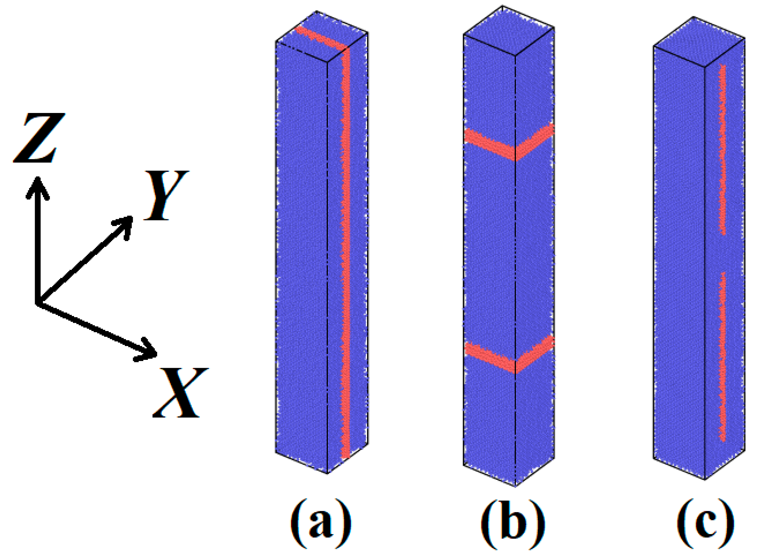
| κ, W/(m·K) | |||||
|---|---|---|---|---|---|
| Number of Graphene Layers | Pure Cu Crystal | Inf. Graphene Layers along the Z Axis | Inf. Graphene Layers Perpendicularly to the Z Axis | 15 nm Graphene Layers | 8 nm Graphene Layers |
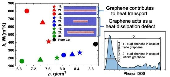
| 1 | 380 | 414.2 | 2.51 | 205.9 | 272.6 |
| 2 | 654.6 | 2.18 | 179.1 | 246.8 | |
| 3 | 803.3 | 1.53 | 163.6 | 240.8 | |
| Volume Fraction | kGr, W/(m·K) | |||||
|---|---|---|---|---|---|---|
| Number of Graphene Layers | Inf. Graphene Layers along the Z Axis | 15 nm Graphene Layers | 8 nm Graphene Layers | Inf. Graphene Layers along the Z Axis | 15 nm Graphene Layers | 8 nm Graphene Layers |
| 1 | 0.104 | 0.085 | 0.047 | 390.0 | 82.1 | 26.2 |
| 2 | 0.154 | 0.128 | 0.066 | 729.3 | 153.5 | 49.0 |
| 3 | 0.208 | 0.188 | 0.095 | 1128.3 | 237.5 | 75.8 |
| Κ′, W/(m·K) | |||
|---|---|---|---|
| Number of Graphene Layers | Inf. Graphene Layers along the Z Axis | 15 nm Graphene Layers | 8 nm Graphene Layers |
| 1 | 381.1 | 354.7 | 363.4 |
| 2 | 433.6 | 353.2 | 358.2 |
| 3 | 535.6 | 351.0 | 351.1 |
Disclaimer/Publisher’s Note: The statements, opinions and data contained in all publications are solely those of the individual author(s) and contributor(s) and not of MDPI and/or the editor(s). MDPI and/or the editor(s) disclaim responsibility for any injury to people or property resulting from any ideas, methods, instructions or products referred to in the content. |
© 2023 by the authors. Licensee MDPI, Basel, Switzerland. This article is an open access article distributed under the terms and conditions of the Creative Commons Attribution (CC BY) license (https://creativecommons.org/licenses/by/4.0/).
Share and Cite
Kazakov, A.M.; Korznikova, G.F.; Tuvalev, I.I.; Izosimov, A.A.; Korznikova, E.A. The Effect of Copper–Graphene Composite Architecture on Thermal Transport Efficiency. Materials 2023, 16, 7199. https://doi.org/10.3390/ma16227199
Kazakov AM, Korznikova GF, Tuvalev II, Izosimov AA, Korznikova EA. The Effect of Copper–Graphene Composite Architecture on Thermal Transport Efficiency. Materials. 2023; 16(22):7199. https://doi.org/10.3390/ma16227199
Chicago/Turabian StyleKazakov, Arseny M., Galiia F. Korznikova, Ilyas I. Tuvalev, Artem A. Izosimov, and Elena A. Korznikova. 2023. "The Effect of Copper–Graphene Composite Architecture on Thermal Transport Efficiency" Materials 16, no. 22: 7199. https://doi.org/10.3390/ma16227199