
Comparison of Various Intrinsic Defect Criteria to Plot Kitagawa–Takahashi Diagrams in Additively Manufactured AlSi10Mg


Abstract
:1. Introduction
2. Materials and Methods
2.1. Experimental Methods
2.2. Finite Element Model
2.3. Theory and Calculations
2.3.1. Intrinsic Defect Length Calculation
2.3.2. Correction Factor Hypothesis
2.3.3. Critical Stress Intensity Factor Calculation
2.3.4. Fatigue Life Calculation
3. Results
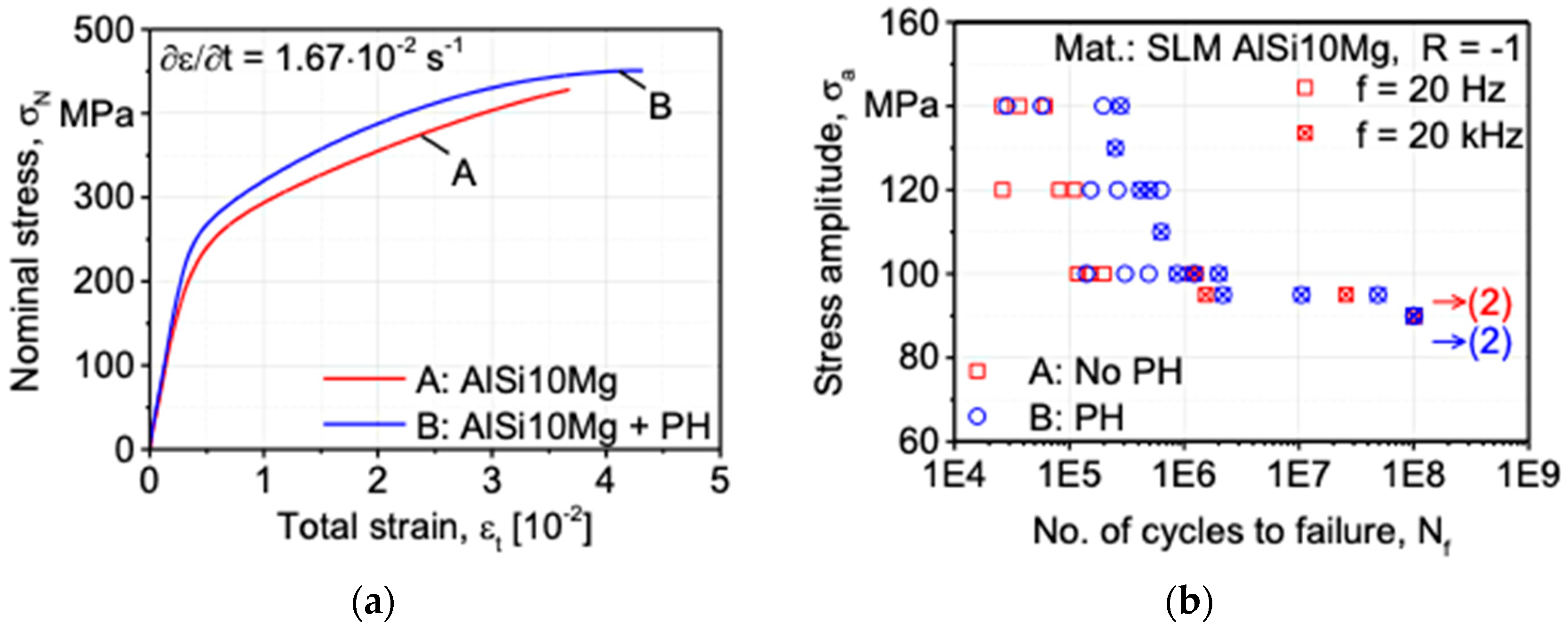
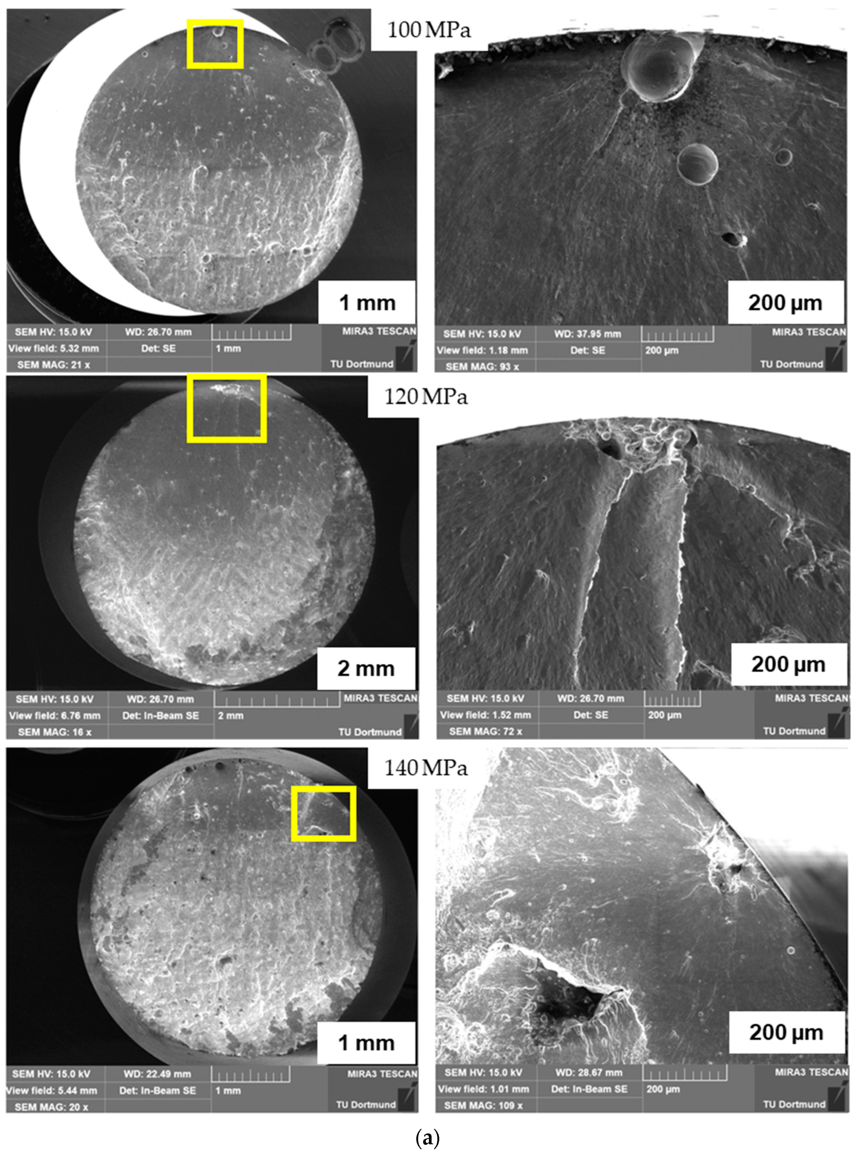
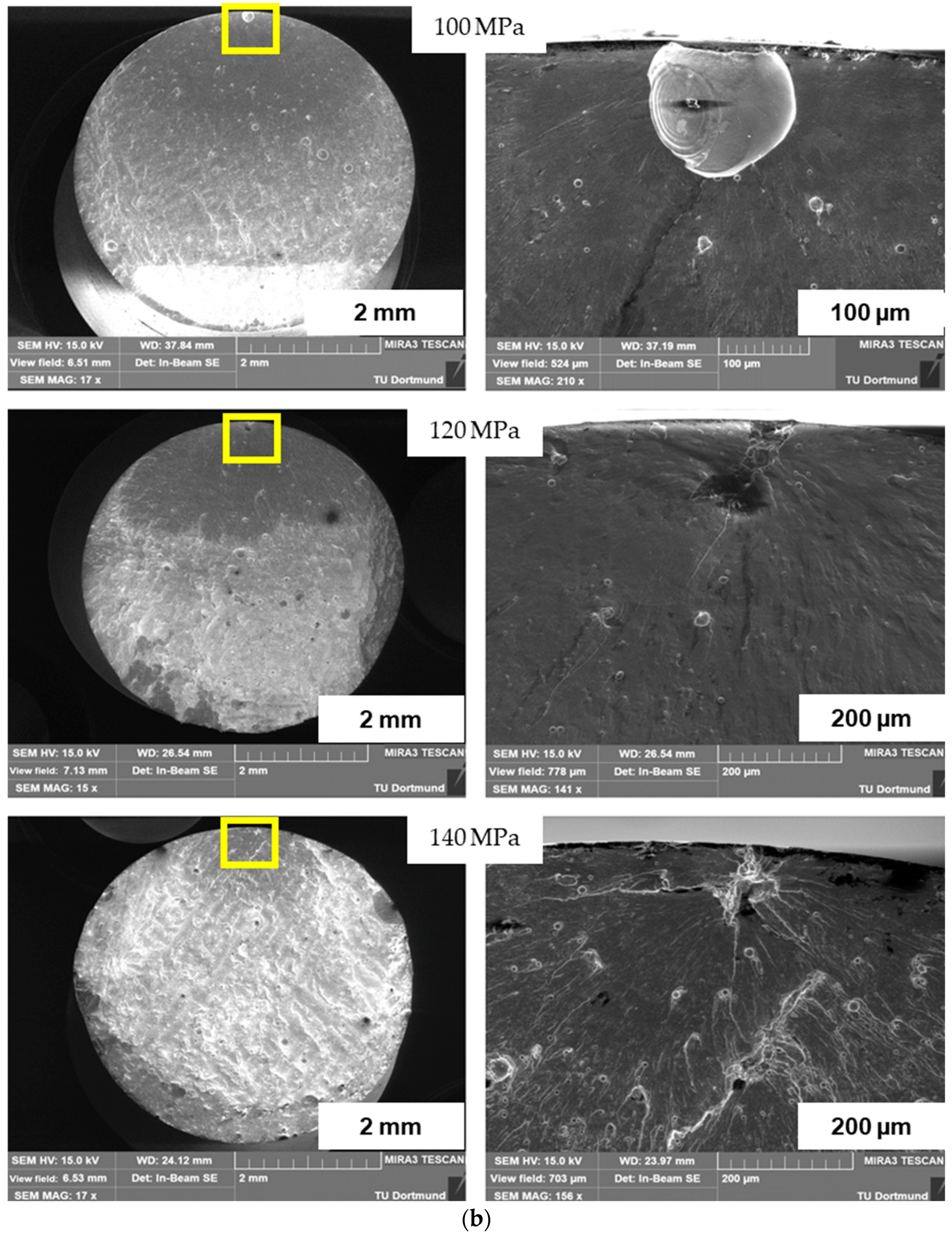
3.1. Experimental Results
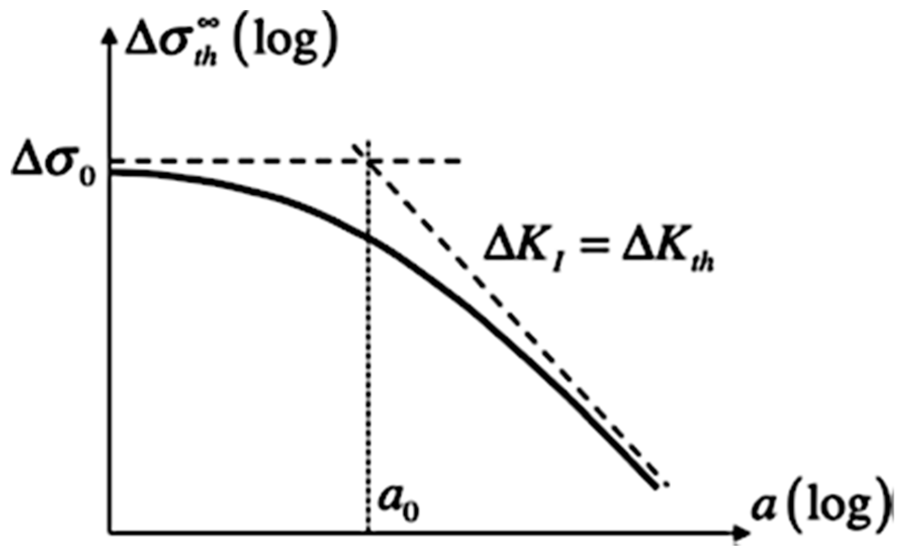
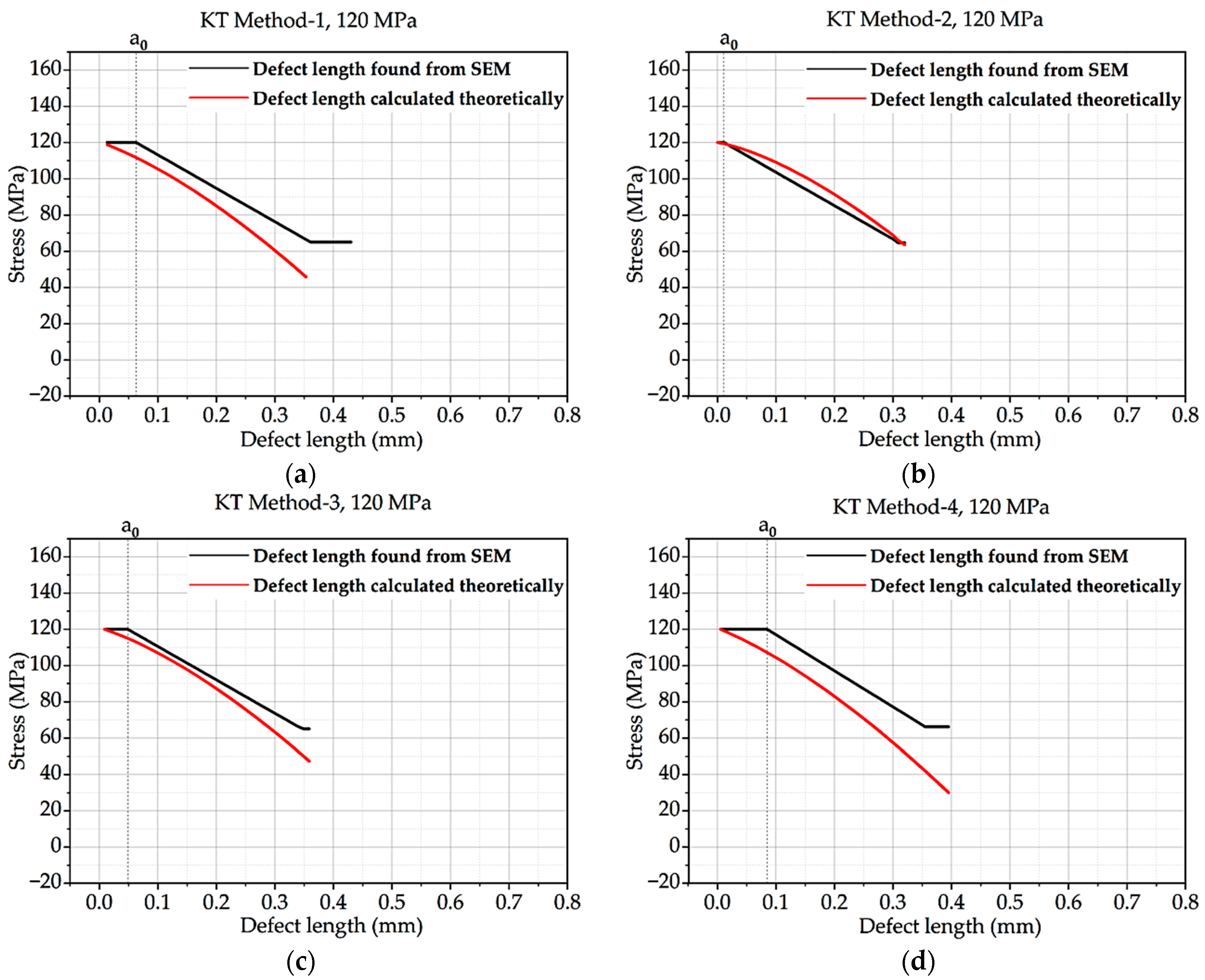
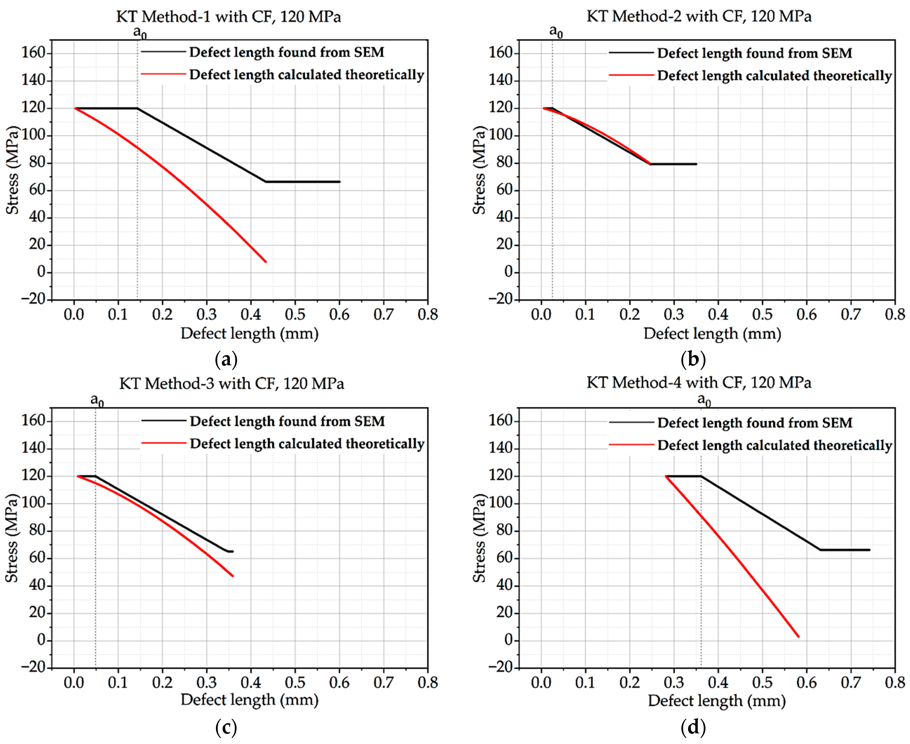
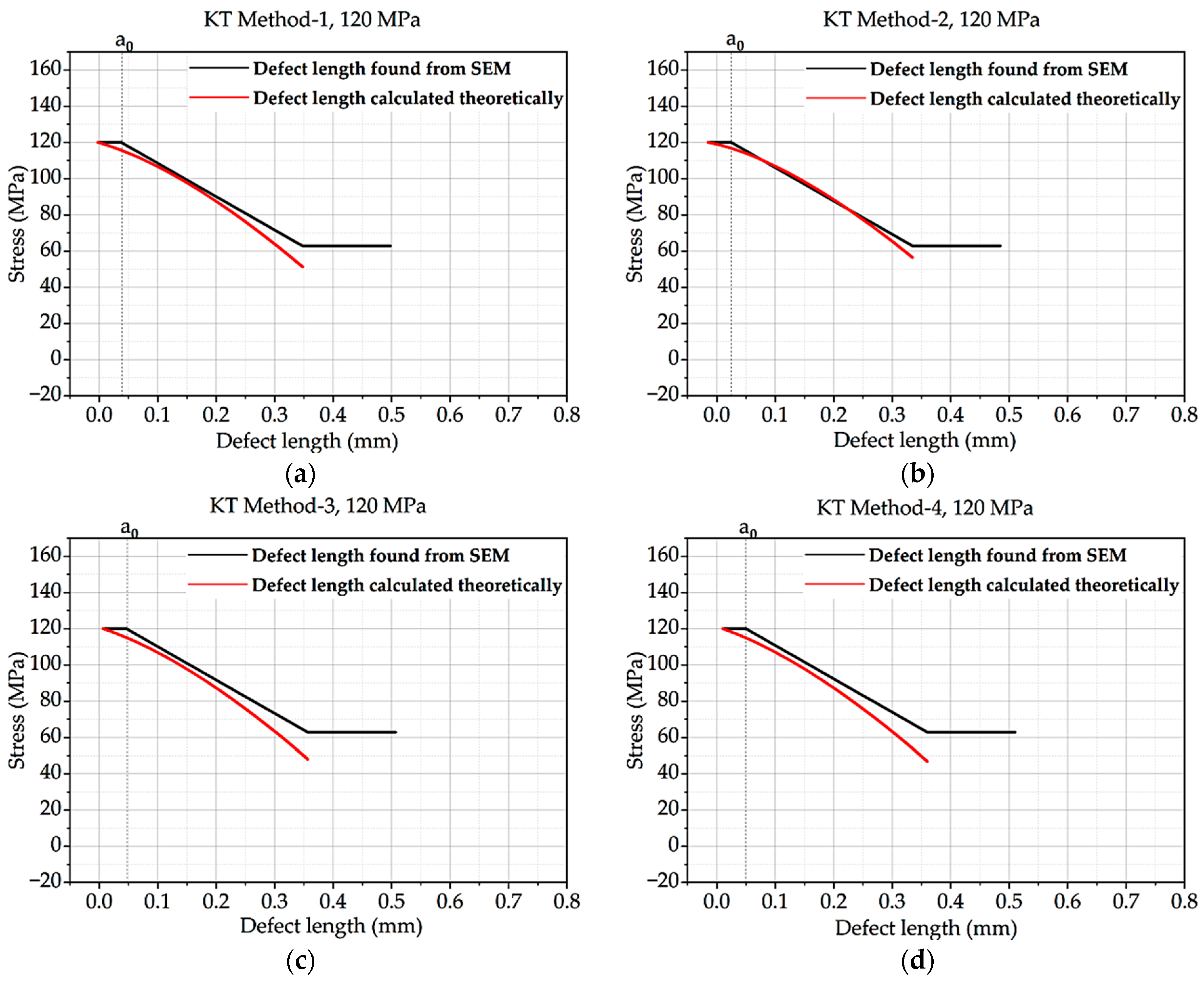
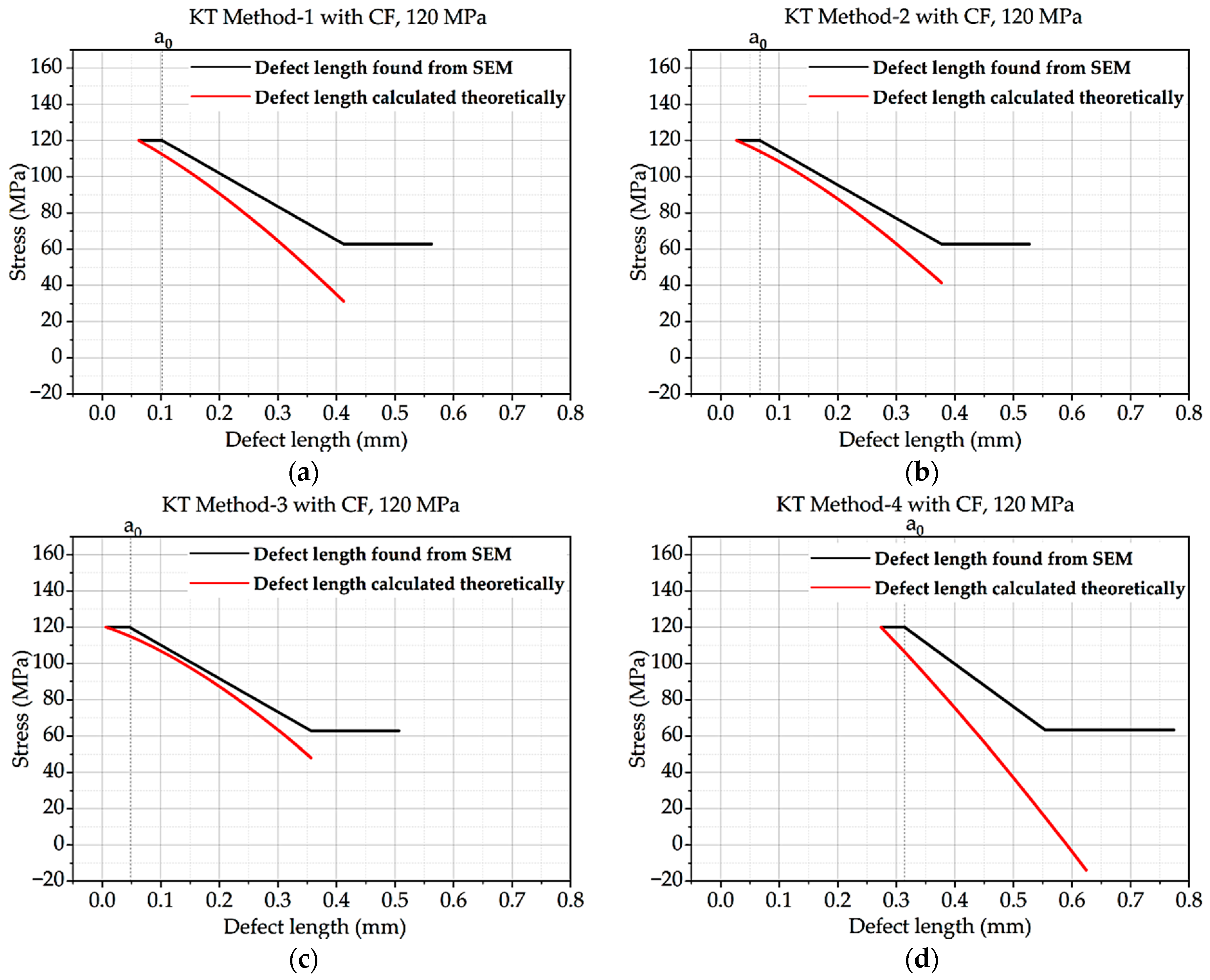
3.2. Kitagawa–Takahashi Diagram Development
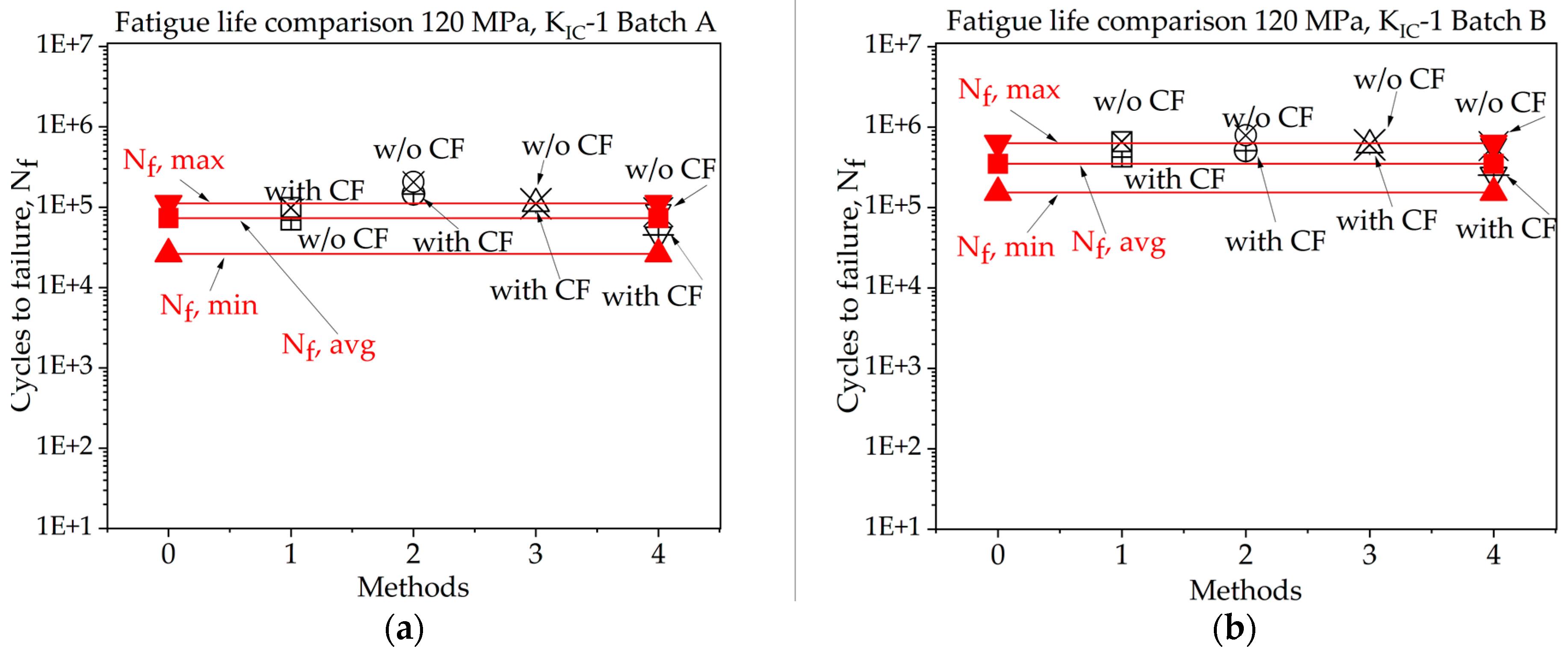
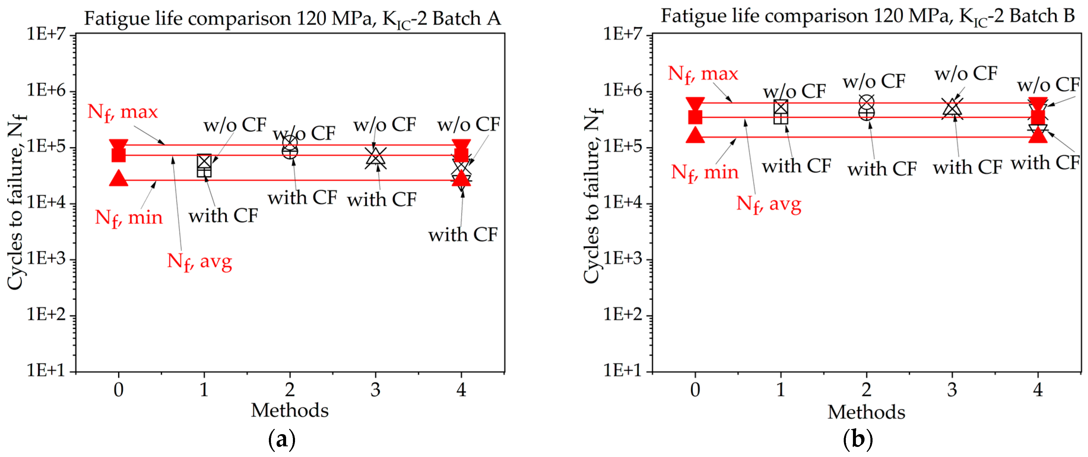
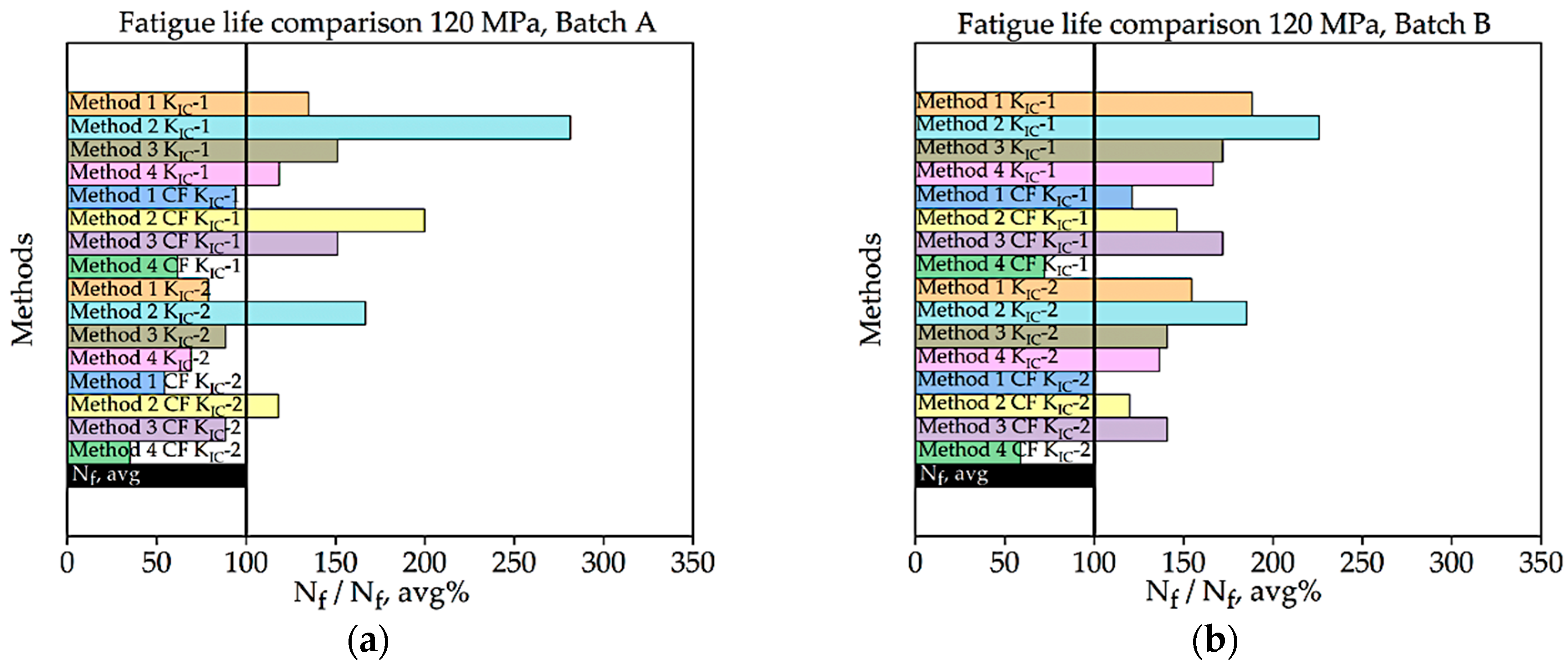
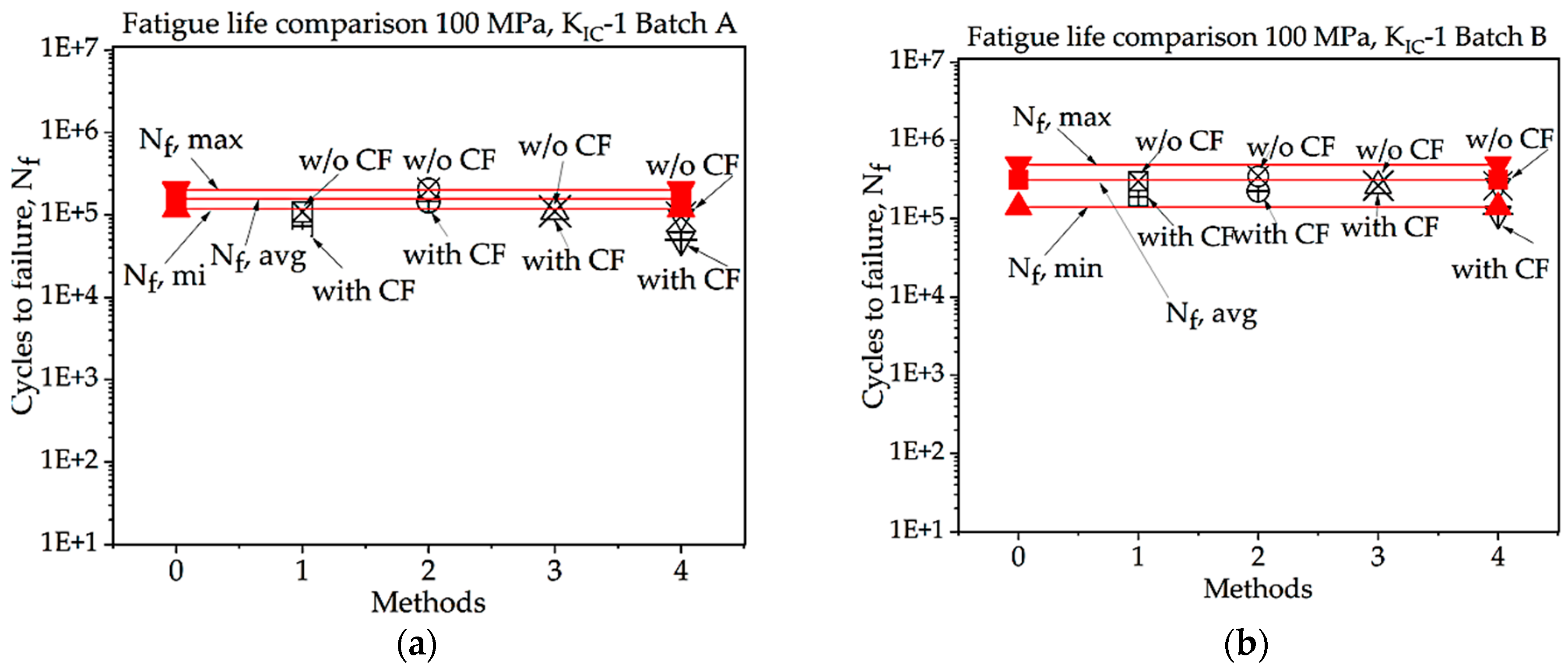
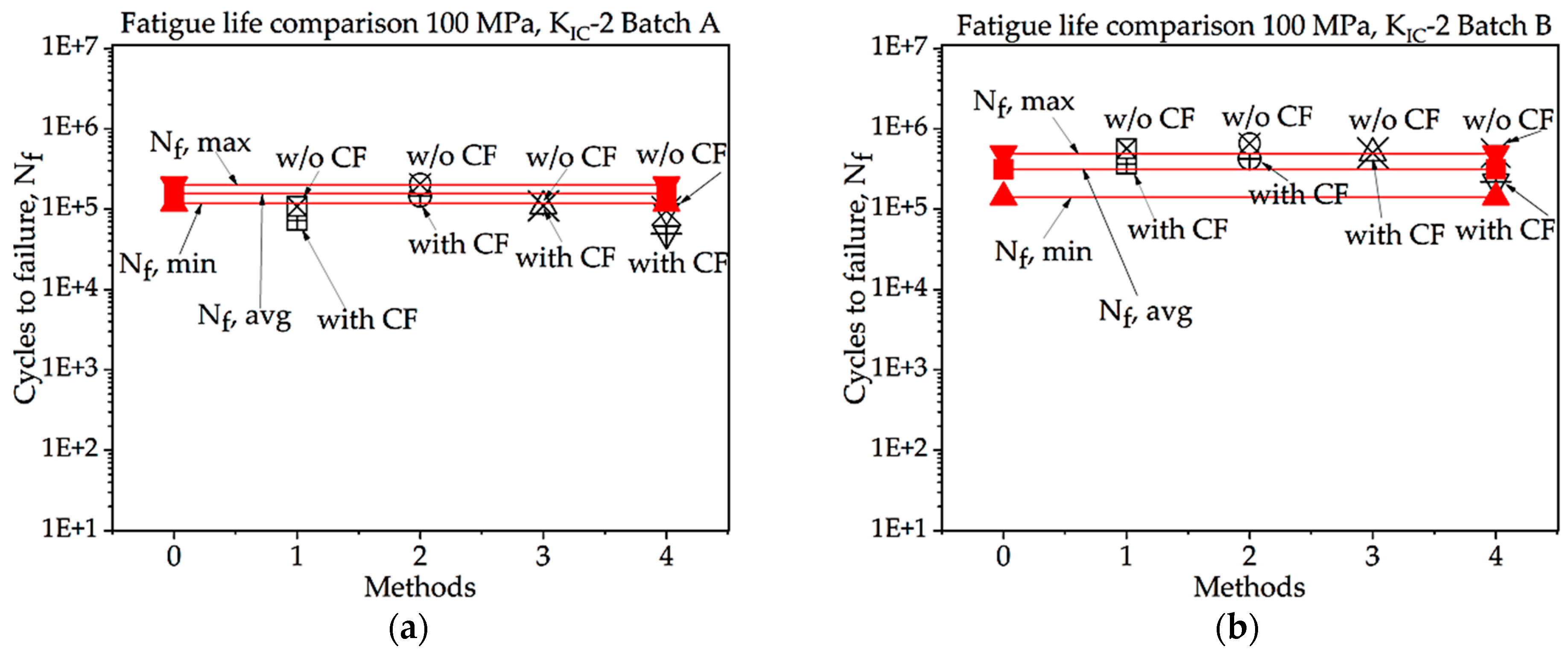
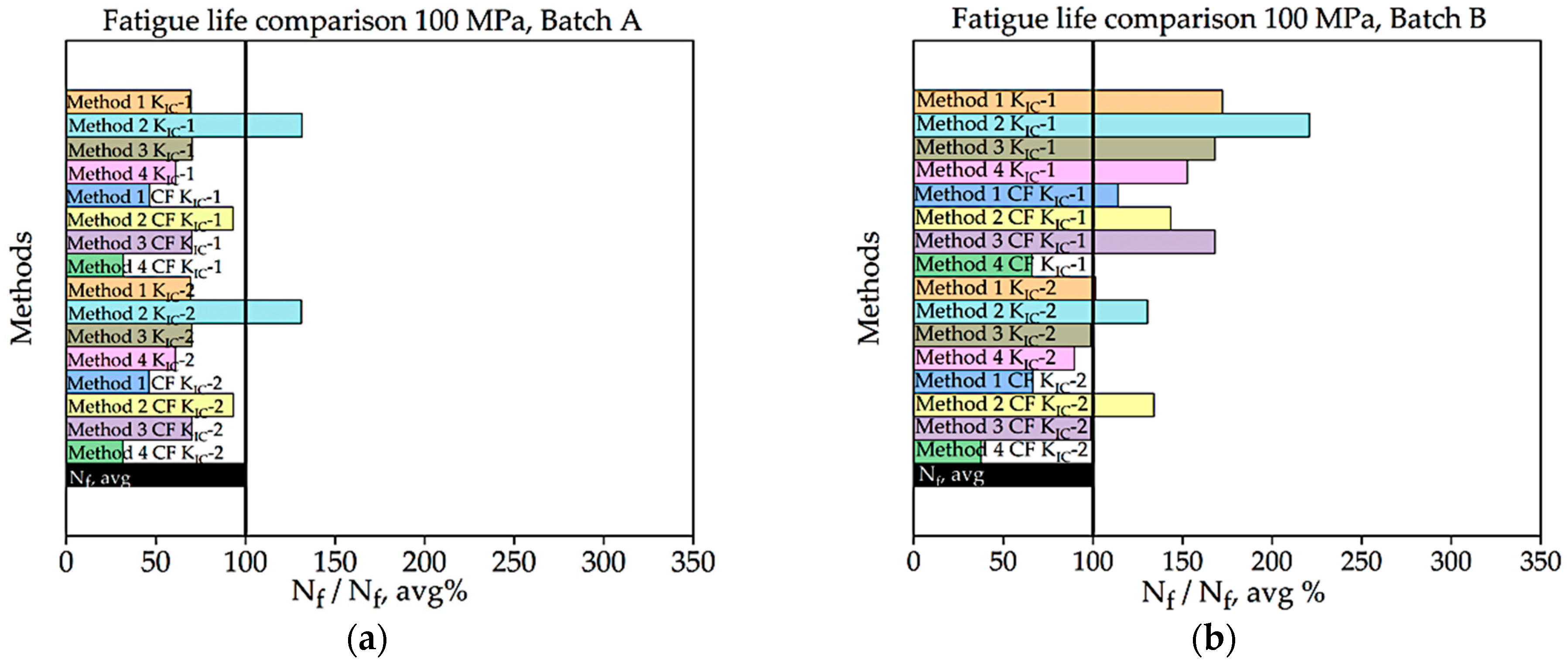
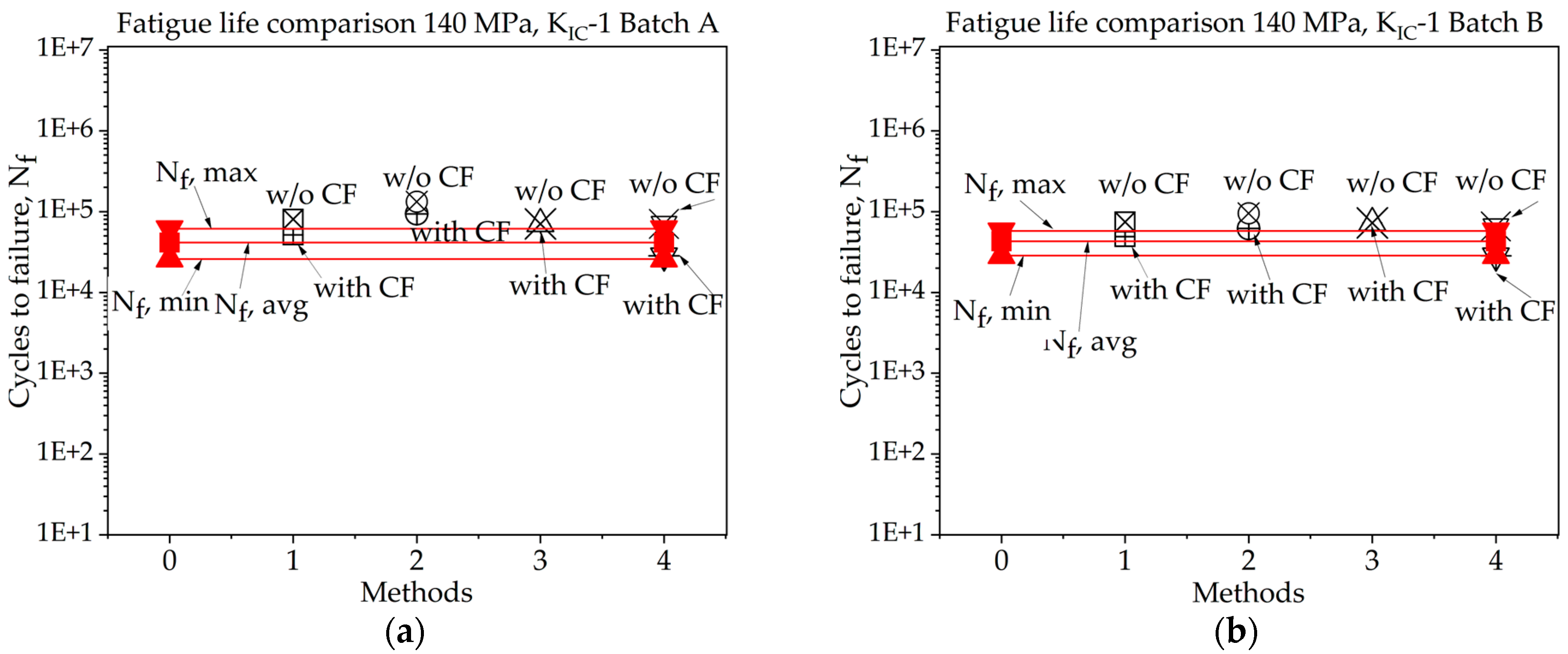
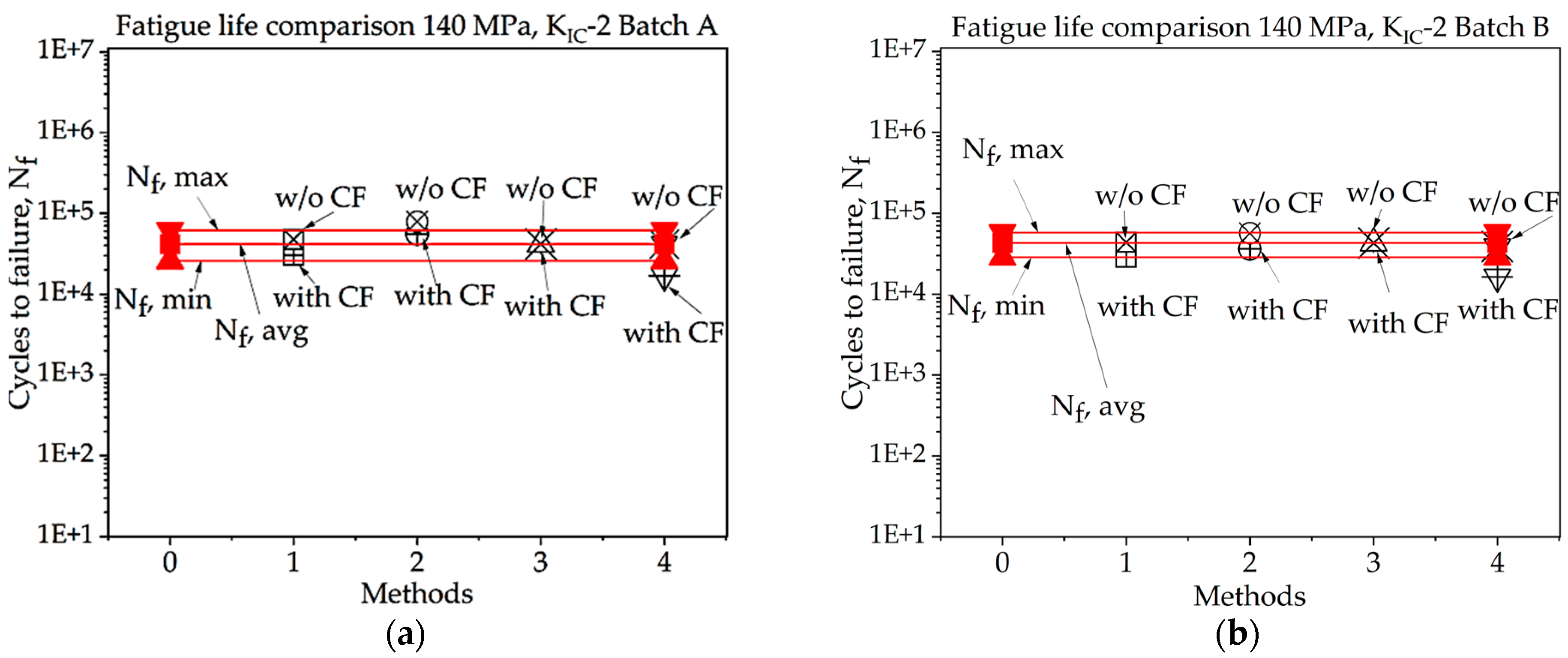
3.3. Fatigue Life Calculation
4. Conclusions
Author Contributions
Funding
Data Availability Statement
Acknowledgments
Conflicts of Interest
References
- Brennan, M.C.; Keist, J.S.; Palmer, T.A. Defects in metal additive manufacturing processes. J. Mater. Eng. Perform. 2021, 30, 4808–4818. [Google Scholar] [CrossRef]
- Sanaei, N.; Fatemi, A. Analysis of the effect of internal defects on fatigue performance of additive manufactured metals. Mater. Sci. Eng. A 2020, 785, 139385. [Google Scholar] [CrossRef]
- Madia, M.; Zerbst, U.; Werner, T. Estimation of the Kitagawa-Takahashi diagram by cyclic R curve analysis. Procedia Struct. Integr. 2022, 38, 309–316. [Google Scholar] [CrossRef]
- Pugno, N.; Ciavarella, M.; Cornetti, P.; Carpinteri, A. A generalized Paris’ law for fatigue crack growth. J. Mech. Phys. Solids 2006, 54, 1333–1349. [Google Scholar] [CrossRef]
- Awd, M.; Siddique, S.; Johannsen, J.; Emmelmann, C.; Walther, F. Very high-cycle fatigue properties and microstructural damage mechanisms of selective laser melted AlSi10Mg alloy. Int. J. Fatigue 2019, 124, 55–69. [Google Scholar] [CrossRef]
- Anderson, T.L.; Anderson, T.L. Fracture Mechanics; CRC Press: Boca Raton, FL, USA, 2005; ISBN 9780429125676. [Google Scholar]
- Kitagawa, H.; Takahashi, S. Applicability of fracture mechanics to very small cracks or the cracks in the early stage. Int. Conf. Mech. Behav. Biomater. 1976, 2, 627–631. [Google Scholar]
- El Haddad, M.H.; Smith, K.N.; Topper, T.H. Fatigue Crack Propagation of Short Cracks. J. Eng. Mater. Technol. 1979, 101, 42–46. [Google Scholar] [CrossRef]
- Pessard, E.; Lavialle, M.; Laheurte, P.; Didier, P.; Brochu, M. High-cycle fatigue behavior of a laser powder bed fusion additive manufactured Ti-6Al-4V titanium: Effect of pores and tested volume size. Int. J. Fatigue 2021, 149, 106206. [Google Scholar] [CrossRef]
- Sausto, F.; Carrion, P.E.; Shamsaei, N.; Beretta, S. Fatigue failure mechanisms for AlSi10Mg manufactured by L-PBF under axial and torsional loads: The role of defects and residual stresses. Int. J. Fatigue 2022, 162, 106903. [Google Scholar] [CrossRef]
- Garb, C.; Leitner, M.; Stauder, B.; Schnubel, D.; Grün, F. Application of modified Kitagawa-Takahashi diagram for fatigue strength assessment of cast Al-Si-Cu alloys. Int. J. Fatigue 2018, 111, 256–268. [Google Scholar] [CrossRef]
- ASTM E647-23a; Test Method for Measurement of Fatigue Crack Growth Rates. ASTM International: West Conshohocken, PA, USA, 2013.
- Murakami, Y. Effect of Hardness HV on Fatigue Limits of Materials Containing Defects, and Fatigue Limit Prediction Equations. Met. Fatigue 2002, 57–74. [Google Scholar] [CrossRef]
- Wu, S.C.; Song, Z.; Kang, G.Z.; Hu, Y.N.; Fu, Y.N. The Kitagawa-Takahashi fatigue diagram to hybrid welded AA7050 joints via synchrotron X-ray tomography. Int. J. Fatigue 2019, 125, 210–221. [Google Scholar] [CrossRef]
- Bartosiewicz, L.; Krause, A.R.; Sengupta, A.; Putatunda, S.K. Application of a new model for fatigue threshold in a structural steel weldment. Eng. Fract. Mech. 1993, 45, 463–477. [Google Scholar] [CrossRef]
- Zhang, C.; Gao, M.; Zeng, X. Effect of microstructural characteristics on high cycle fatigue properties of laser-arc hybrid welded AA6082 aluminum alloy. J. Mater. Process. Technol. 2016, 231, 479–487. [Google Scholar] [CrossRef]
- Murakami, Y. Effects of Small Defects and Nonmetallic Inclusions on the Fatigue Strength of Metals. JSME Int. J. Ser. 1 Solid Mech. Strength Mater. 1989, 32, 167–180. [Google Scholar] [CrossRef]
- Murakami, Y.; Fukuda, S.; Endo, T. Effect of Micro-hole on Fatigue Strength 1st Report, Effect of Micro-hole: Dia.: 40/50/80/100 & 200 μm) on the Fatigue Strength of 0.13% and 0.46% Carbon Steels. JSMET 1978, 44, 4003–4013. [Google Scholar] [CrossRef]
- Murakami, Y.; Endo, T. The effects of small defects on the fatigue strength of hard steels. Mater. Exp. Des. Fatigue 1981, 16, 431–440. [Google Scholar]
- Murakami, Y.; Endo, T. Effects of small defects on fatigue strength of metals. Int. J. Fatigue 1980, 2, 23–30. [Google Scholar] [CrossRef]
- Chen, X.; Hutchinson, J.W. Particle impact on metal substrates with application to foreign object damage to aircraft engines. J. Mech. Phys. Solids 2002, 50, 2669–2690. [Google Scholar] [CrossRef]
- Gerberich, W.W.; Davidson, D.L.; Kaczorowski, M. Experimental and theoretical strain distributions for stationary and growing cracks. J. Mech. Phys. Solids 1990, 38, 87–113. [Google Scholar] [CrossRef]
- Masuo, H.; Tanaka, Y.; Morokoshi, S.; Yagura, H.; Uchida, T.; Yamamoto, Y.; Murakami, Y. Influence of defects, surface roughness and HIP on the fatigue strength of Ti-6Al-4V manufactured by additive manufacturing. Int. J. Fatigue 2018, 117, 163–179. [Google Scholar] [CrossRef]
- Murakami, Y.; Kodama, S.; Konuma, S. Quantitative evaluation of effects of non-metallic inclusions on fatigue strength of high strength steels. I: Basic fatigue mechanism and evaluation of correlation between the fatigue fracture stress and the size and location of non-metallic inclusions. Int. J. Fatigue 1989, 11, 291–298. [Google Scholar] [CrossRef]
- Xu, Z.; Liu, A.; Wang, X.; Liu, B.; Guo, M. Fatigue limit prediction model and fatigue crack growth mechanism for selective laser melting Ti6Al4V samples with inherent defects. Int. J. Fatigue 2021, 143, 106008. [Google Scholar] [CrossRef]
- Rigon, D.; Meneghetti, G. An engineering estimation of fatigue thresholds from a microstructural size and Vickers hardness: Application to wrought and additively manufactured metals. Int. J. Fatigue 2020, 139, 105796. [Google Scholar] [CrossRef]
- Chapetti, M.D. A simple model to predict the very high cycle fatigue resistance of steels. Int. J. Fatigue 2011, 33, 833–841. [Google Scholar] [CrossRef]
- Schönbauer, B.M.; Mayer, H. Effect of small defects on the fatigue strength of martensitic stainless steels. Int. J. Fatigue 2019, 127, 362–375. [Google Scholar] [CrossRef]
- Yang, Z.G.; Zhang, J.M.; Li, S.X.; Li, G.Y.; Wang, Q.Y.; Hui, W.J.; Weng, Y.Q. On the critical inclusion size of high strength steels under ultra-high cycle fatigue. Mater. Sci. Eng. A 2006, 427, 167–174. [Google Scholar] [CrossRef]
- Suresh, S.; Ritchie, R.O. Propagation of short fatigue cracks. Int. Mater. Rev. 1984, 29, 445–475. [Google Scholar] [CrossRef]
- Benedetti, M.; Fontanari, V.; Bandini, M.; Zanini, F.; Carmignato, S. Low- and high-cycle fatigue resistance of Ti-6Al-4V ELI additively manufactured via selective laser melting: Mean stress and defect sensitivity. Int. J. Fatigue 2018, 107, 96–109. [Google Scholar] [CrossRef]
- Pang, J.C.; Li, S.X.; Wang, Z.G.; Zhang, Z.F. General relation between tensile strength and fatigue strength of metallic materials. Mater. Sci. Eng. A 2013, 564, 331–341. [Google Scholar] [CrossRef]
- ASTM E399-22; Standard Test Method for Linear-Elastic Plane-Strain Fracture Toughness of Metallic Materials. ASTM International: West Conshohocken, PA, USA, 2023.
- Petersen, R.C.; Lemons, J.E.; McCracken, M.S. Fracture toughness micromechanics by energy methods with a photocure fiber-reinforced composite. Polym. Compos. 2007, 28, 311–324. [Google Scholar] [CrossRef] [PubMed]
- Griffith, A.A., VI. The phenomena of rupture and flow in solids. Philos. Trans. R. Soc. Lond. Ser. A 1921, 221, 163–198. [Google Scholar] [CrossRef]
- Tada, H.; Paris, P.C.; Irwin, G.R. The Stress Analysis of Cracks Handbook, 3rd ed.; ASME Press: New York, NY, USA, 2000; ISBN 0791801535. [Google Scholar]
- Wei, R.P. Fracture Mechanics; Cambridge University Press: Cambridge, UK, 2012; ISBN 9780521194891. [Google Scholar]
- Krupp, U. Fatigue Crack Propagation in Metals and Alloys: Microstructural Aspects and Modelling Concepts; Wiley-VCH; John Wiley [distributor]: Weinheim, Germany; Chichester, UK, 2007; ISBN 1280921609. [Google Scholar]
- Petersen, R.C.; Lemons, J.E.; McCracken, M.S. Stress-Transfer Micromechanics for fiber length with a photocure vinyl ester composite. Polym. Compos. 2006, 27, 153–169. [Google Scholar] [CrossRef] [PubMed]
- Orowan, E. Fracture and strength of solids. Rep. Prog. Phys. 1949, 12, 185–232. [Google Scholar] [CrossRef]
- Callister, W.D. Materials Science and Engineering: An Introduction, 4th ed.; J. Wiley: New York, NY, USA, 1997; ISBN 0471134597. [Google Scholar]
- Bortz, S. Reliability of Ceramics for Heat Engine Applications. In Ceramics for High-Performance Applications III; Springer: Boston, MA, USA, 1983; pp. 445–473. [Google Scholar]
- Nezhadfar, P.D.; Thompson, S.; Saharan, A.; Phan, N.; Shamsaei, N. Structural integrity of additively manufactured aluminum alloys: Effects of build orientation on microstructure, porosity, and fatigue behavior. Addit. Manuf. 2021, 47, 102292. [Google Scholar] [CrossRef]
- Sundar. How to Calculate Fatigue Life? ExtruDeisgn.com [Online]. 2 February 2022. Available online: https://extrudesign.com/how-to-calculate-fatigue-life/ (accessed on 21 August 2023).
- Radhakrishnan, V.M. Quantifying the parameters in fatigue crack propagation. Eng. Fract. Mech. 1980, 13, 129–141. [Google Scholar] [CrossRef]
- Niccolls, E.H. A correlation for fatigue crack growth rate. Scr. Metall. 1976, 10, 295–298. [Google Scholar] [CrossRef]
- Cavallini, M.; Iacoviello, F. Fatigue models for Al alloys. Int. J. Fatigue 1991, 13, 442–446. [Google Scholar] [CrossRef]
- Materials Park: ASM International. ASM Handbook: Fatigue and Fracture, 1985–1988; ASM International: Novelty, OH, USA, 1988; ISBN 978-0-87170-385-9. [Google Scholar]
- Materials Park: ASM International. Metals Handbook, 1985; ASM International: Novelty, OH, USA, 1985; ISBN 0-87170-654-7. [Google Scholar]
- Ho, C.Y.; Holt, J.M.; Mindlin, H. Structural Alloys Handbook: 1996 Edition; Incorporating Supplements Throught 1995; Cindas/Purdue Univ: West Lafayette, IN, USA, 1997. [Google Scholar]
- Properties and Selection: Nonferrous Alloys and Special-Purpose Materials; ASM International: Novelty, OH, USA, 1990; ISBN 978-1-62708-162-7.
- Biswal, R.; Zhang, X.; Syed, A.K.; Awd, M.; Ding, J.; Walther, F.; Williams, S. Criticality of porosity defects on the fatigue performance of wire + arc additive manufactured titanium alloy. Int. J. Fatigue 2019, 122, 208–217. [Google Scholar] [CrossRef]
- Yu, M.; Duquesnay, D.; Topper, T. Notch fatigue behaviour of SAE1045 steel. Int. J. Fatigue 1988, 10, 109–116. [Google Scholar] [CrossRef]
- Beretta, S.; Romano, S. A comparison of fatigue strength sensitivity to defects for materials manufactured by AM or traditional processes. Int. J. Fatigue 2017, 94, 178–191. [Google Scholar] [CrossRef]
- Atzori, B.; Lazzarin, P.; Meneghetti, G. Fracture mechanics and notch sensitivity. Fatigue Fract. Eng. Mater. Struct. 2003, 26, 257–267. [Google Scholar] [CrossRef]
- Atzori, B.; Lazzarin, P.; Meneghetti, G. A unified treatment of the mode I fatigue limit of components containing notches or defects. Int. J. Fract. 2005, 133, 61–87. [Google Scholar] [CrossRef]
- Kasperovich, G.; Hausmann, J. Improvement of fatigue resistance and ductility of TiAl6V4 processed by selective laser melting. J. Mater. Process. Technol. 2015, 220, 202–214. [Google Scholar] [CrossRef]
- Wolfenden, A.; Du Quesnay, D.L.; Yu, M.T.; Topper, T.H. An Analysis of Notch-Size Effects at the Fatigue Limit. J. Test. Eval. 1988, 16, 375. [Google Scholar] [CrossRef]


| Batch | Loading Condition | Best Method | Error Percentage |
|---|---|---|---|
| A | 120 | 1st with CF using KIC-1 | 5.8% |
| A | 100 | 2nd with CF using KIC-1 and 2 | 6.66% |
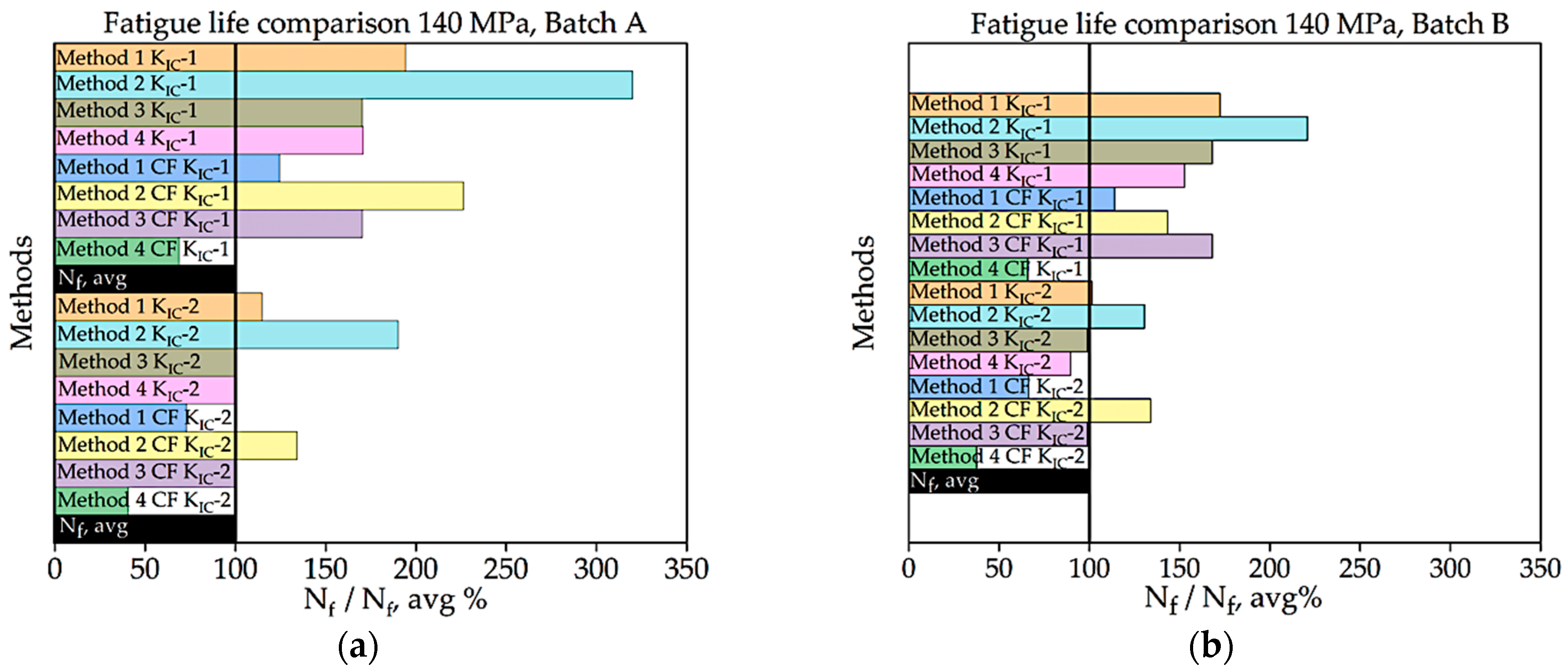
| A | 140 | 3rd and 4th without CF using KIC-2 | 0.5% |
| B | 120 | 1st with CF using KIC-1 | 0.29% |
| B | 100 | 1st without CF using KIC-1 | 4.3% |
| B | 140 | 1st and 3rd without CF using KIC-2 | 1% |
| Stress | 100 MPa | 120 MPa | 140 MPa | ||||||||||
|---|---|---|---|---|---|---|---|---|---|---|---|---|---|
| KIC Method | KIC-1 | KIC-2 | KIC-1 | KIC-2 | KIC-1 | KIC-2 | |||||||
| batch A | Nf/Nf,avg% | Error% | Nf/Nf,avg% | Error% | Nf/Nf,avg% | Error% | Nf/Nf,avg% | Error% | Nf/Nf,avg% | Error% | Nf/Nf,avg% | Error% | |
| Method 1 | 135% | −35% | 79% | 21% | 70% | 30% | 69% | 31% | 194% | −94% | 115% | −15% | |
| Method 2 | 282% | −182% | 167% | −67% | 132% | −32% | 131% | −31% | 320% | −220% | 190% | −90% | |
| Method 3 | 151% | −51% | 89% | 11% | 70% | 30% | 70% | 30% | 170% | −70% | 100% | 0% | |
| Method 4 | 119% | −19% | 69% | 31% | 61% | 39% | 61% | 39% | 171% | −71% | 101% | −1% | |
| Method 1 CF | 94% | 6% | 54% | 46% | 47% | 53% | 46% | 54% | 125% | −25% | 73% | 27% | |
| Method 2 CF | 200% | −100% | 118% | −18% | 93% | 7% | 93% | 7% | 226% | −126% | 134% | −34% | |
| Method 4 CF | 62% | 38% | 35% | 65% | 32% | 68% | 32% | 68% | 69% | 31% | 41% | 59% | |
| batch B | Method 1 | 188% | −88% | 155% | −55% | 96% | 4% | 181% | −81% | 173% | −73% | 102% | −2% |
| Method 2 | 226% | −126% | 185% | −85% | 110% | −10% | 209% | −109% | 221% | −121% | 131% | −31% | |
| Method 3 | 172% | −72% | 141% | −41% | 84% | 16% | 159% | −59% | 168% | −68% | 99% | 1% | |
| Method 4 | 167% | −67% | 136% | −36% | 84% | 16% | 160% | −60% | 153% | −53% | 90% | 10% | |
| Method 1 CF | 121% | −21% | 100% | 0% | 61% | 39% | 116% | −16% | 114% | −14% | 66% | 34% | |
| Method 2 CF | 146% | −46% | 120% | −20% | 72% | 28% | 136% | −36% | 143% | −43% | 84% | 16% | |
| Method 4 CF | 72% | 28% | 59% | 41% | 37% | 63% | 70% | 30% | 66% | 34% | 38% | 62% | |
Disclaimer/Publisher’s Note: The statements, opinions and data contained in all publications are solely those of the individual author(s) and contributor(s) and not of MDPI and/or the editor(s). MDPI and/or the editor(s) disclaim responsibility for any injury to people or property resulting from any ideas, methods, instructions or products referred to in the content. |
© 2023 by the authors. Licensee MDPI, Basel, Switzerland. This article is an open access article distributed under the terms and conditions of the Creative Commons Attribution (CC BY) license (https://creativecommons.org/licenses/by/4.0/).
Share and Cite
Nur, M.I.; Soni, M.; Awd, M.; Walther, F. Comparison of Various Intrinsic Defect Criteria to Plot Kitagawa–Takahashi Diagrams in Additively Manufactured AlSi10Mg. Materials 2023, 16, 6334. https://doi.org/10.3390/ma16186334
Nur MI, Soni M, Awd M, Walther F. Comparison of Various Intrinsic Defect Criteria to Plot Kitagawa–Takahashi Diagrams in Additively Manufactured AlSi10Mg. Materials. 2023; 16(18):6334. https://doi.org/10.3390/ma16186334
Chicago/Turabian StyleNur, Mohammed Intishar, Meetkumar Soni, Mustafa Awd, and Frank Walther. 2023. "Comparison of Various Intrinsic Defect Criteria to Plot Kitagawa–Takahashi Diagrams in Additively Manufactured AlSi10Mg" Materials 16, no. 18: 6334. https://doi.org/10.3390/ma16186334