
Signal-Decay Based Approach for Visualization of Buried Defects in 3-D Printed Ceramic Components Imaged with Help of Optical Coherence Tomography

 ,
,  , and
, and
Abstract
:1. Introduction
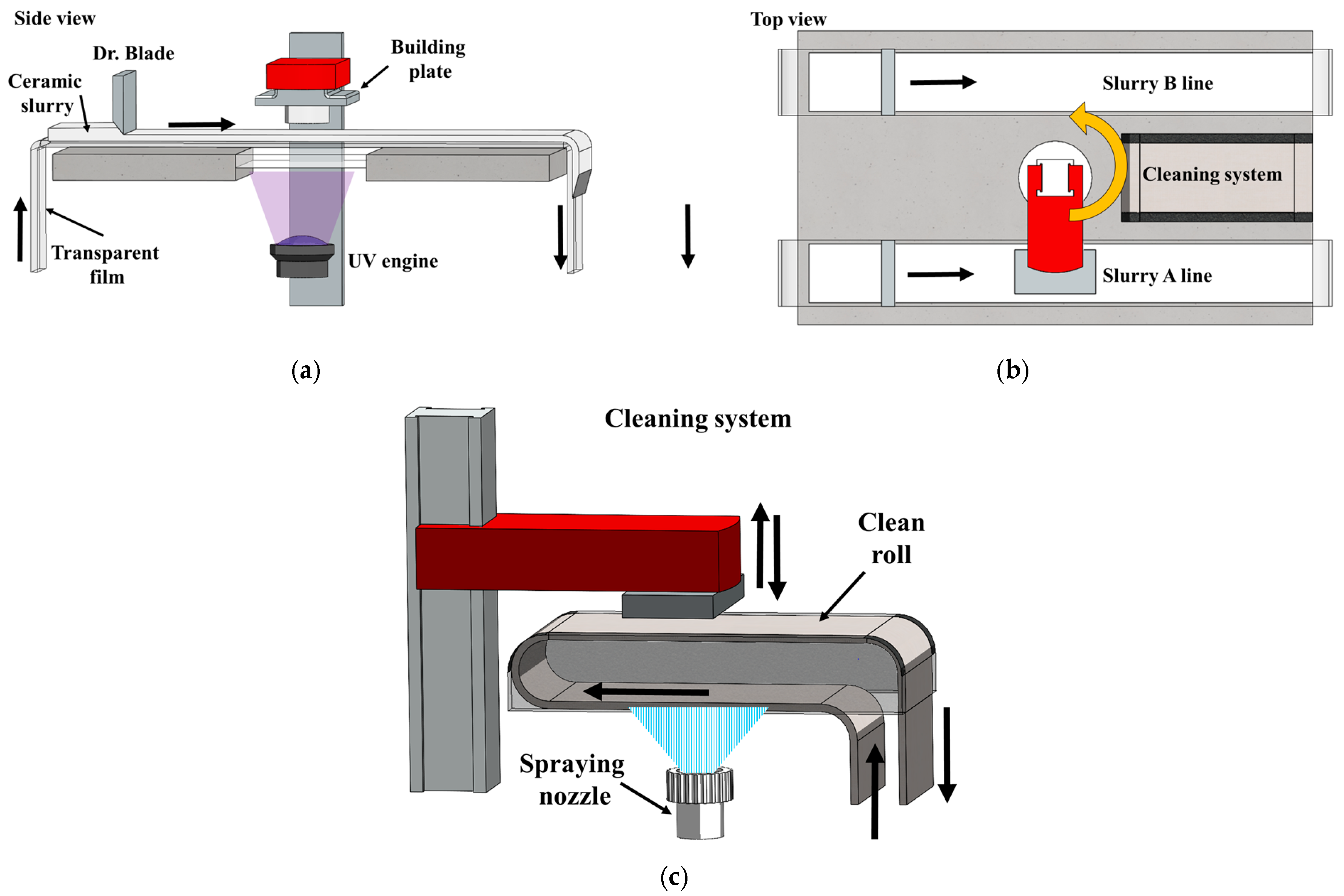
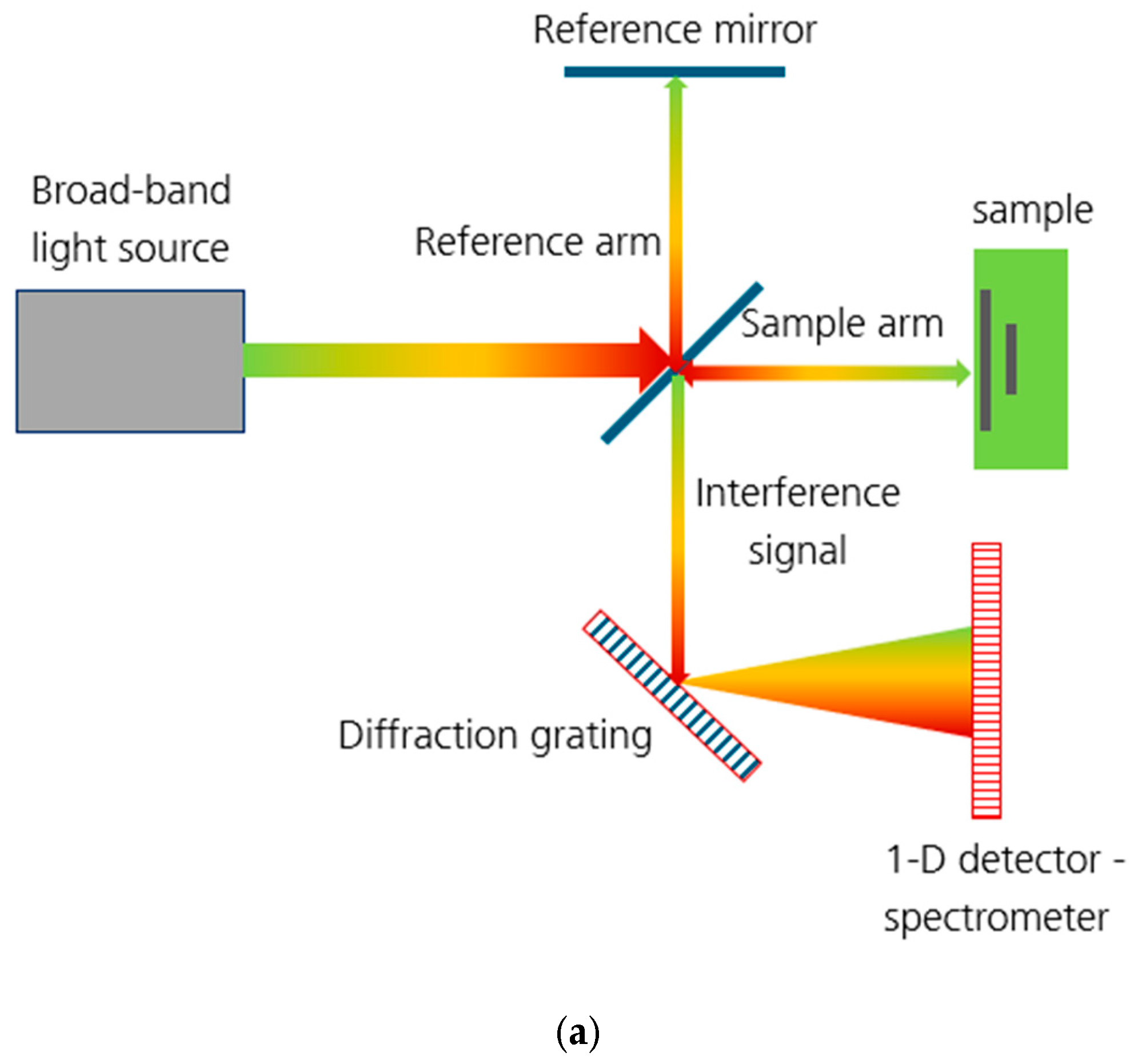
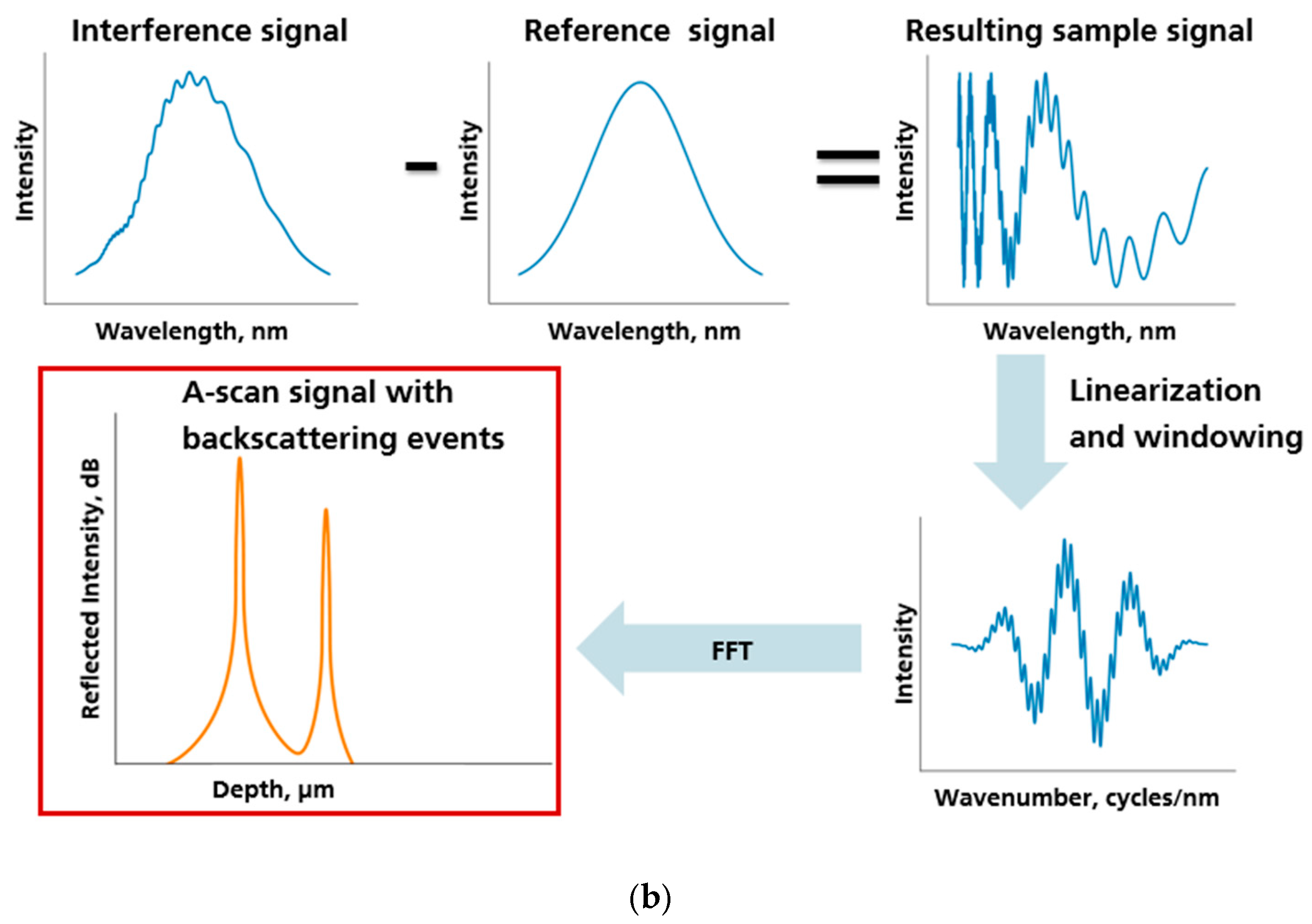
2. Materials and Methods
3. Results and Analysis
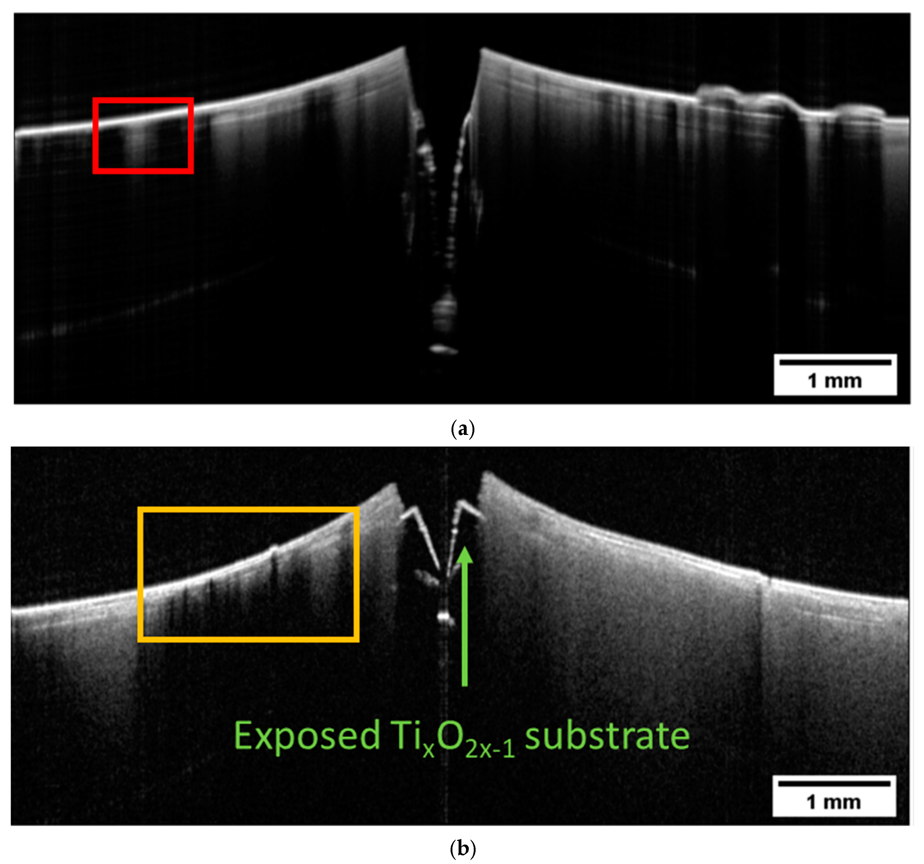
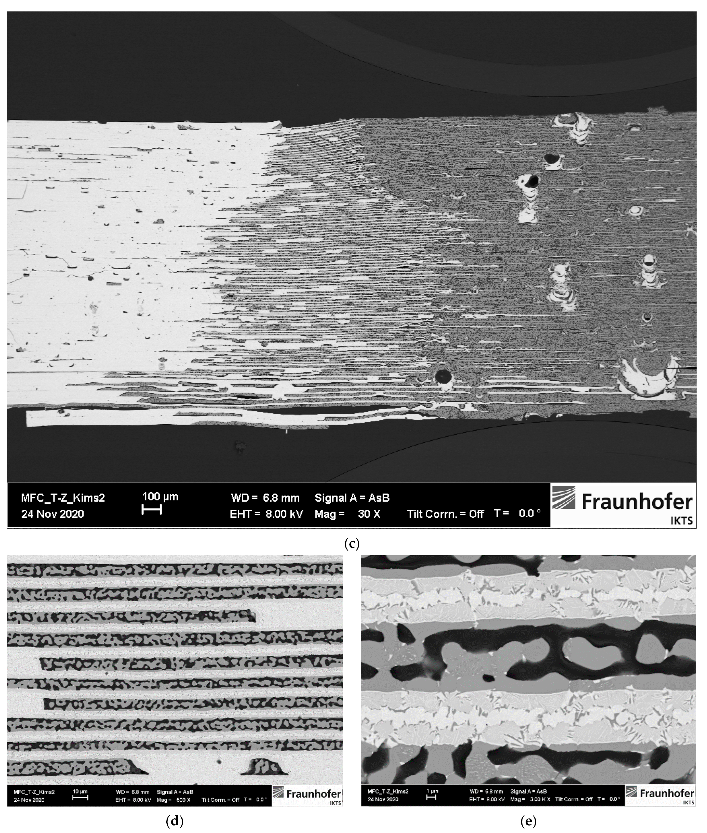
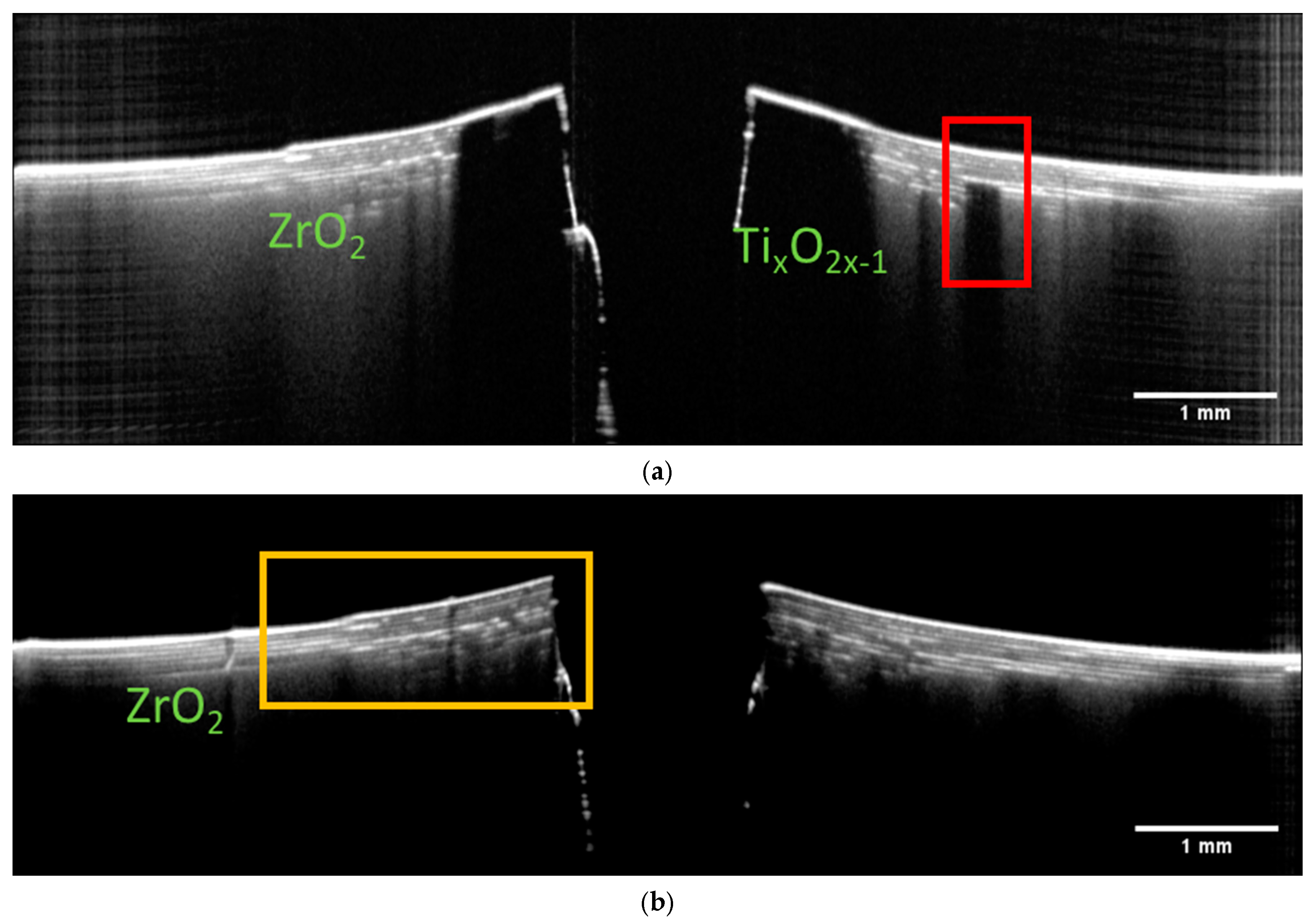
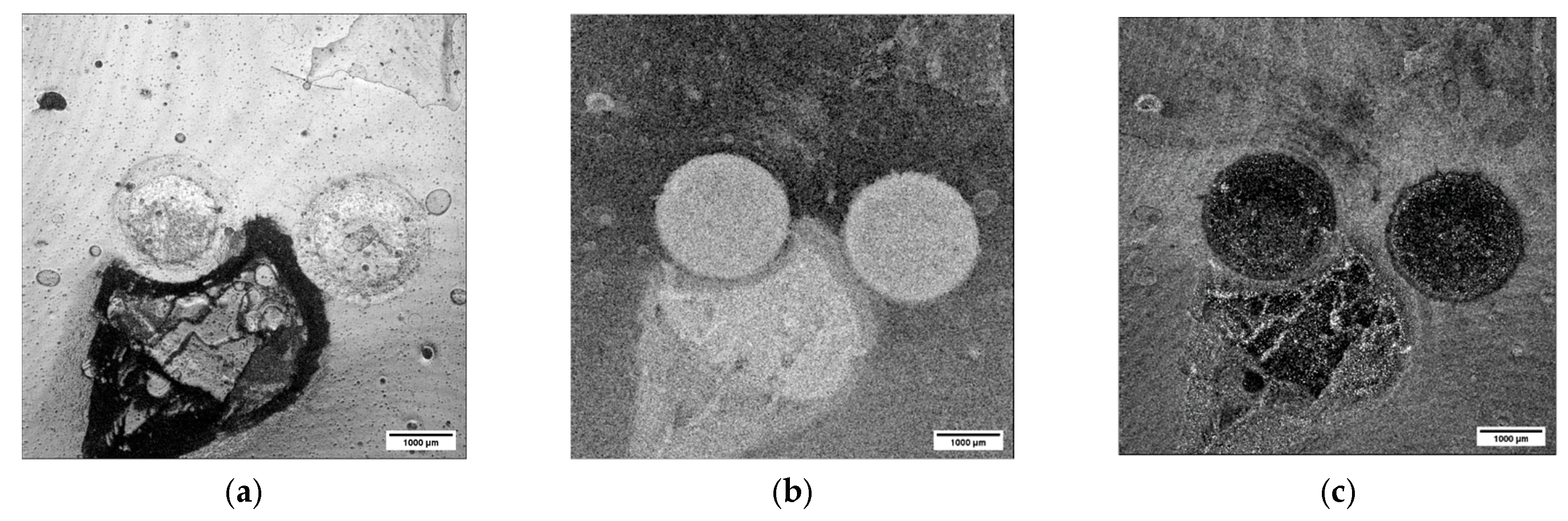
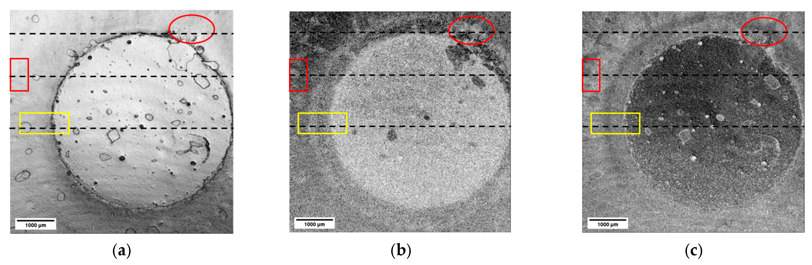
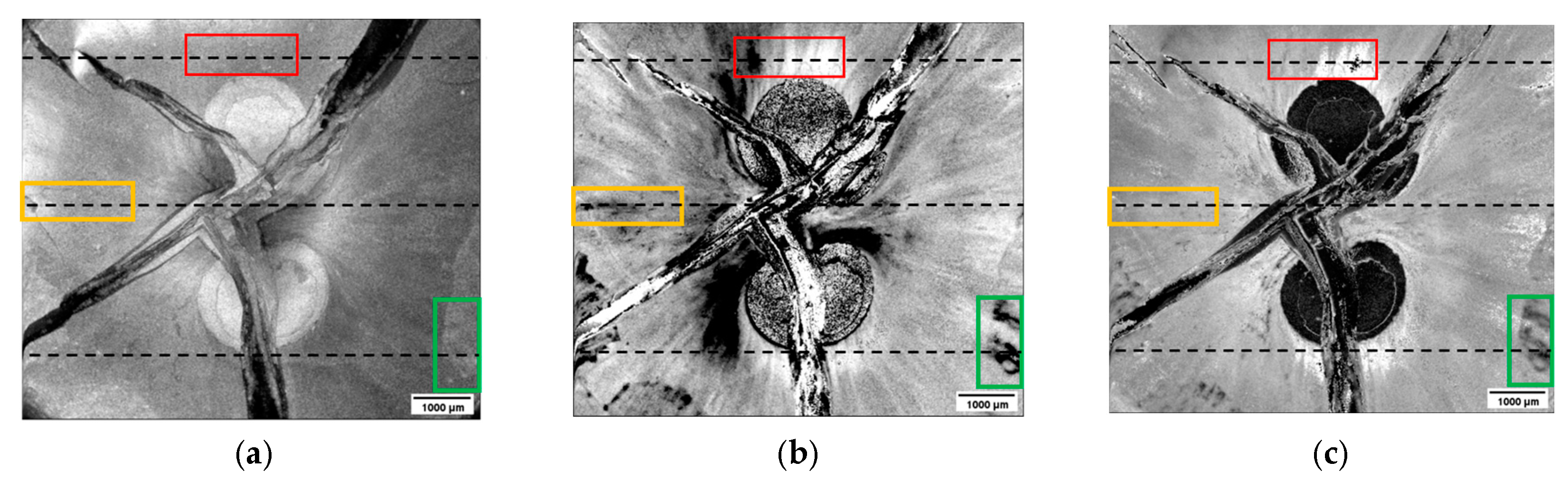
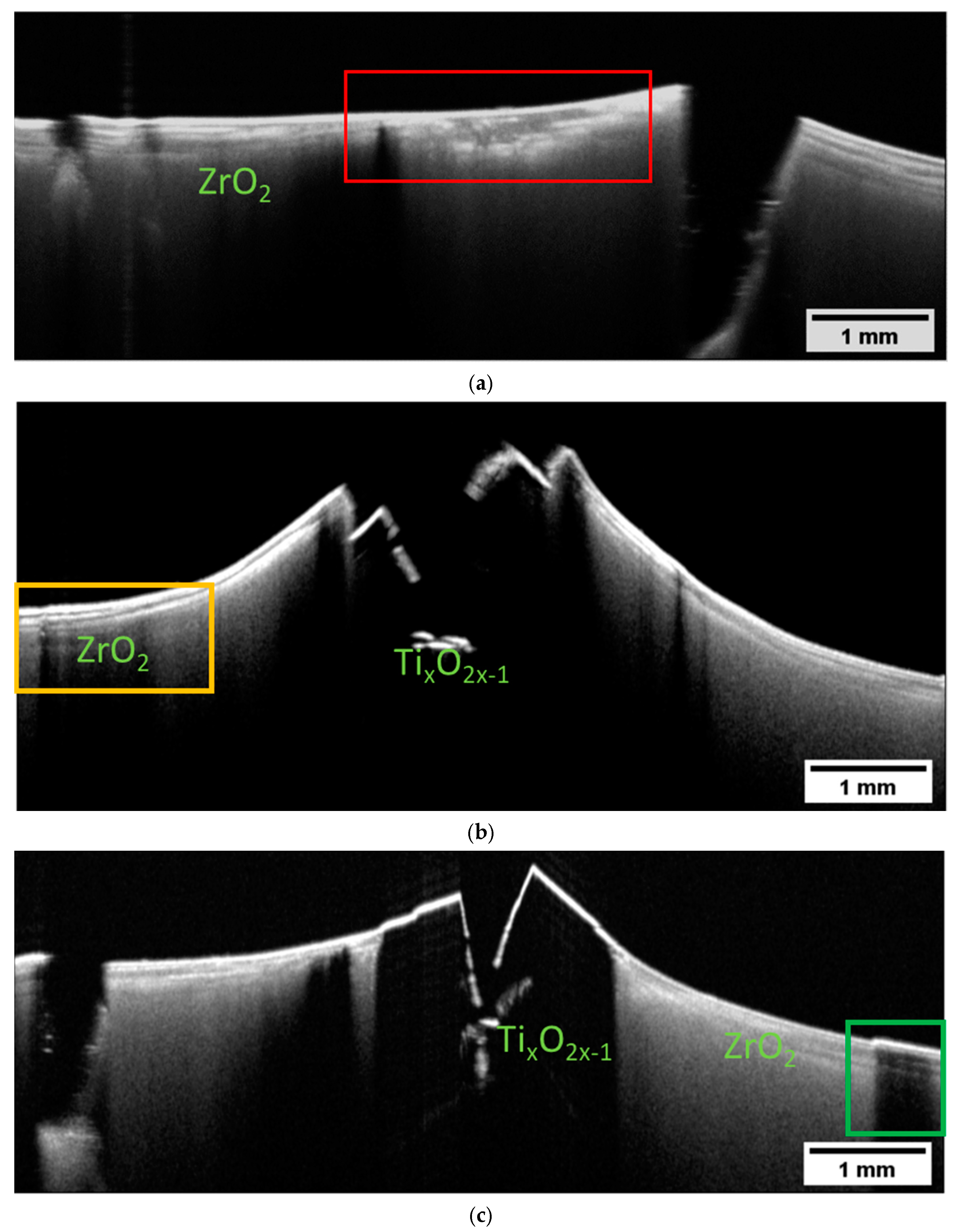
3.1. Qualitative Analysis at B-Scans Level
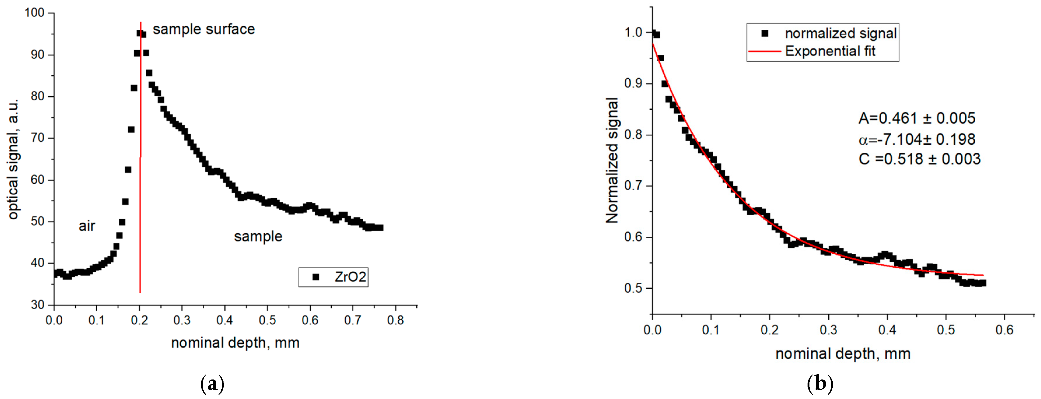
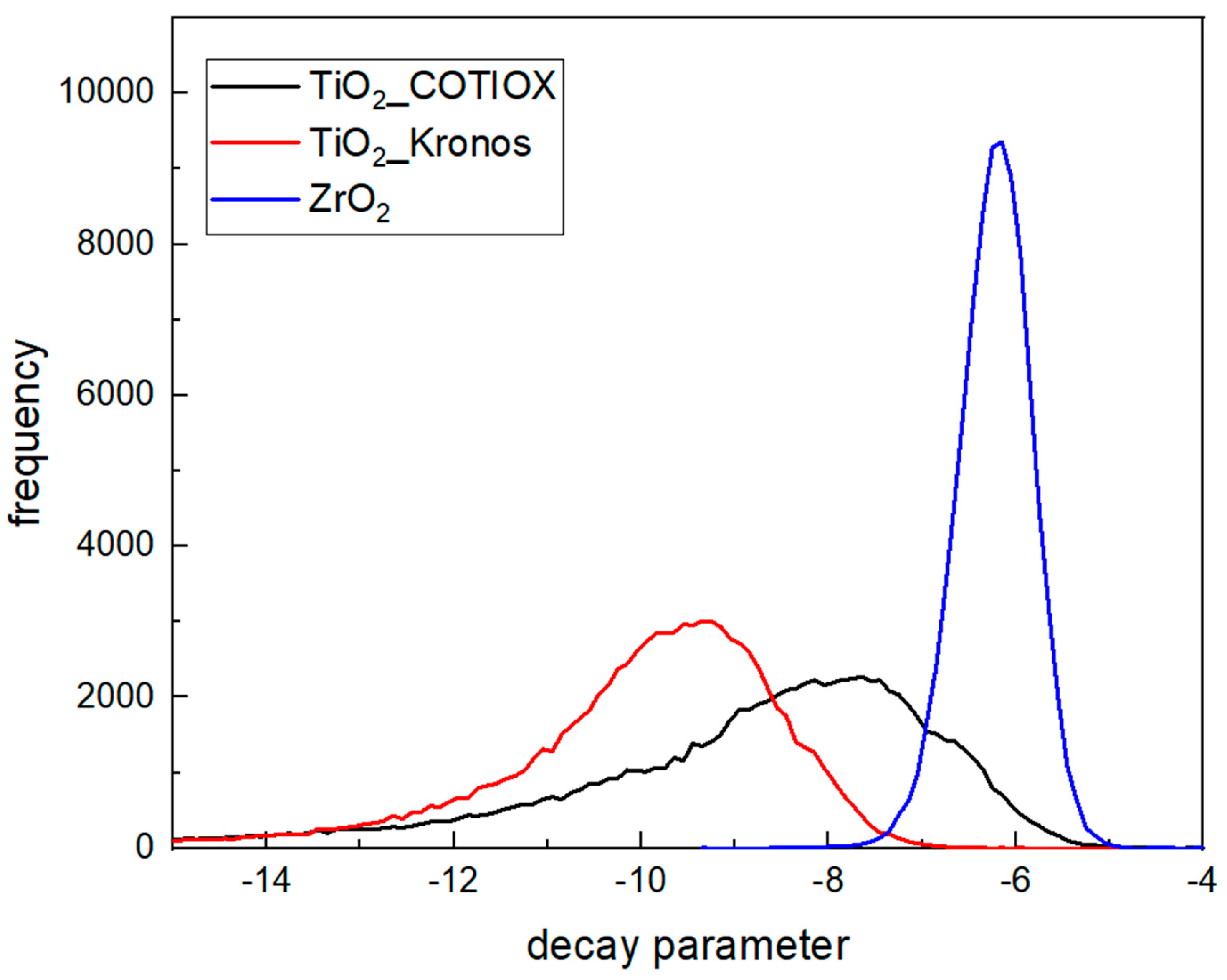
3.2. Data Analysis at A-Scan Level
4. Summary and Outlook
Author Contributions
Funding
Informed Consent Statement
Data Availability Statement
Acknowledgments
Conflicts of Interest
References
- Otitoju, T.A.; Okoye, P.U.; Chen, G.; Li, Y.; Okoye, M.O.; Li, S. Advanced ceramic components: Materials, Fabrication, and Application. J. Ind. Eng. Chem. 2020, 85, 34. [Google Scholar] [CrossRef]
- Marcus, H.L.; Beaman, J.J.; Barlow, J.W.; Bourell, D.L. Solid freeform fabrication-powder processing. Am. Ceram. Soc. Bull. 1990, 69, 1030. [Google Scholar]
- Sachs, E.; Cima, M.; Cornie, J. Three dimensional printing: Rapid tooling and prototypes directly from CAD model. CIRP Ann. Manuf. Technol. 1990, 39, 201. [Google Scholar] [CrossRef]
- Pelz, J.S.; Ku, N.; Meyers, M.A.; Vargas-Gonzalez, L.R. Additive manufacturing of structural ceramics: A historical perspective. J. Mater. Res. Technol. 2021, 15, 670. [Google Scholar] [CrossRef]
- Griffith, M.L.; Halloran, J.W. Freeform fabrication of ceramics via stereolithography. J. Am. Ceram. Soc. 1996, 79, 2601. [Google Scholar] [CrossRef] [Green Version]
- Subramanian, K.; Vail, N.; Barlow, J.; Marcus, H. Selective laser sintering of alumina with polymer binders. Rapid Prototype J. 1995, 1, 24. [Google Scholar] [CrossRef]
- Blazdell, P.F.; Evans, G.J.R.; Edirisinghe, M.J.; Shaw, P.; Binstead, M.J. The computer aided manufacture of ceramics using multilayer jet printing. J. Matter Sci. Lett. 1995, 14, 1562. [Google Scholar] [CrossRef]
- Feygin, M.; Hsieh, B. Laminated object manufacturing: A simpler process. In Proceedings of the 2nd Solid Freedom Fabrication Symposium, Austin, TX, USA, 12–14 August 1991; p. 123. [Google Scholar]
- Agarwala, M.K.; Bandyopadhyay, A.; van Weeren, R.; Safari, A.; Danforth, S.C.; Langarna, N.A.; Jamalabad, V.R.; Whalen, P.J. FDC, rapid fabrication of structural components. Am. Ceram. Soc. Bull. 1996, 75, 62. [Google Scholar]
- Tompkins, J.V.; Laabi, R.; Birmingham, B.R.; Marcus, H.L. Advances in selective area laser deposition of silicon carbide. In Proceedings of the 1994 International Solid Freeform Fabrication Symposium, Austin, TX, USA, 8–10 August 1994; p. 412. [Google Scholar]
- Chen, Z.; Li, Z.; Li, J.; Liu, C.; Lao, C.; Fu, Y.; Liu, C. 3D printing of ceramics: A review. J. Eur. Ceram. Soc. 2019, 39, 661. [Google Scholar] [CrossRef]
- Lakhdar, Y.; Tuck, C.; Binner, J.; Terry, A.; Goodridge, R. Additive manufacturing of advanced ceramic materials. Prog. Mater. Sci. 2021, 116, 100736. [Google Scholar] [CrossRef]
- Allen, A.J.; Levin, I.; Witt, S.E. Materials research and measurement needs for ceramics additive manufacturing. J. Am. Ceram. Soc. 2020, 103, 6055. [Google Scholar] [CrossRef] [PubMed]
- Schwarzer-Fischer, E.; Günther, A.; Roszeitis, S.; Moritz, T. Combining Zirconia and Titanium Suboxides by Vat Photopolymerization. Materials 2021, 14, 2394. [Google Scholar] [CrossRef] [PubMed]
- Kim, J.; Gal, C.W.; Choi, Y.-J.; Park, H.; Yoon, S.-Y.; Yun, H. Effect of non-reactive diluent on defect-free debinding process of 3-d printed ceramics. Addit. Manuf. 2023, 67, 103475. [Google Scholar] [CrossRef]
- Zhang, S.; Sutejo, I.A.; Kim, J.; Choi, Y.-J.; Gal, C.W.; Yun, H. Fabrication of complex three-dimentional structures of mica through digital light processing-based additive manufacturing. Ceramics 2022, 5, 562. [Google Scholar] [CrossRef]
- Kim, H.; Lin, Y.; Bill Tseng, T.-L. A review on quality control in additive manufacturing. Rapid Prototyp. J. 2018, 24, 645. [Google Scholar] [CrossRef] [Green Version]
- Lee, J.; Park, H.J.; Chai, S.; Kim, G.R.; Yong, H.; Bae, S.J. Review on quality control methods in metal additive manufacturing. Appl. Sci. 2021, 11, 1966. [Google Scholar] [CrossRef]
- Yoo, S.Y.; Kim, S.-K.; Heo, S.-J.; Koak, J.-Y.; Kim, J.-G. Dimensional accuracy of dental models for three unit prostheses fabricated by various 3D printing. Materials 2021, 14, 1550. [Google Scholar] [CrossRef]
- Msallem, B.; Sharma, N.; Cao, S.; Halbeisen, F.S.; Zeilhofer, H.-F.; Thieringer, F.M. Evaluation of the dimensional accuracy of 3-D-printed anatomical mandibular models using FFF, SLA, SLS MJ, and BJ printing technology. J. Clin. Med. 2020, 9, 817. [Google Scholar] [CrossRef] [PubMed] [Green Version]
- Opitz, J.; Porstmann, V.; Schreiber, L.; Schmalfuß, T.; Lehmann, A.; Naumann, S.; Schallert, R.; Rößler, S.; Wiesmann, H.P.; Kruppke, B.; et al. Optical Coherence Tomography as Monitoring Technology for the Additive Manufacturing of Future Biomedical Parts. In Handbook of Nondestructive Evaluation 4.0.; Meyendorf, N., Ida, N., Singh, R., Vrana, J., Eds.; Springer: Cham, Switzerland, 2021. [Google Scholar] [CrossRef]
- Wunderlich, C.; Bendjus, B.; Kopycinska-Müller, M. NDE in Additive Manufacturing of Ceramic Components. In Handbook of Nondestructive Evaluation 4.0.; Meyendorf, N., Ida, N., Singh, R., Vrana, J., Eds.; Springer: Cham, Switzerland, 2021. [Google Scholar] [CrossRef]
- Zorin, I.; Brouczek, D.; Geier, S.; Nohut, S.; Eichelseder, J.; Huss, G.; Schwentenwein, M.; Heise, B. Mid-Infrared optical coherence tomography as a method for inspection and quality assurance in ceramics additive manufacturing. Open Ceram. 2022, 12, 100311. [Google Scholar] [CrossRef]
- Huang, D.; Swanson, E.A.; Lin, C.P.; Schuman, J.S.; Stinson, W.G.; Chang, W.; Hee, M.R.; Flotte, T.; Gregory, K.; Puliafito, C.A.; et al. Optical Coherence Tomography. Science 1991, 254, 1178. [Google Scholar] [CrossRef] [Green Version]
- Fercher, A.F.; Drexler, W.; Hitzenberger, C.K.; Lasser, T. Optical Coherence tomography—Principles and applications. Rep. Prog. Phys. 2003, 66, 239. [Google Scholar] [CrossRef]
- Schmitt, J.M. Optical coherence Tomography (OCT): A review. IEEE J. Sel. Top. Quantum Electron. 1999, 5, 1205. [Google Scholar] [CrossRef] [Green Version]
- Fercher, A.F.; Hitzenberger, C.K.; Kamp, G.; El-Zaiat, S.Y. Measurements of intraocular distances by backscattering spectral interferometry. Opt. Commun. 1995, 117, 43. [Google Scholar] [CrossRef]
- Aumann, S.; Donner, S.; Fischer, J.; Müller, F. Optical Coherence Tomography (OCT): Principle and technical realization. In High Resolution Imaging in Microscopy and Ophthalmology; Bille, J.F., Ed.; University Heidelberg: Heidelberg, Germany; Springer: Berlin/Heidelberg, Germany, 2019. [Google Scholar]
- de Boer, J.F.; Cense, B.; Park, B.H.; Pierce, M.C.; Tearney, G.J.; Bouma, B.E. Improved signal-to-noice ratio in spectral-domain compared with time-domain optical coherence tomography. Opt. Lett. 2003, 28, 2067. [Google Scholar] [CrossRef] [PubMed]
- Ali, M.; Parlapali, R. Signal Processing Overview of Optical Coherence Tomography Systems for Medical Imaging; White Paper, SPRABB9-June 2010; Texas Instruments Incorporated: Dallas, TX, USA, 2010. [Google Scholar]
- Ding, Z.; Ren, H.; Zhao, Y.; Nelson, J.S.; Chen, Z. High resolution Optical coherence Tomography over a large depth range with an Axion lens. Opt. Lett. 2002, 27, 243. [Google Scholar] [CrossRef]
- Tomlins, P.H.; Wang, R.K. Theory, developments and applications of Optical coherence Tomography. J. Phys. D Appl. Phys. 2005, 38, 1219. [Google Scholar] [CrossRef]
- Hayfield, P.C.S. Development of a New Material—Monolithic Ti4O7 Ebonex®Ceramic; MFIS Ltd.: London, UK, 2002; ISBN 0-85404-984-3. [Google Scholar]
- Zhang, X.; Liu, Y.; Ye, J. Fabrication and characterization of Magneli phase Ti4O7 nanoparticles. Micro Nano Lett. 2013, 8, 251. [Google Scholar] [CrossRef]
- Ran, A.R.; Tham, C.C.; Chan, P.P.; Cheng, C.-Y.; Tham, Y.C.; Rim, T.H.; Cheung, C.Y. Deep learning in glaucoma with optical coherence tomography: A review. Eye 2021, 35, 188. [Google Scholar] [CrossRef]
- Faber, D.J.; van der Meer, F.J.; Aalders, M.C.G.; Van Leeuwen, T.G. Quantitative measurements of attenuation coefficients of weakly scattering media using optical coherence tomography. Opt. Express 2004, 12, 4353. [Google Scholar] [CrossRef] [Green Version]
- Levitz, D.; Thrane, L.; Frosz, M.H.; Andersen, P.E.; Andersen, C.B.; Valanciunaite, J.; Swartling, J.; Andersson-Engels, S.; Hansen, P. Determination of optical scattering properties of highly scattering media in optical coherence tomography. Opt. Express 2004, 12, 249. [Google Scholar] [CrossRef] [Green Version]
- Yashin, K.S.; Kiseleva, E.B.; Moiseev, A.A.; Kuznetsov, S.S.; Timofeeva, L.B.; Pavlova, N.P.; Gelikonov, G.V.; Medyanik, I.A.; Kravets, L.Y.; Zagaynova, E.V.; et al. Quantitative nontumorous and tumorous human brain tissue assessment using microstructural co- and cross-polarized optical coherence tomography. Sci. Rep. 2019, 9, 2024. [Google Scholar] [CrossRef] [PubMed] [Green Version]
- Foo, K.Y.; Chin, L.; Zilkens, R.; Lakhiani, D.D.; Fang, Q.; Sanderson, R.; Dessauvagie, B.F.; Latham, B.; McLaren, S.; Saunders, C.M.; et al. Three-dimensional mapping of the attenuation coefficient in optical coherence tomography to enhance breast tissue microarchitecture contrast. J. Biophotonics 2020, 13, e201960201. [Google Scholar] [CrossRef] [PubMed]
- Yuan, W.; Kut, C.; Liang, W.; Li, X. Robust and fast characterization of OCT-based optical attenuation using a novel frequency-domain algorithm for brain cancer detection. Sci. Rep. 2017, 7, 44909. [Google Scholar] [CrossRef] [PubMed] [Green Version]
- Toyokura, S. Contactless mapping of ceramic green density using optical coherence tomography. Open Ceram. 2021, 5, 100061. [Google Scholar] [CrossRef]


| Green | Sintered | |
|---|---|---|
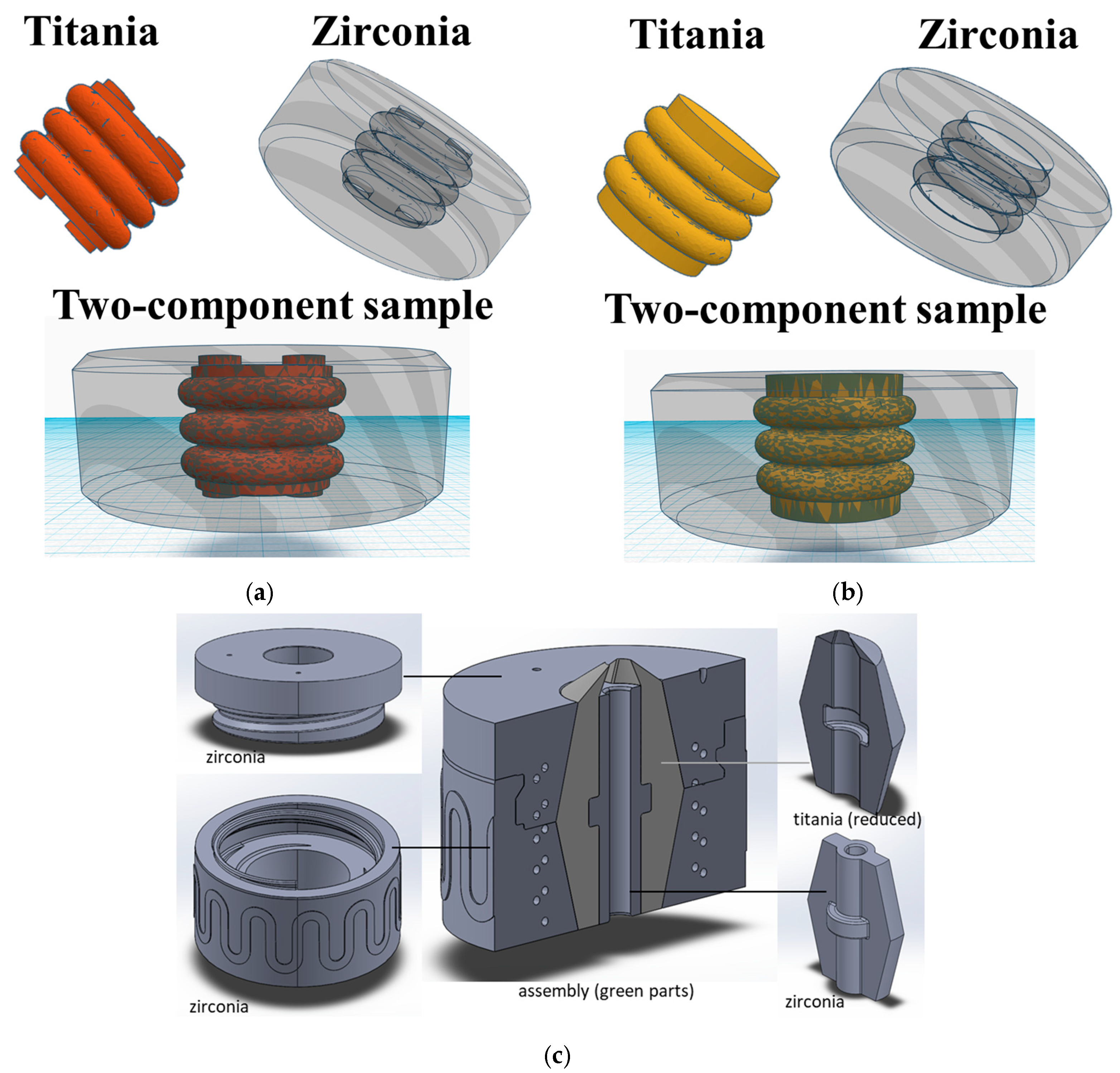
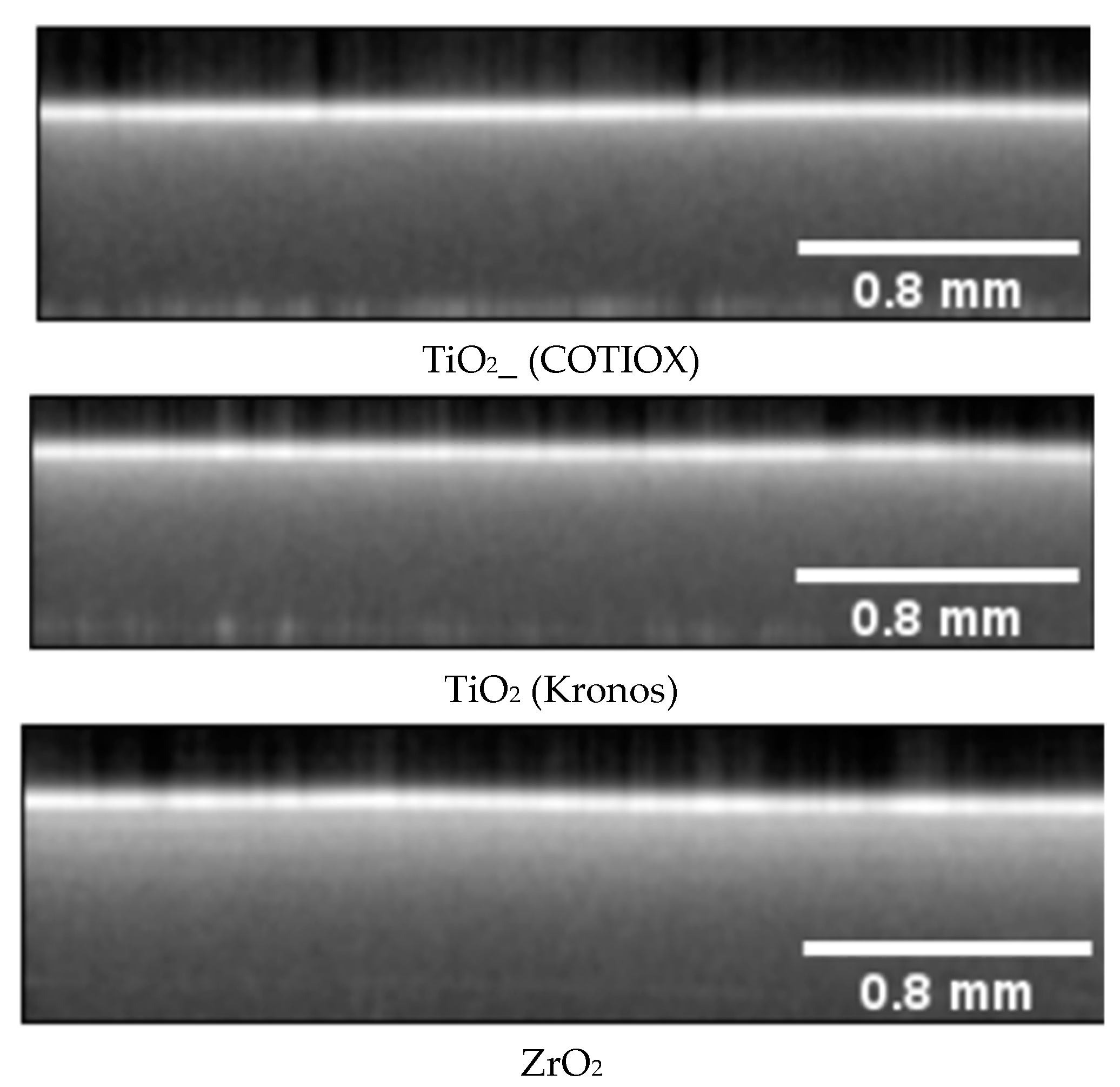
| Single-component samples | TiO2 (Kronos), Lithoz printer [14] TiO2 (COTIOX), Lithoz printer ZrO2, Lithoz printer [14] | - - - |
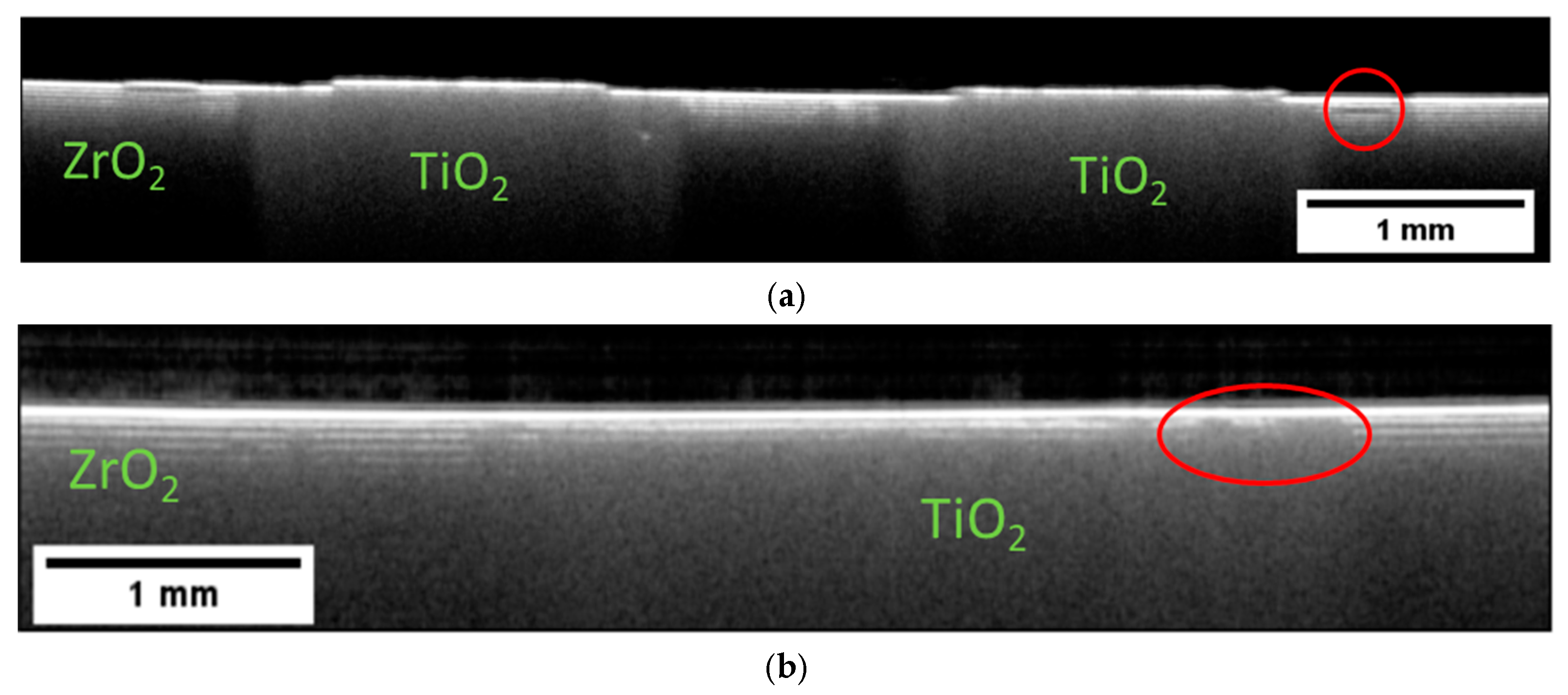
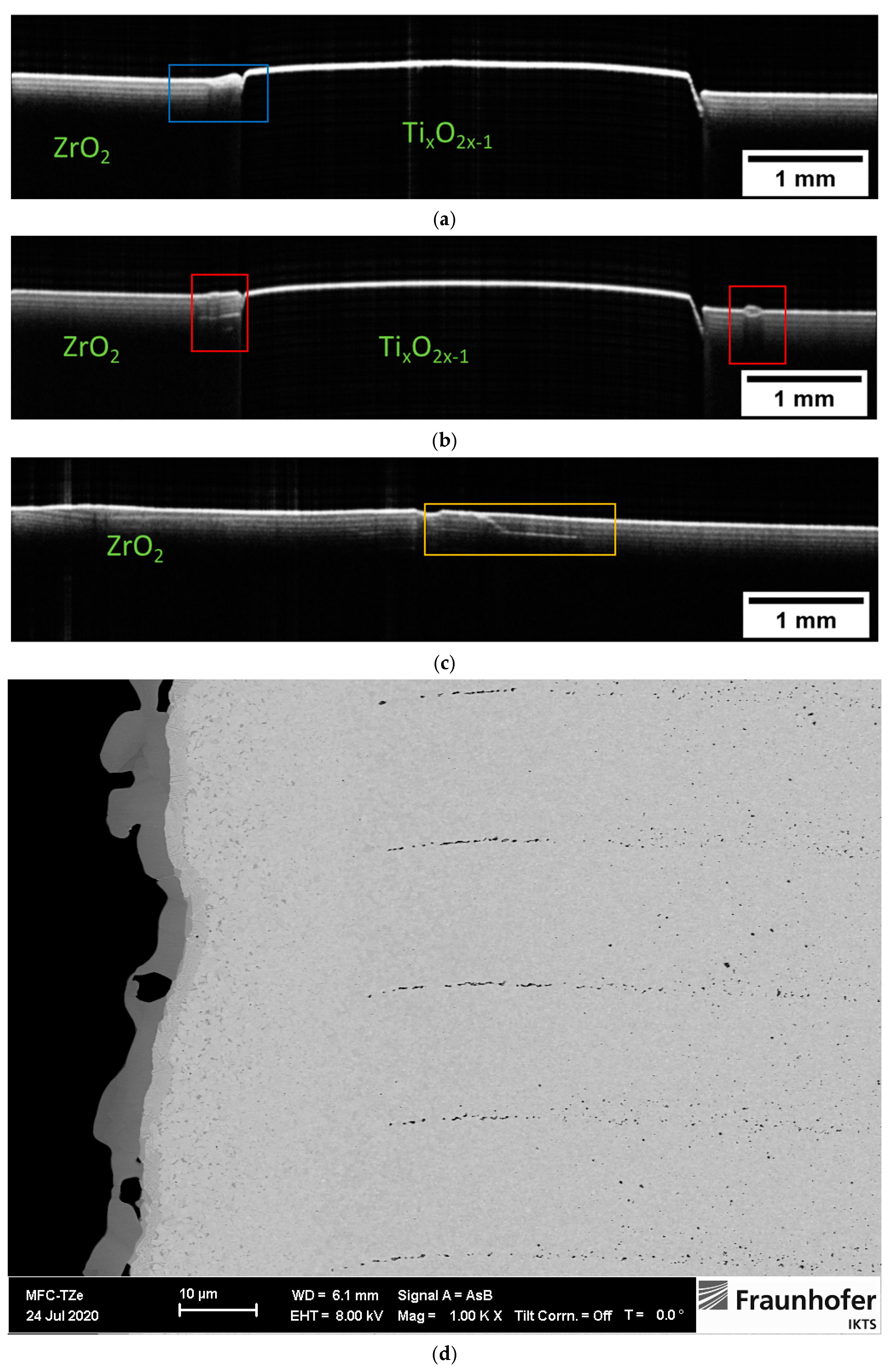
| Two-component samples | TiO2/ZrO2 type 1, Multi-CAMP TiO2/ZrO2 type 2, Multi-CAMP | TiO2/ZrO2 type 1, Multi-CAMP TiO2/ZrO2 type 2, Multi-CAMP TiO2/ZrO2 sintered after assembling single-component elements, Lithoz printer |
Disclaimer/Publisher’s Note: The statements, opinions and data contained in all publications are solely those of the individual author(s) and contributor(s) and not of MDPI and/or the editor(s). MDPI and/or the editor(s) disclaim responsibility for any injury to people or property resulting from any ideas, methods, instructions or products referred to in the content. |
© 2023 by the authors. Licensee MDPI, Basel, Switzerland. This article is an open access article distributed under the terms and conditions of the Creative Commons Attribution (CC BY) license (https://creativecommons.org/licenses/by/4.0/).
Share and Cite
Kopycinska-Müller, M.; Schreiber, L.; Schwarzer-Fischer, E.; Günther, A.; Phillips, C.; Moritz, T.; Opitz, J.; Choi, Y.-J.; Yun, H.-s. Signal-Decay Based Approach for Visualization of Buried Defects in 3-D Printed Ceramic Components Imaged with Help of Optical Coherence Tomography. Materials 2023, 16, 3607. https://doi.org/10.3390/ma16103607
Kopycinska-Müller M, Schreiber L, Schwarzer-Fischer E, Günther A, Phillips C, Moritz T, Opitz J, Choi Y-J, Yun H-s. Signal-Decay Based Approach for Visualization of Buried Defects in 3-D Printed Ceramic Components Imaged with Help of Optical Coherence Tomography. Materials. 2023; 16(10):3607. https://doi.org/10.3390/ma16103607
Chicago/Turabian StyleKopycinska-Müller, Malgorzata, Luise Schreiber, Eric Schwarzer-Fischer, Anne Günther, Conner Phillips, Tassilo Moritz, Jörg Opitz, Yeong-Jin Choi, and Hui-suk Yun. 2023. "Signal-Decay Based Approach for Visualization of Buried Defects in 3-D Printed Ceramic Components Imaged with Help of Optical Coherence Tomography" Materials 16, no. 10: 3607. https://doi.org/10.3390/ma16103607