
Level-Set Modeling of Grain Growth in 316L Stainless Steel under Different Assumptions Regarding Grain Boundary Properties


Abstract
:1. Introduction
2. The Numerical Formulation
GB Velocity Formulation
3. Parameters Identification
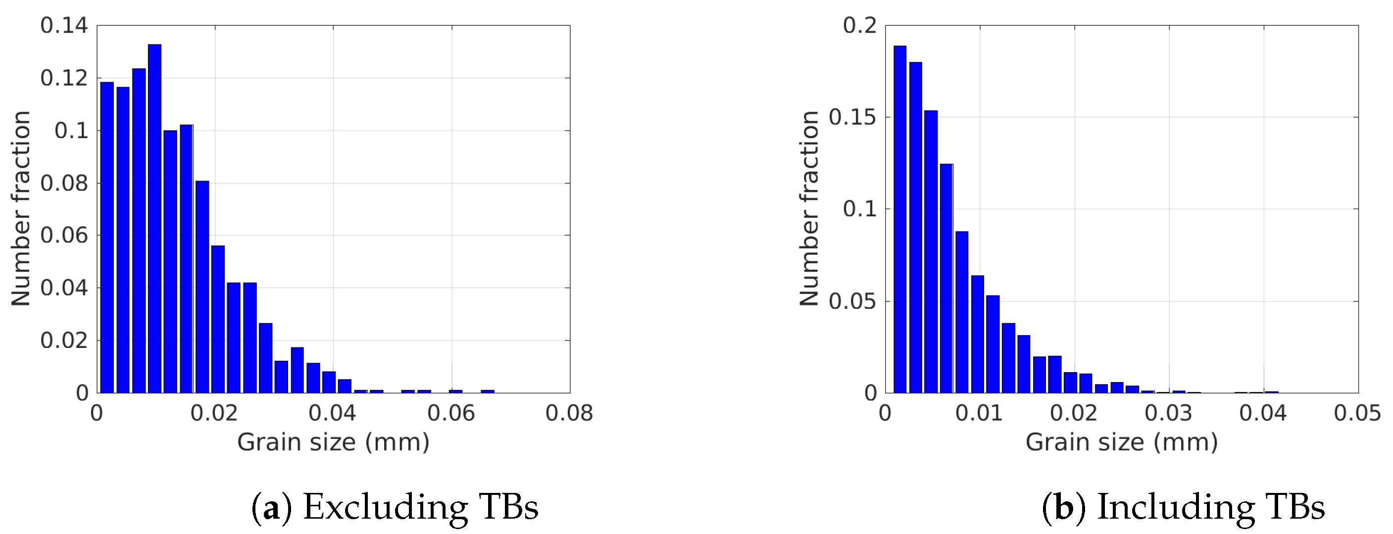
3.1. Material Characterisation
3.2. Estimation of the Average Grain Boundary Mobility Based on the Burke and Turnbull GG Method
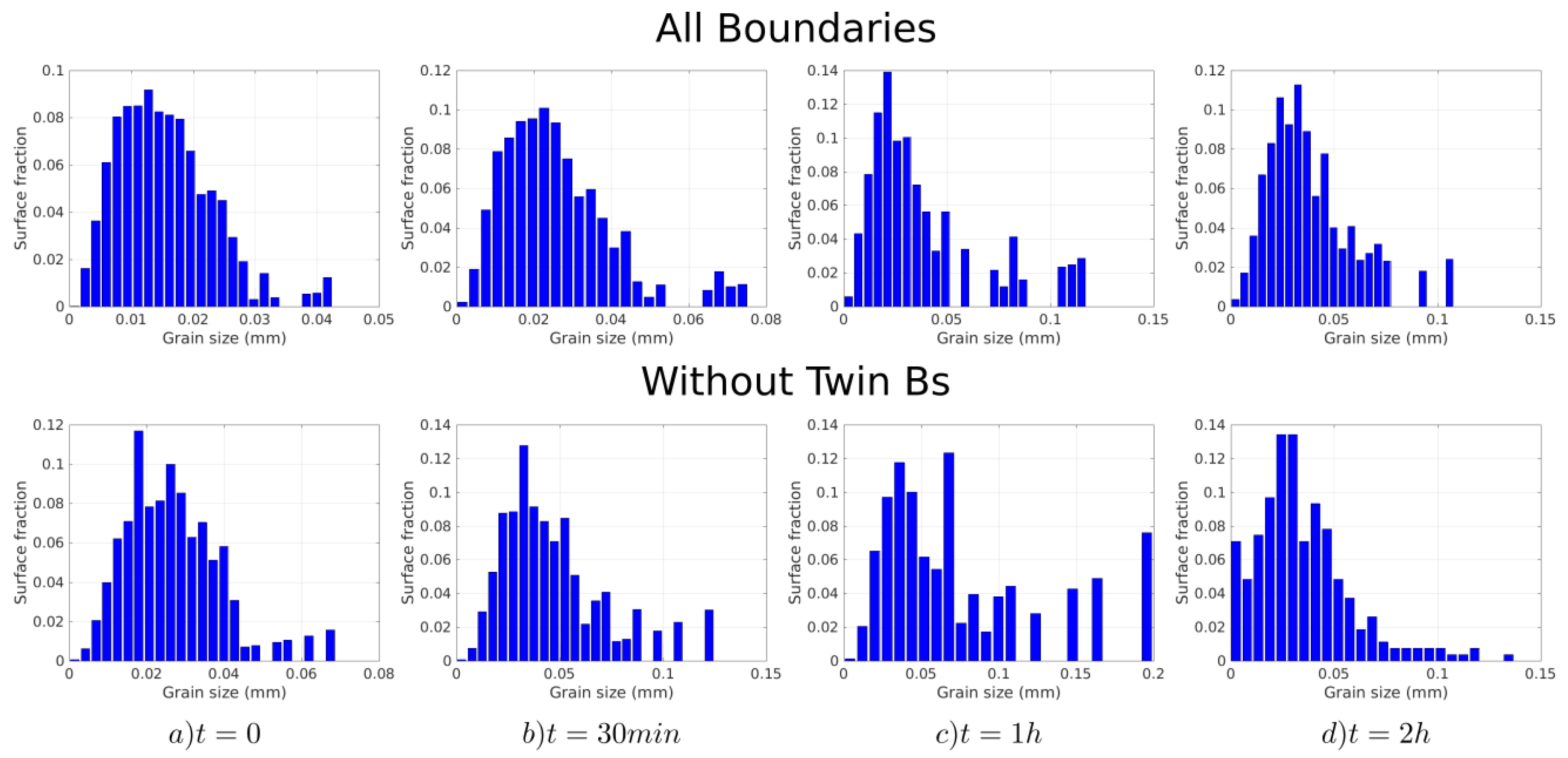
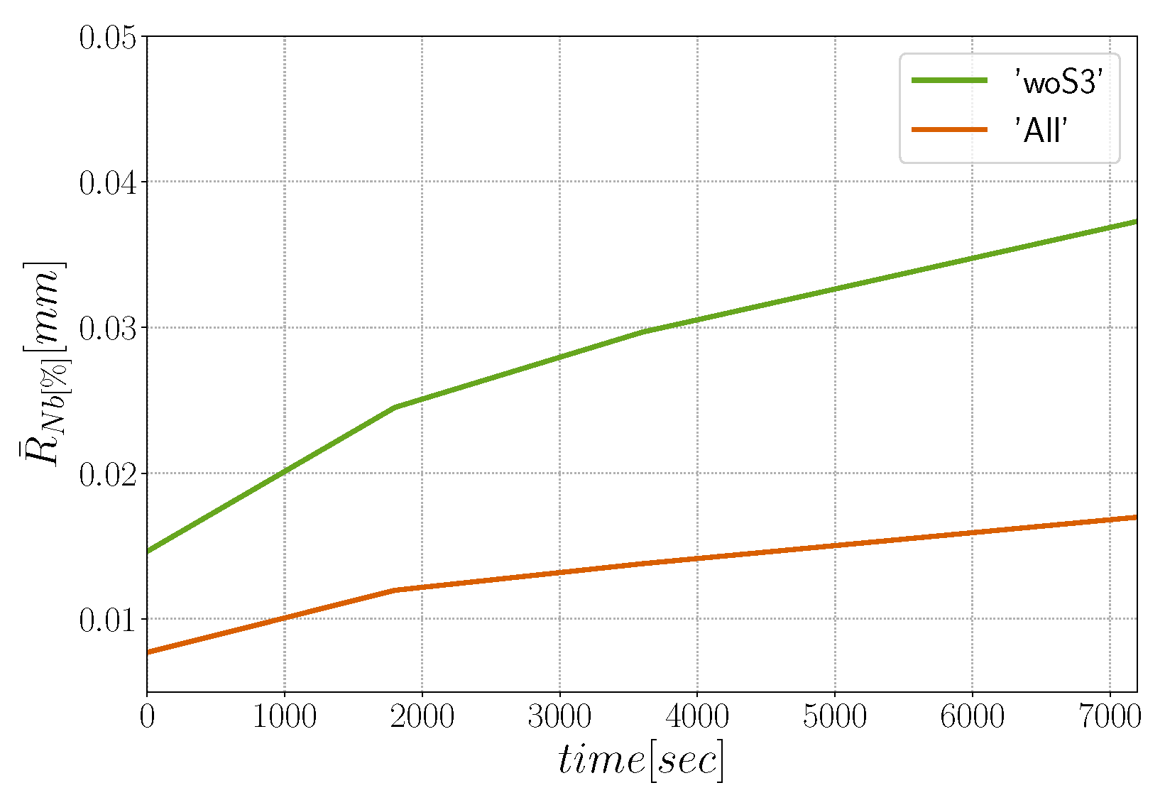
4. Statistical Cases
4.1. Statistical Case with General Boundaries
4.2. Statistical Case with an Improved Description of the and Fields
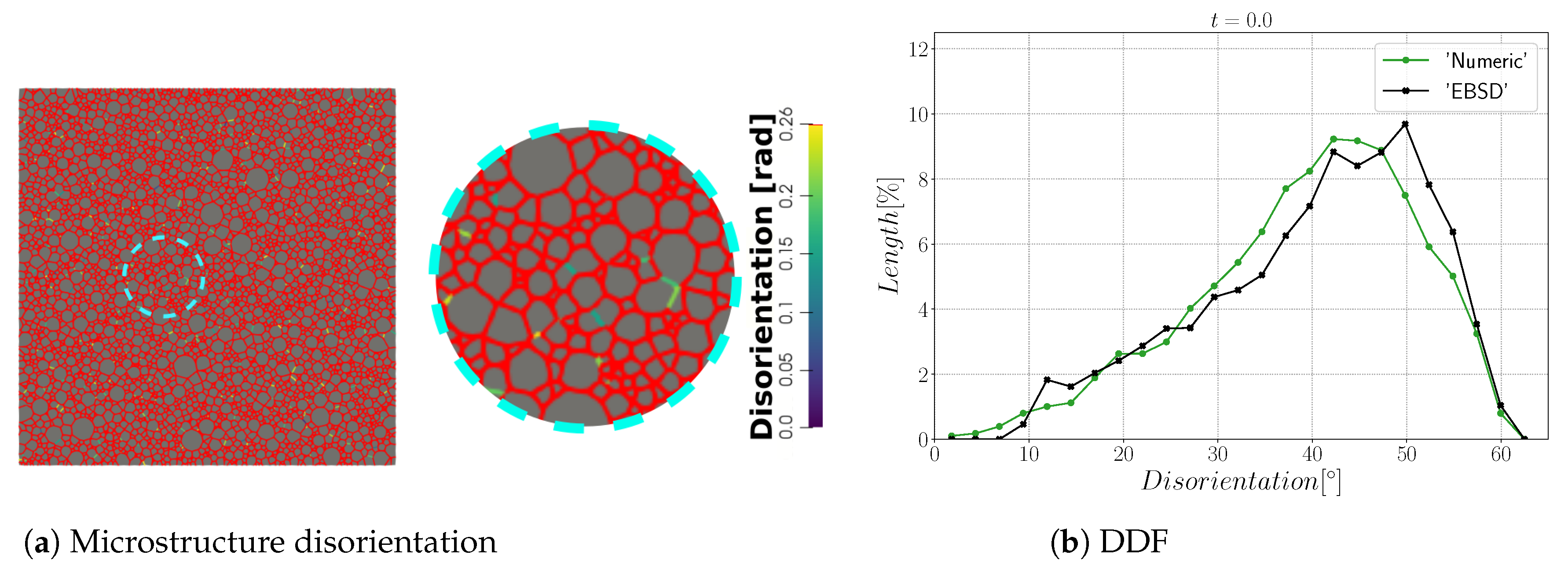
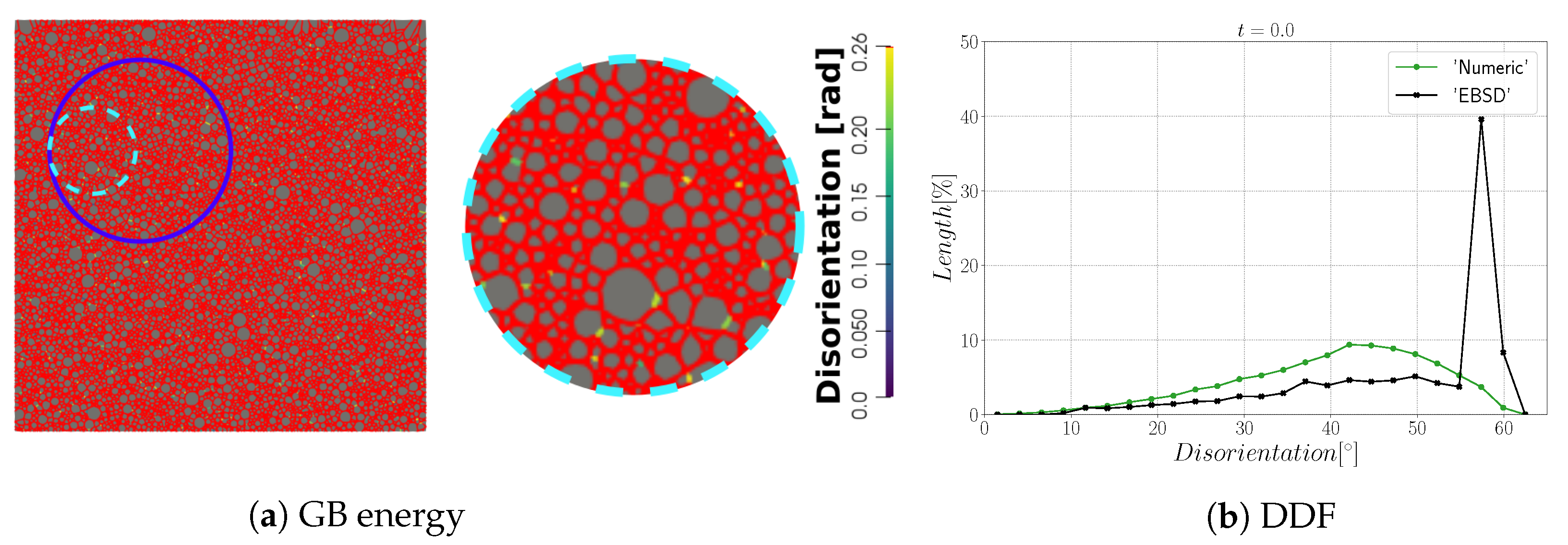
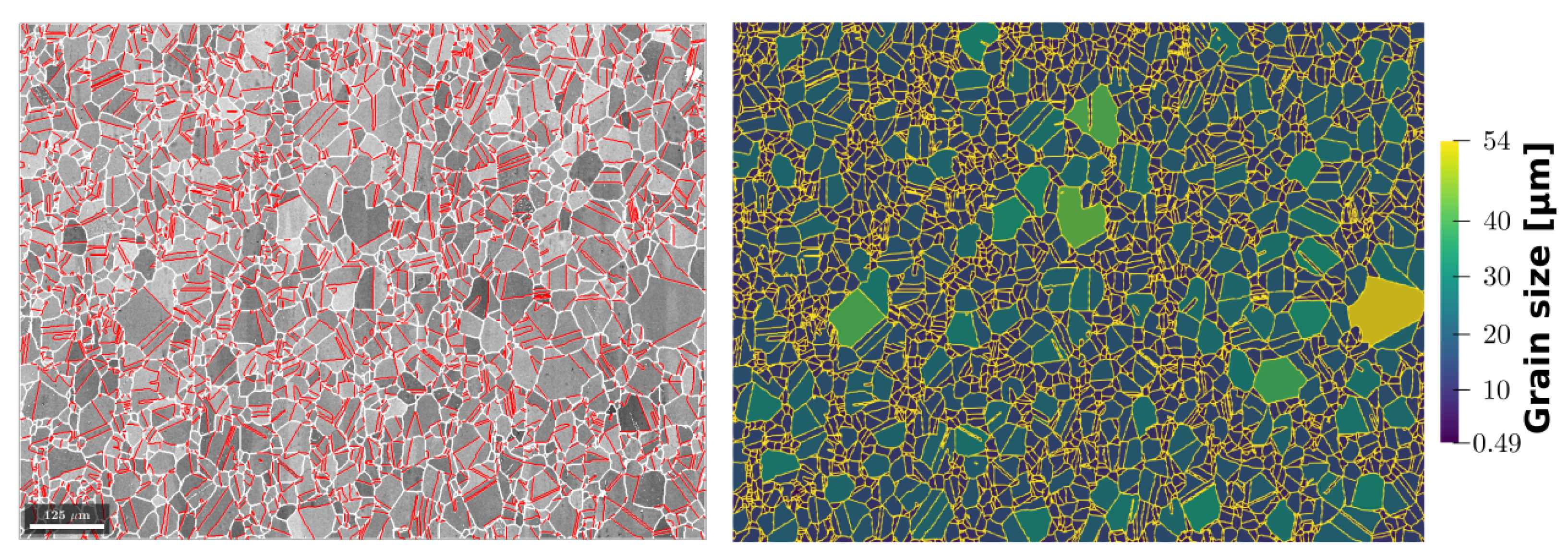
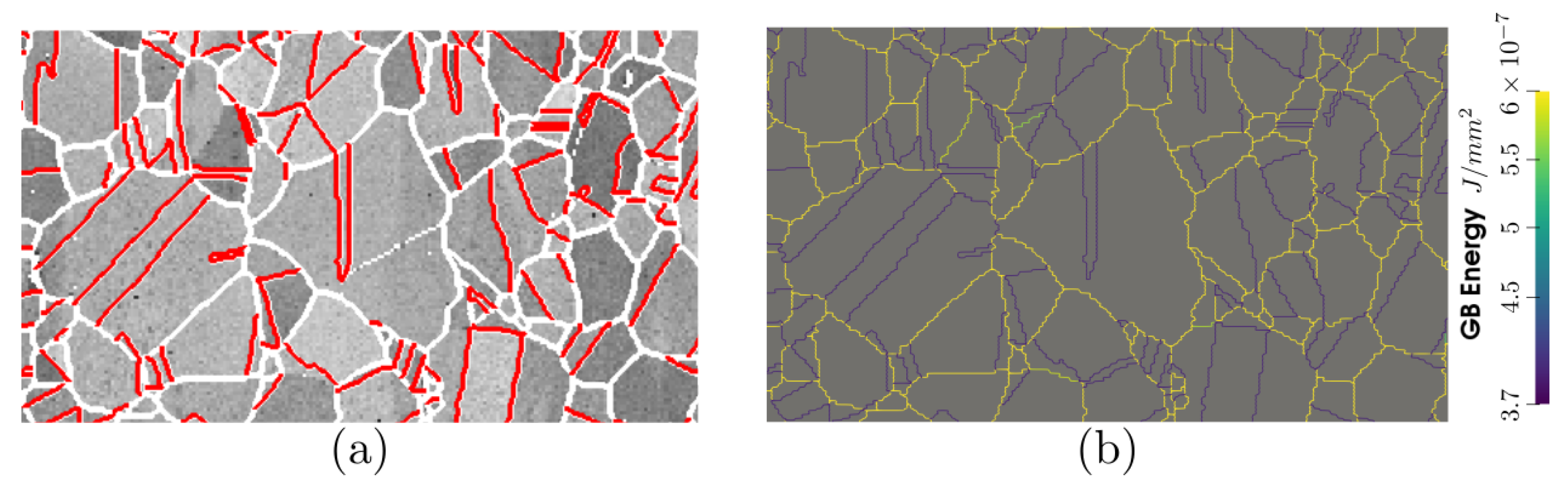
5. Immersion of EBSD Data
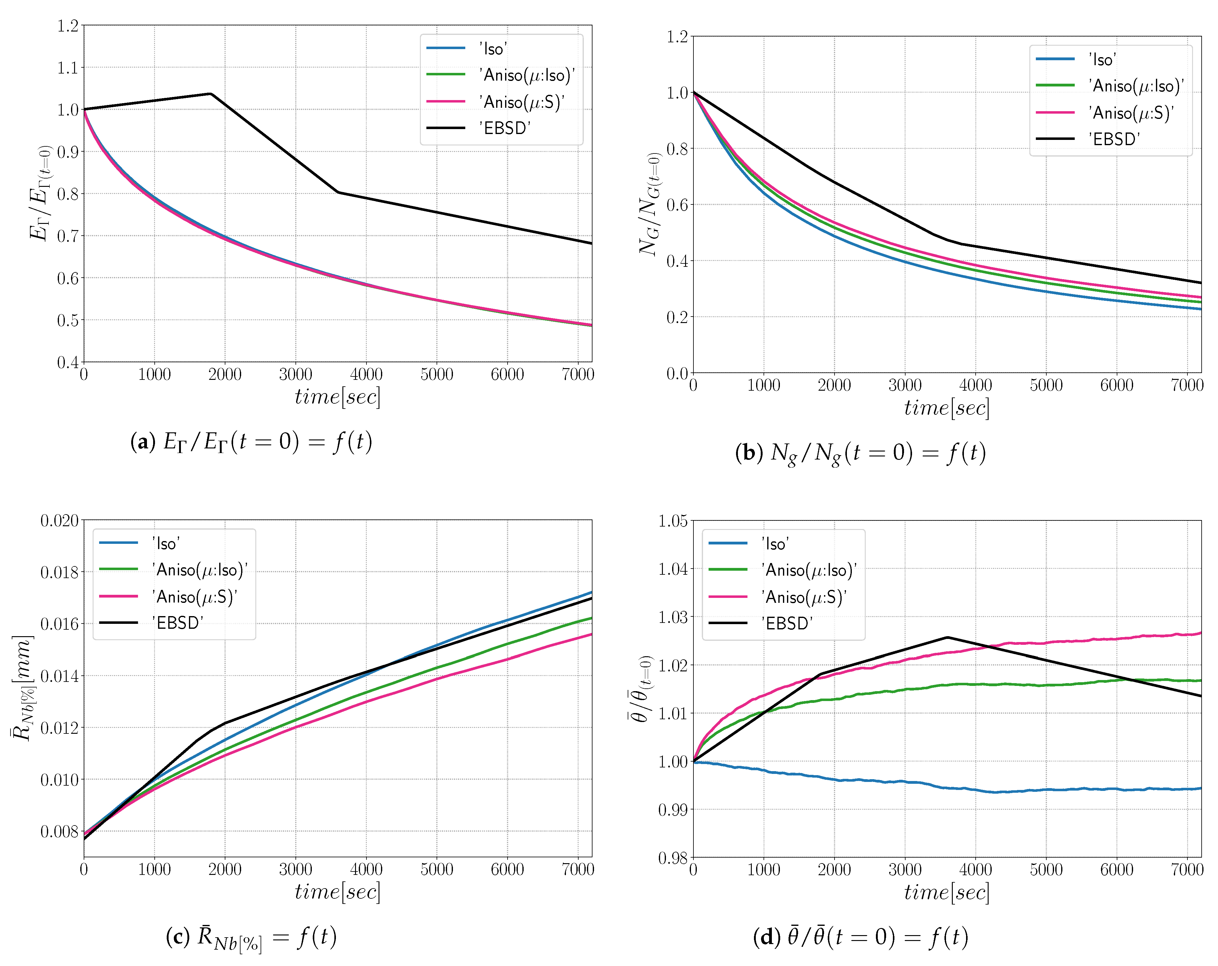
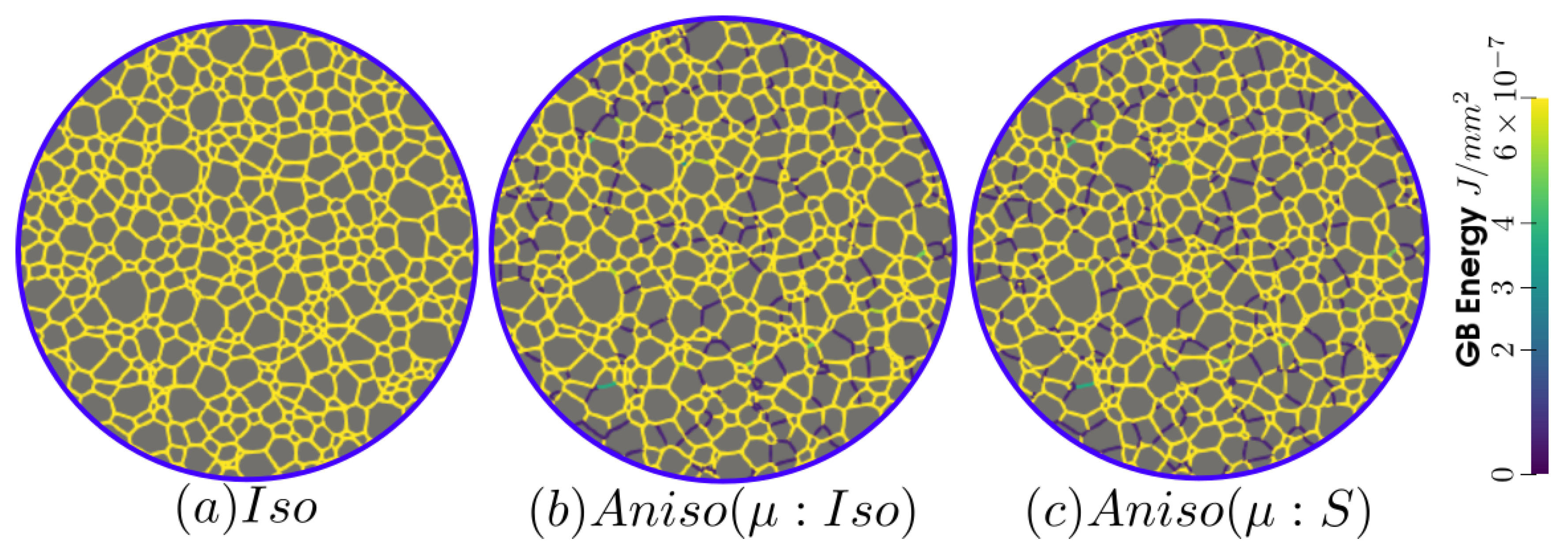
6. Using Anisotropic GB Energy and Heterogeneous GB Mobility
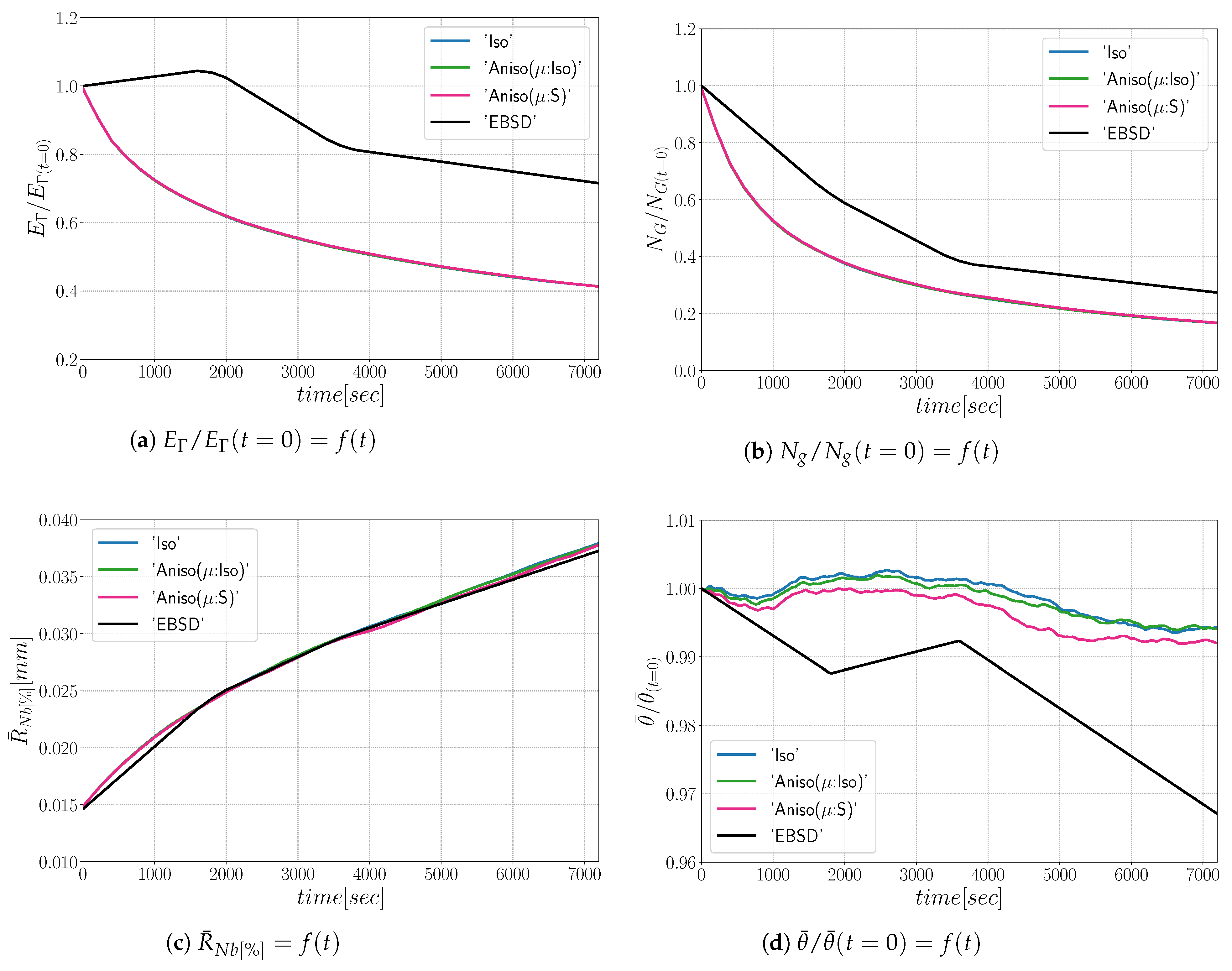
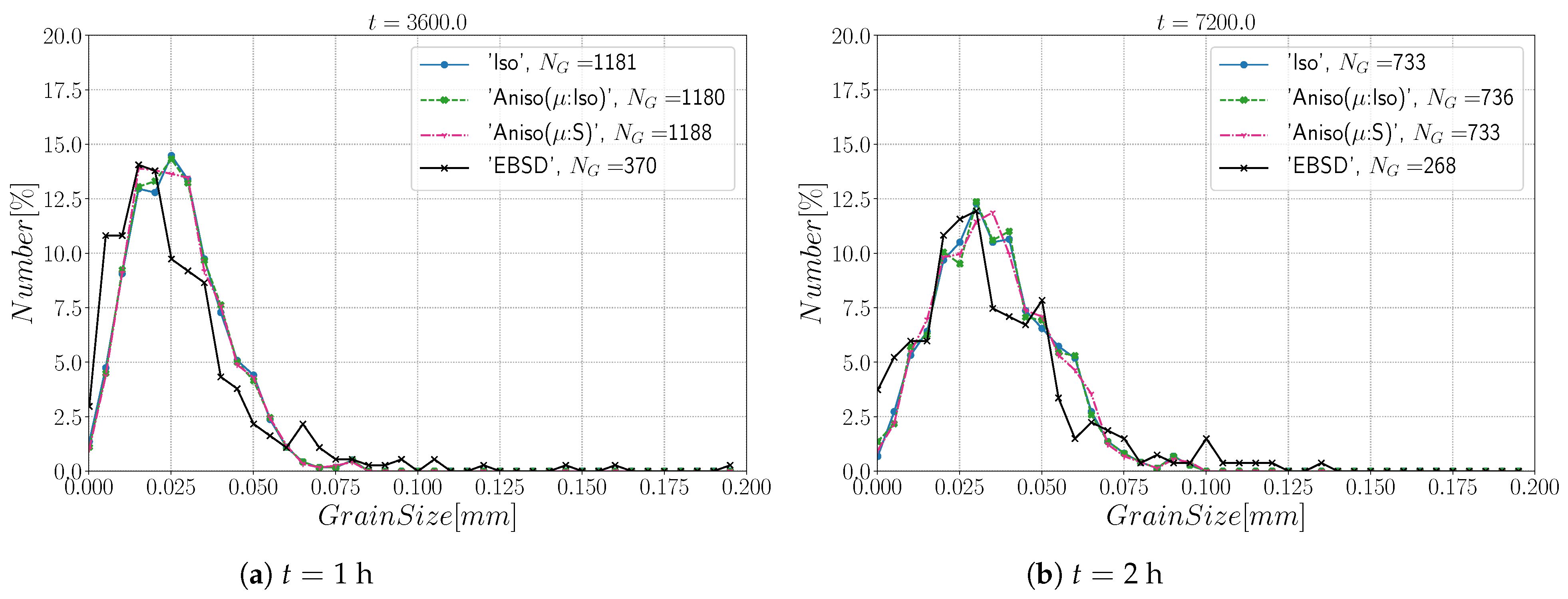
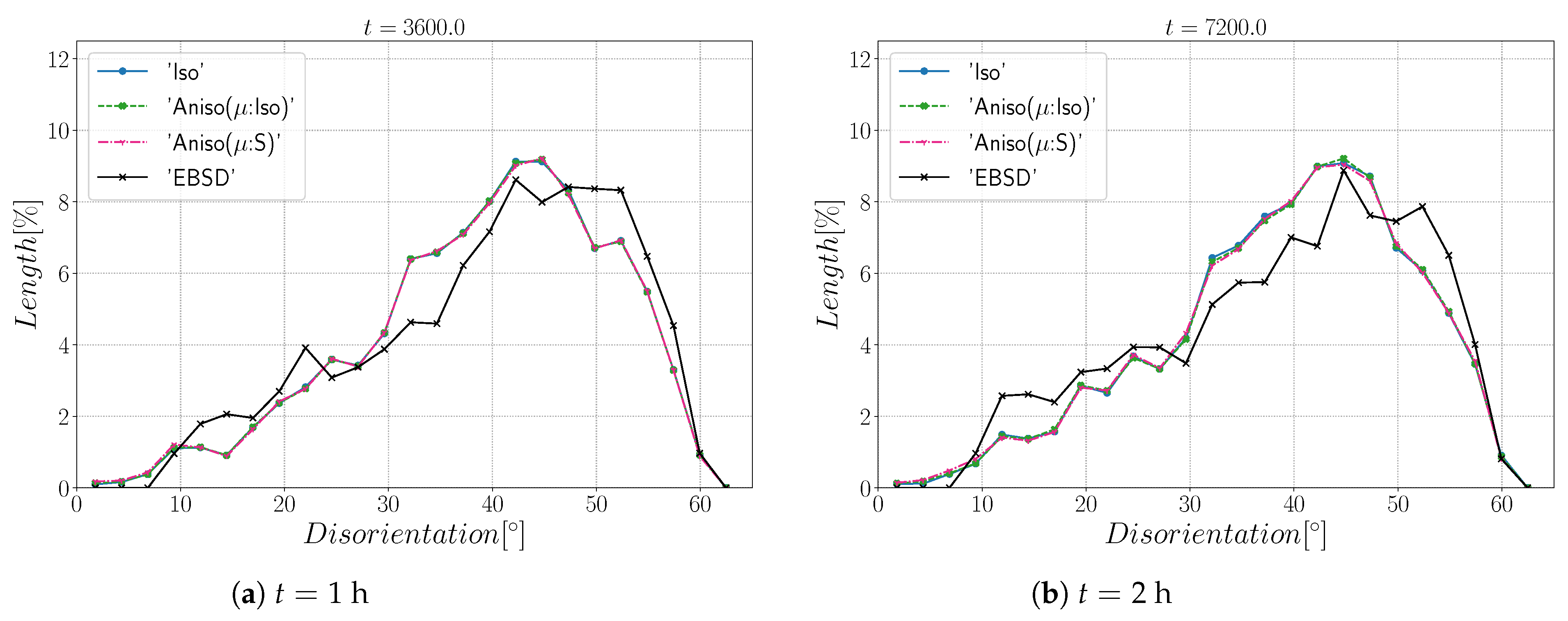
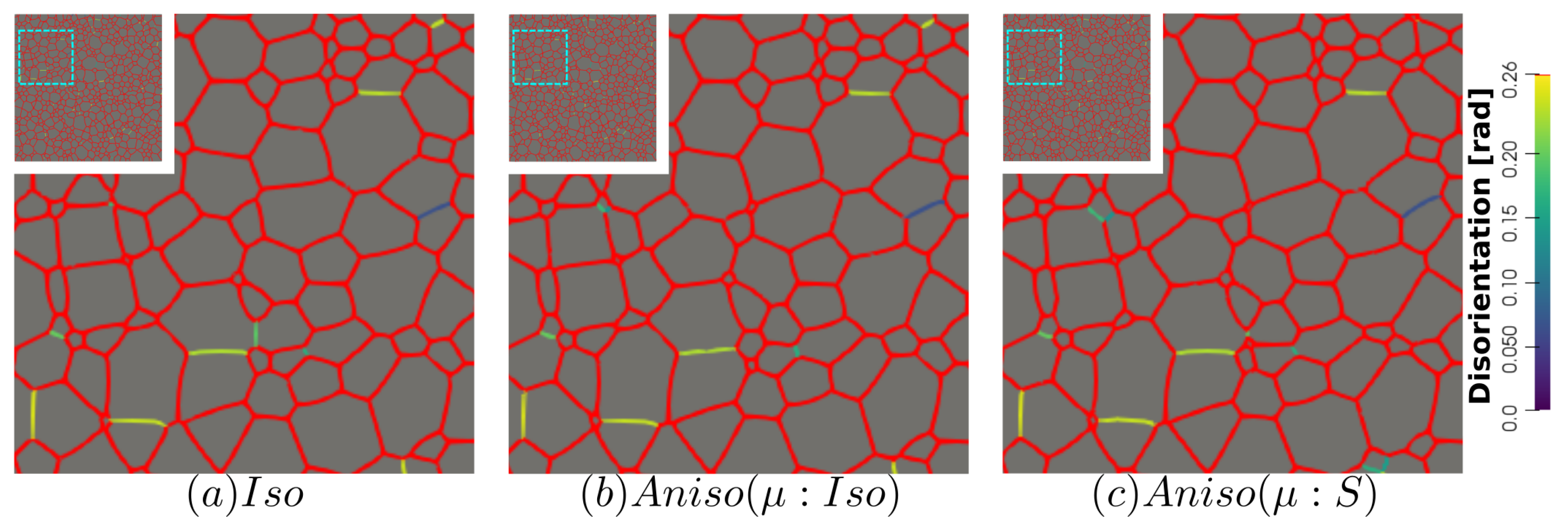
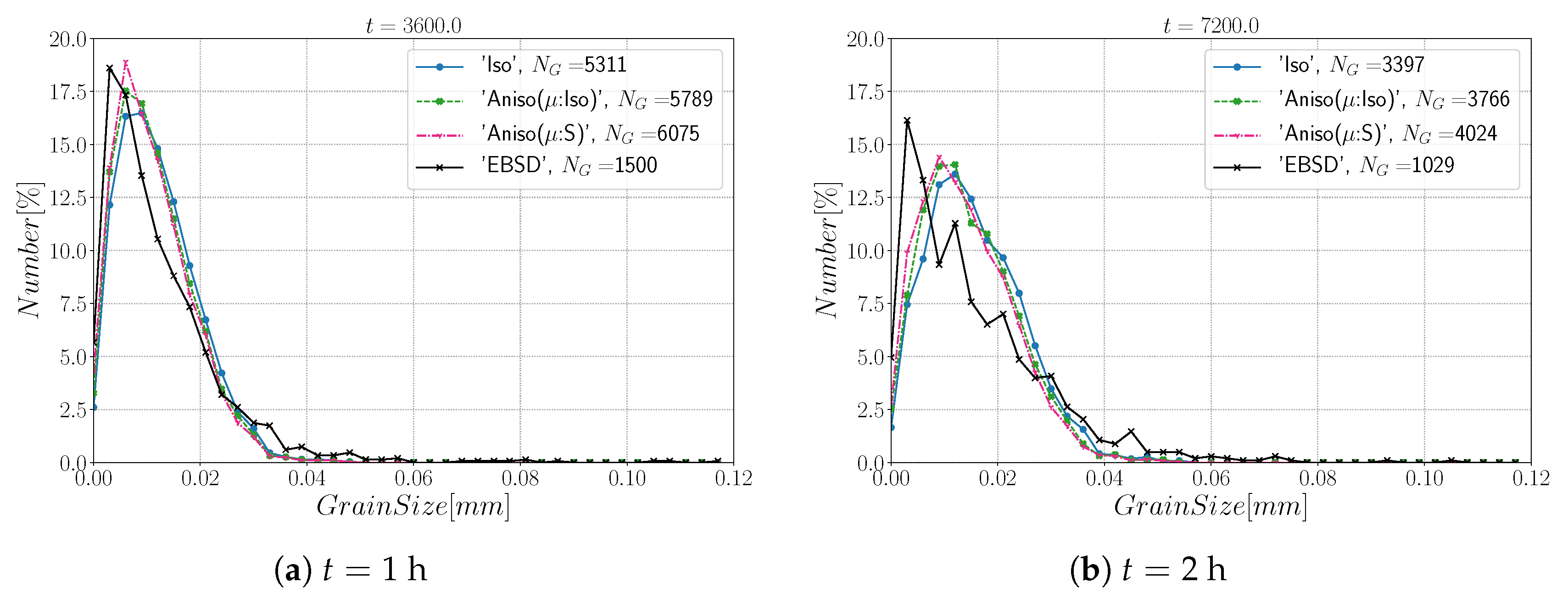
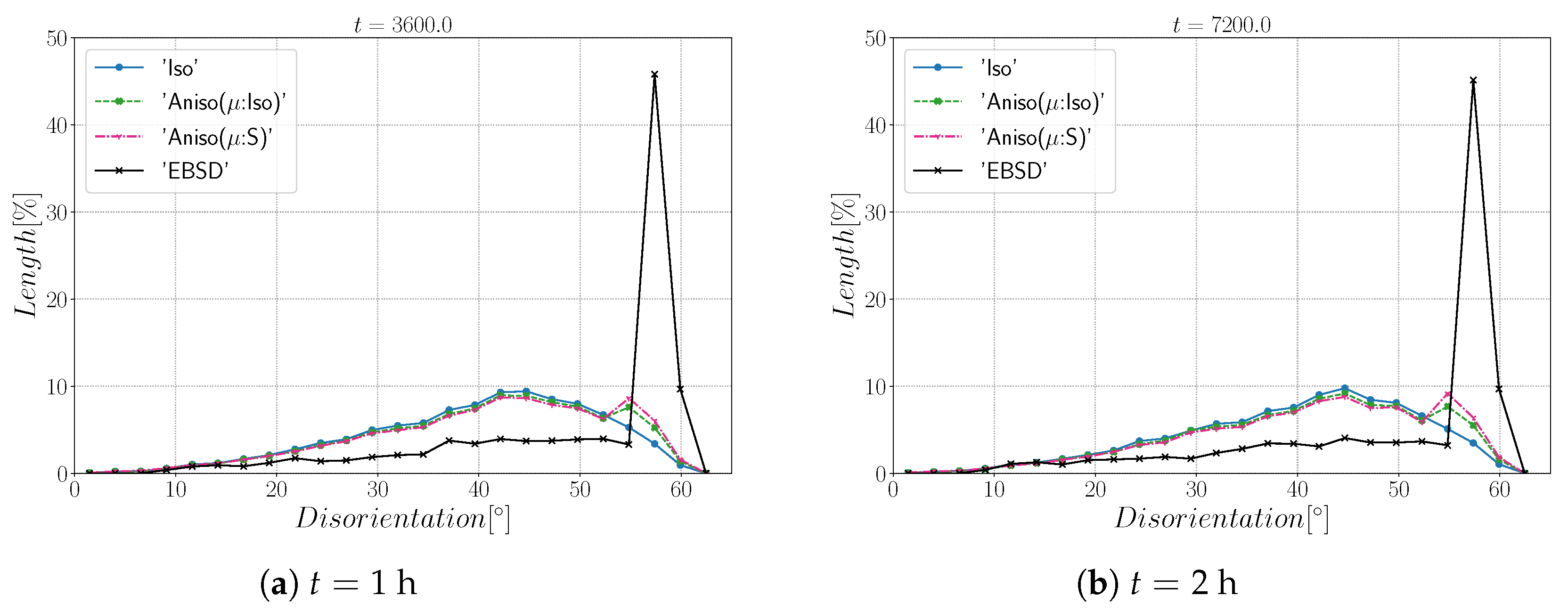
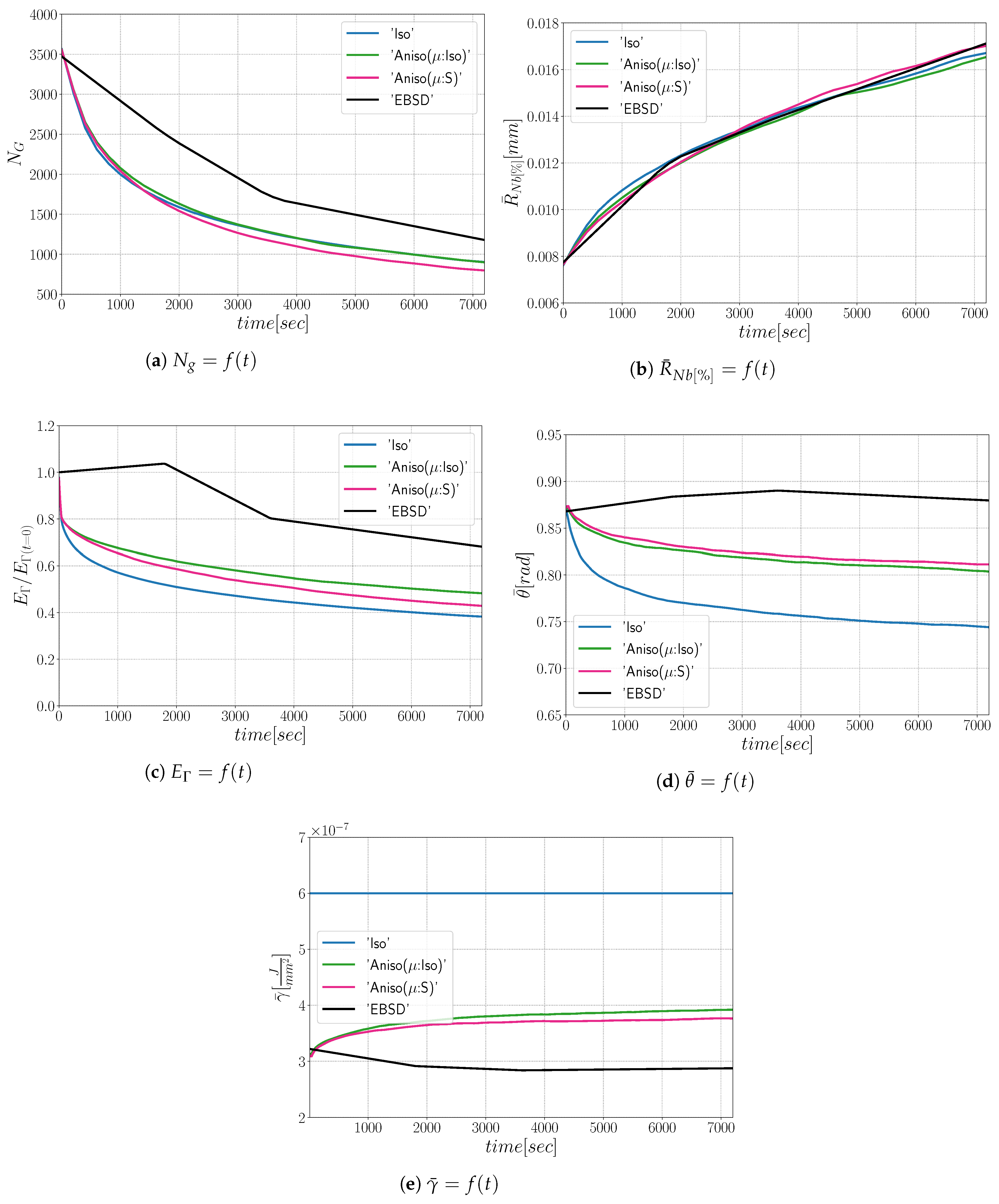
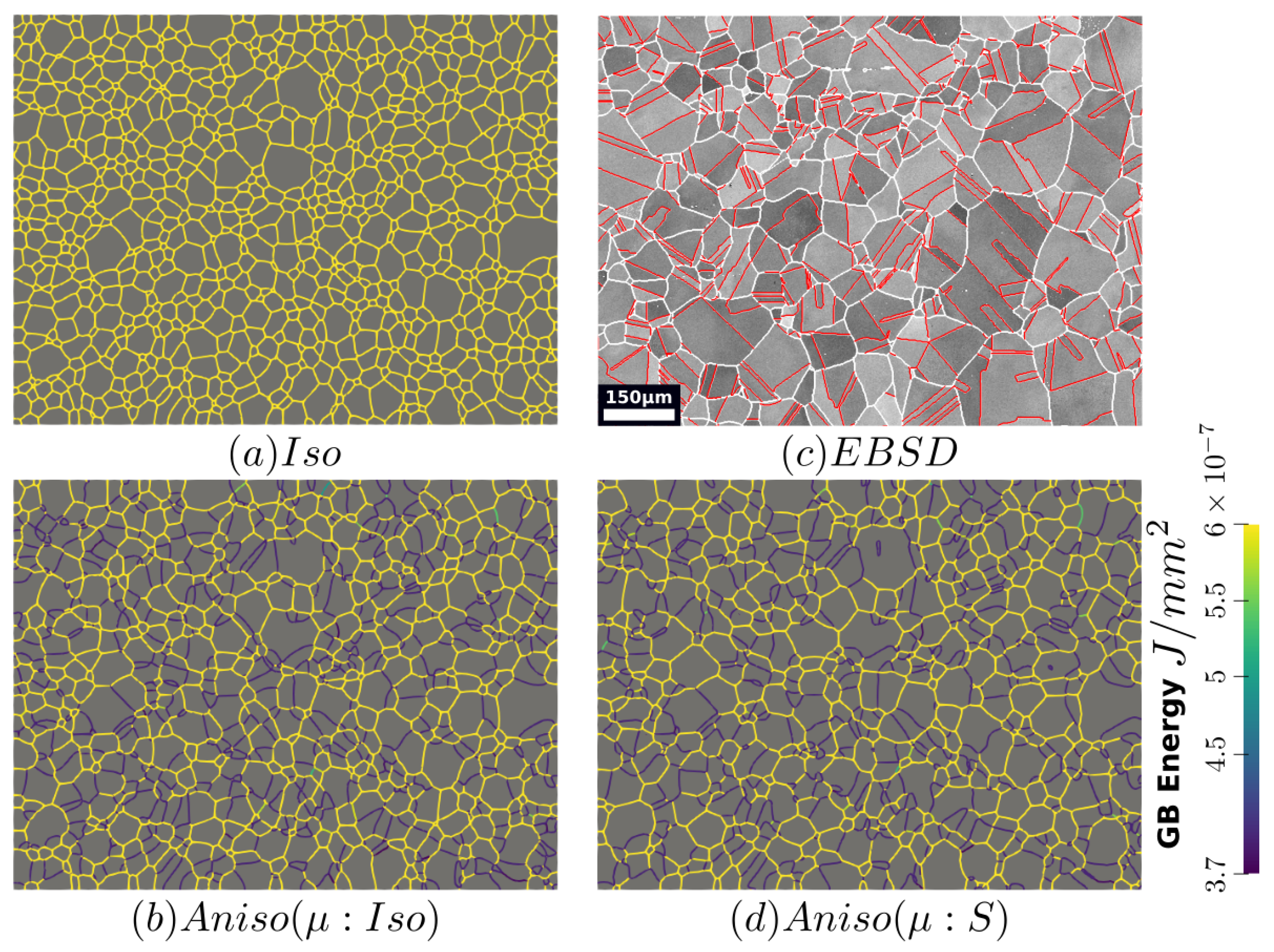
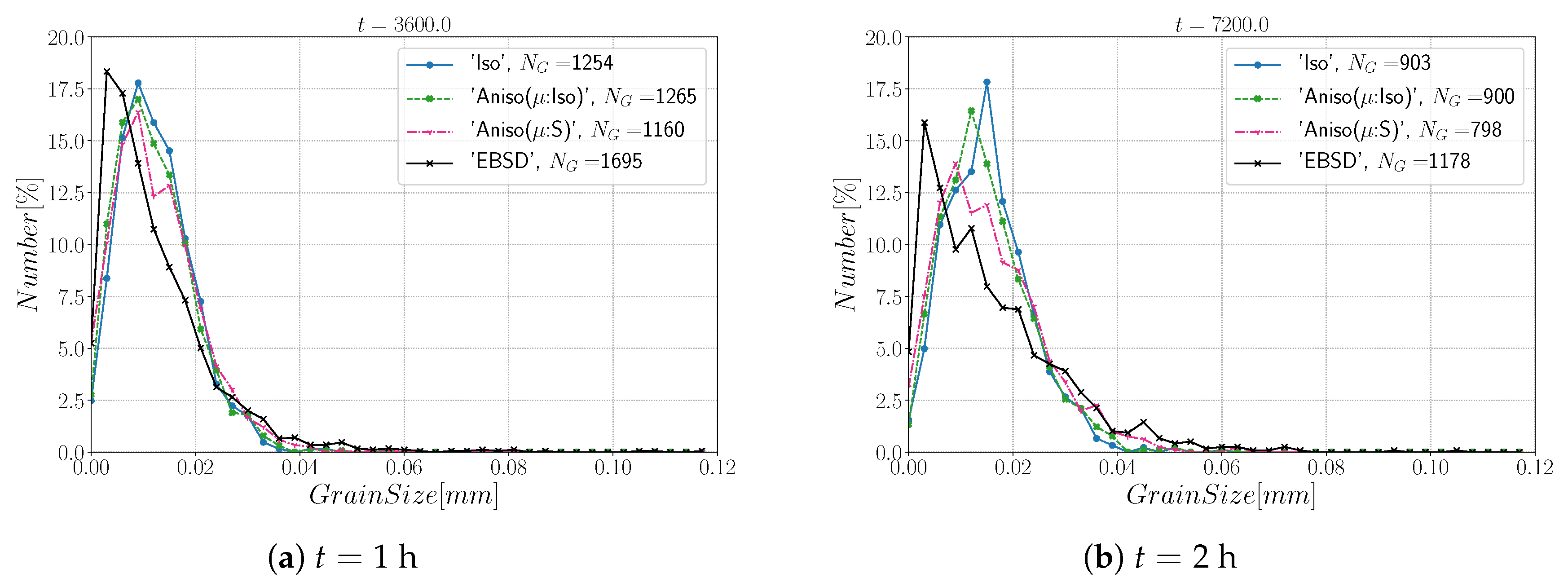
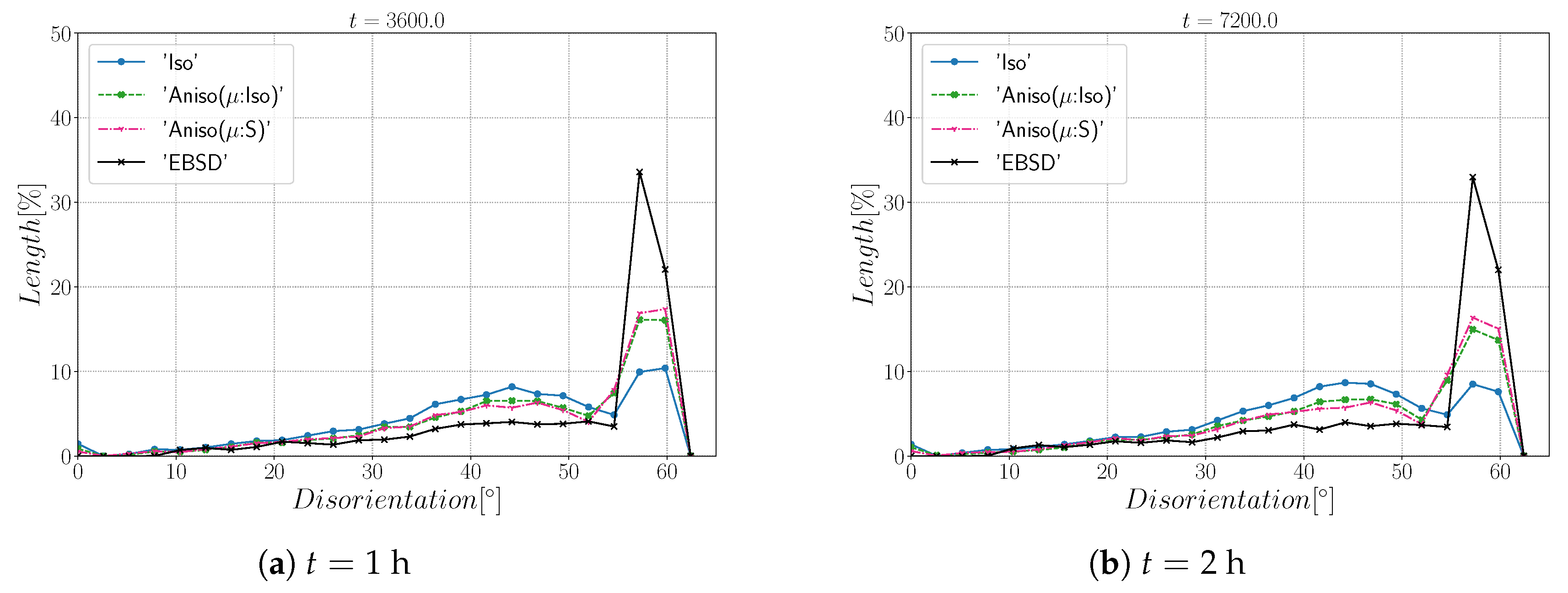
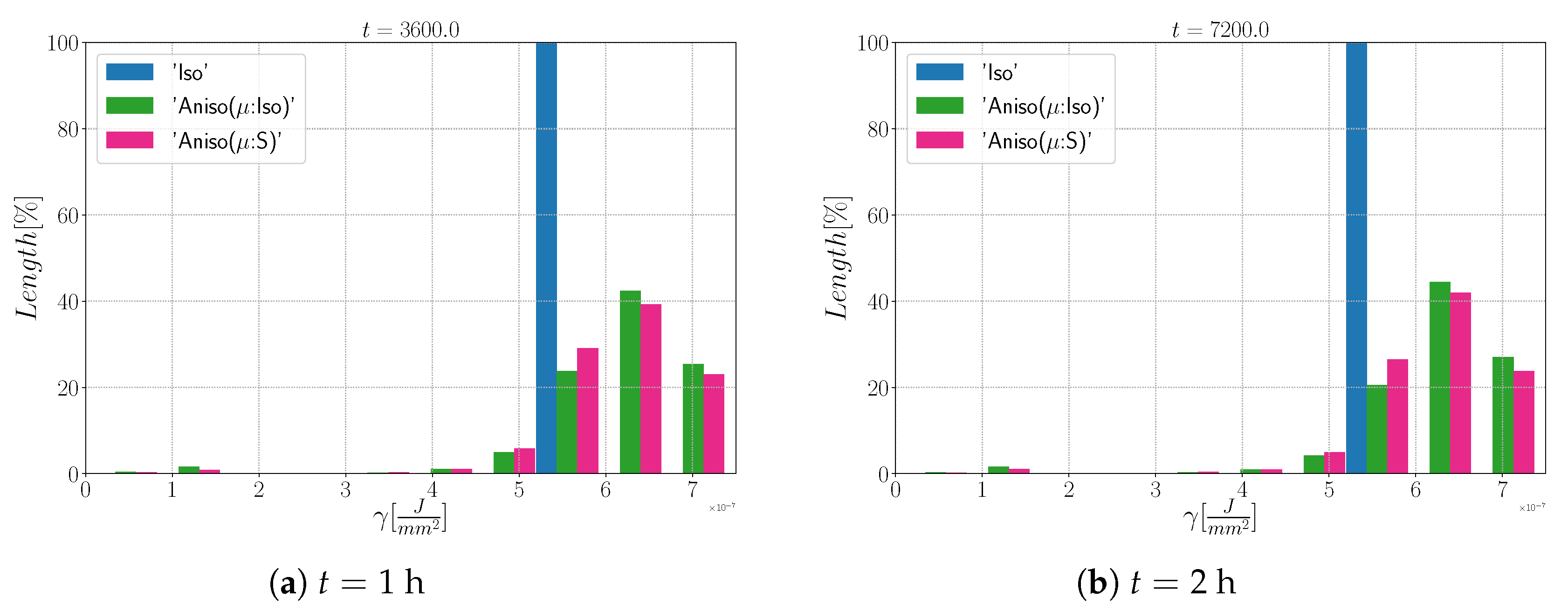
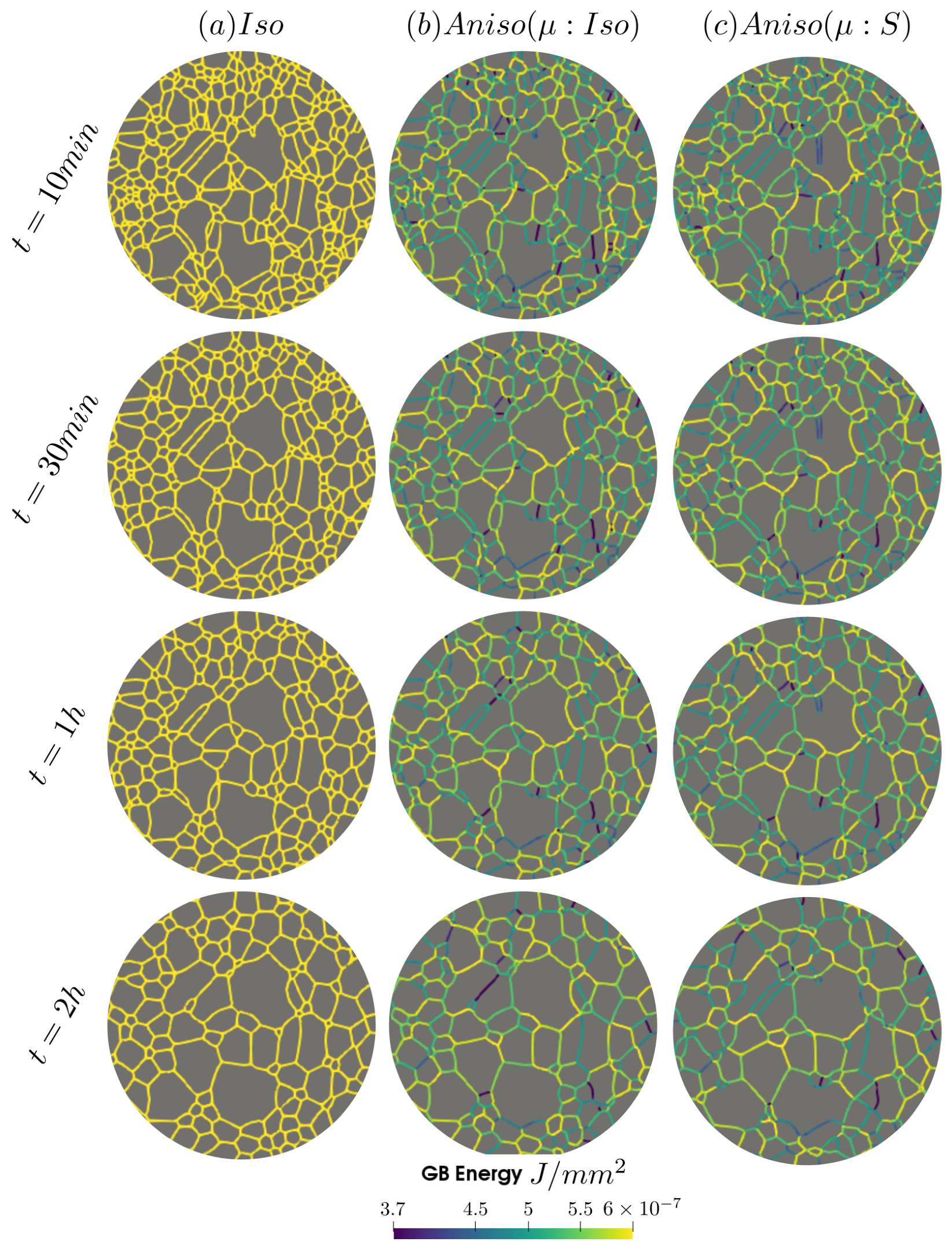
6.1. Simulation Results
6.2. Current State of the Modeling of 3D Anisotropic Grain Growth
- The individual effect of GB energy and mobility is small on the GG [52].
7. Summary and Conclusions
Author Contributions
Funding
Institutional Review Board Statement
Informed Consent Statement
Data Availability Statement
Acknowledgments
Conflicts of Interest
Abbreviations
| Aniso | Anisotropic formulation |
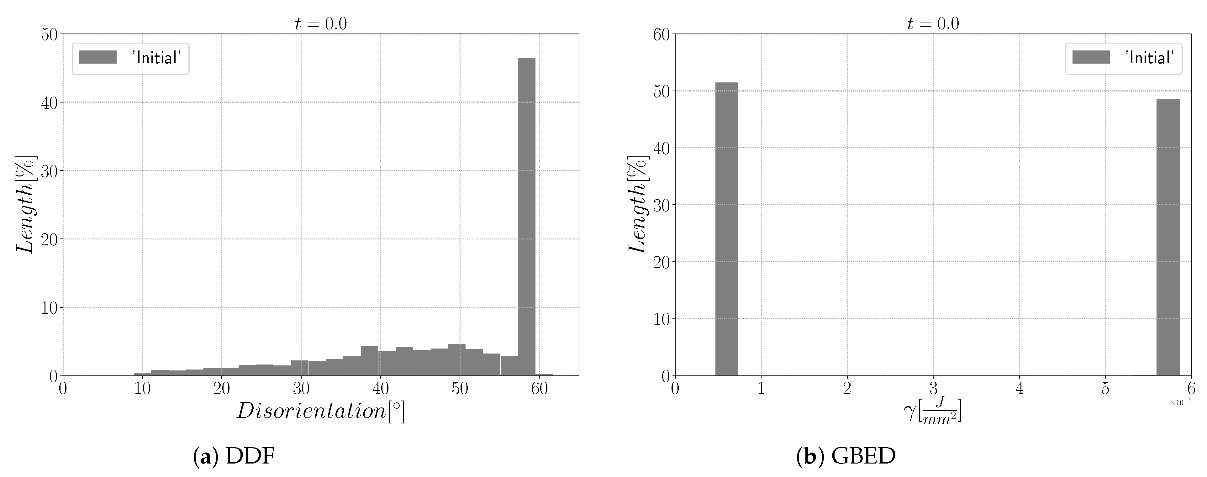
| DDF | Disorientation Distribution Function |
| EBSD | Electron Backscatter Diffraction |
| FE | Finite Element |
| FEGSEM | Field Emission Gun Scanning Electron Microscope |
| FE-LS | Finite Element–Level-Set |
| GB | Grain Boundary |
| GB5DOF | Code to compute the GB energy as a function of the misorientation and normal [6] |
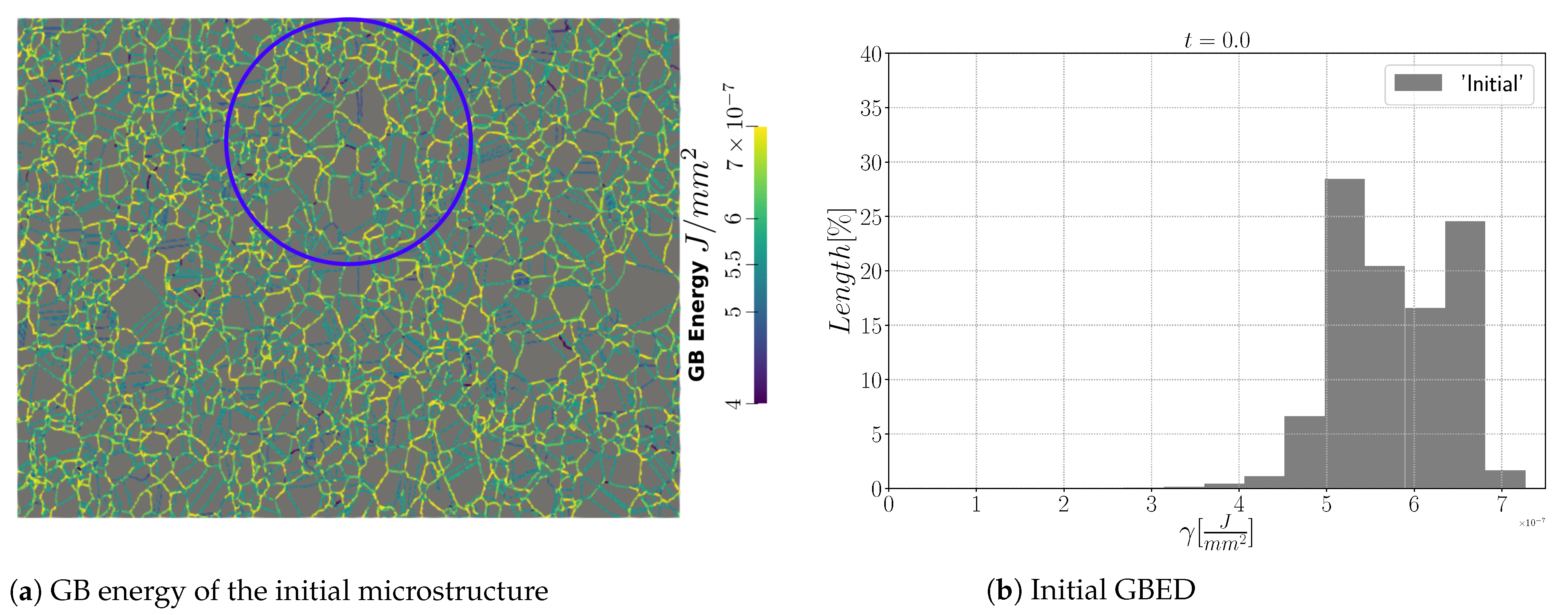
| GBED | Grain Boundary Energy distribution |
| GG | Grain Growth |
| GSD | Grain Size Distribution |
| HAGB | High-Angle Grain Boundary |
| IPF | Inverse Pole Figure |
| Iso | Isotropic formulation |
| LAGB | Low-Angle Grain Boundary |
| LS | Level Set |
| NGG | Normal Grain Growth |
| RS | Read–Shockley |
| S | Sigmoidal |
| TB | Twin Boundary |
References
- Rollett, A.; Rohrer, G.S.; Humphreys, J. Recrystallization and Related Annealing Phenomena; Elsevier: Amsterdam, The Netherlands, 2017. [Google Scholar]
- Bhattacharya, A.; Shen, Y.F.; Hefferan, C.M.; Li, S.F.; Lind, J.; Suter, R.M.; Krill, C.E.; Rohrer, G.S. Grain boundary velocity and curvature are not correlated in Ni polycrystals. Science 2021, 374, 189–193. [Google Scholar] [CrossRef] [PubMed]
- Florez, S.; Alvarado, K.; Murgas, B.; Bozzolo, N.; Chatain, D.; Krill, C.E.; Wang, M.; Rohrer, G.S.; Bernacki, M. Statistical behaviour of interfaces subjected to curvature flow and torque effects applied to microstructural evolutions. Acta Mater. 2022, 222, 117459. [Google Scholar] [CrossRef]
- Olmsted, D.L.; Foiles, S.M.; Holm, E.A. Survey of computed grain boundary properties in face-centered cubic metals: I. Grain boundary energy. Acta Mater. 2009, 57, 3694–3703. [Google Scholar] [CrossRef]
- Olmsted, D.L.; Foiles, S.M.; Holm, E.A. Survey of computed grain boundary properties in face-centered cubic metals: II. Grain boundary mobility. Acta Mater. 2009, 57, 3704–3713. [Google Scholar] [CrossRef]
- Bulatov, V.V.; Reed, B.W.; Kumar, M. Grain boundary energy function for fcc metals. Acta Mater. 2014, 65, 161–175. [Google Scholar] [CrossRef]
- Runnels, B.; Beyerlein, I.J.; Conti, S.; Ortiz, M. An analytical model of interfacial energy based on a lattice-matching interatomic energy. J. Mech. Phys. Solids 2016, 89, 174–193. [Google Scholar] [CrossRef] [Green Version]
- Garcke, H.; Nestler, B.; Stoth, B. A multiphase field concept: Numerical simulations of moving phase boundaries and multiple junctions. SIAM J. Appl. Math. 1999, 60, 295–315. [Google Scholar] [CrossRef] [Green Version]
- Miyoshi, E.; Takaki, T. Multi-phase-field study of the effects of anisotropic grain-boundary properties on polycrystalline grain growth. J. Cryst. Growth 2017, 474, 160–165. [Google Scholar] [CrossRef]
- Moelans, N.; Wendler, F.; Nestler, B. Comparative study of two phase-field models for grain growth. Comput. Mater. Sci. 2009, 46, 479–490. [Google Scholar] [CrossRef]
- Gao, J.; Thompson, R. Real time-temperature models for Monte Carlo simulations of normal grain growth. Acta Mater. 1996, 44, 4565–4570. [Google Scholar] [CrossRef]
- Upmanyu, M.; Hassold, G.N.; Kazaryan, A.; Holm, E.A.; Wang, Y.; Patton, B.; Srolovitz, D.J. Boundary mobility and energy anisotropy effects on microstructural evolution during grain growth. Interface Sci. 2002, 10, 201–216. [Google Scholar] [CrossRef]
- Hoffrogge, P.W.; Barrales-Mora, L.A. Grain-resolved kinetics and rotation during grain growth of nanocrystalline aluminium by molecular dynamics. Comput. Mater. Sci. 2017, 128, 207–222. [Google Scholar] [CrossRef] [Green Version]
- Sakout, S.; Weisz-Patrault, D.; Ehrlacher, A. Energetic upscaling strategy for grain growth. i: Fast mesoscopic model based on dissipation. Acta Mater. 2020, 196, 261–279. [Google Scholar] [CrossRef]
- Barrales Mora, L.A. 2D vertex modeling for the simulation of grain growth and related phenomena. Math. Comput. Simul. 2010, 80, 1411–1427. [Google Scholar] [CrossRef]
- Wakai, F.; Enomoto, N.; Ogawa, H. Three-dimensional microstructural evolution in ideal grain growth—General statistics. Acta Mater. 2000, 48, 1297–1311. [Google Scholar] [CrossRef]
- Florez, S.; Shakoor, M.; Toulorge, T.; Bernacki, M. A new finite element strategy to simulate microstructural evolutions. Comput. Mater. Sci. 2020, 172, 109335. [Google Scholar] [CrossRef]
- Florez, S.; Alvarado, K.; Muñoz, D.P.; Bernacki, M. A novel highly efficient Lagrangian model for massively multidomain simulation applied to microstructural evolutions. Comput. Methods Appl. Mech. Eng. 2020, 367, 113107. [Google Scholar] [CrossRef]
- Bernacki, M.; Logé, R.E.; Coupez, T. Level set framework for the finite-element modeling of recrystallization and grain growth in polycrystalline materials. Scr. Mater. 2011, 64, 525–528. [Google Scholar] [CrossRef]
- Mießen, C.; Liesenjohann, M.; Barrales-Mora, L.; Shvindlerman, L.; Gottstein, G. An advanced level set approach to grain growth–Accounting for grain boundary anisotropy and finite triple junction mobility. Acta Mater. 2015, 99, 39–48. [Google Scholar] [CrossRef]
- Fausty, J.; Bozzolo, N.; Bernacki, M. A 2D level set finite element grain coarsening study with heterogeneous grain boundary energies. Appl. Math. Model. 2020, 78, 505–518. [Google Scholar] [CrossRef]
- Murgas, B.; Florez, S.; Bozzolo, N.; Fausty, J.; Bernacki, M. Comparative Study and Limits of Different Level-Set Formulations for the Modeling of Anisotropic Grain Growth. Materials 2021, 14, 3883. [Google Scholar] [CrossRef] [PubMed]
- Kim, J.; Jacobs, M.; Osher, S.; Admal, N.C. A crystal symmetry-invariant Kobayashi–Warren–Carter grain boundary model and its implementation using a thresholding algorithm. arXiv 2021, arXiv:2102.02773. [Google Scholar] [CrossRef]
- Smith, C.S. Introduction to Grains, Phases, and Interfaces—An Interpretation of Microstructure. Trans. Am. Inst. Min. Metall. Eng. 1948, 175, 15–51. [Google Scholar]
- Kohara, S.; Parthasarathi, M.N.; Beck, P.A. Anisotropy of boundary mobility. J. Appl. Phys. 1958, 29, 1125–1126. [Google Scholar] [CrossRef]
- Anderson, M.; Srolovitz, D.; Grest, G.; Sahni, P. Computer simulation of grain growth—I. Kinetics. Acta Metall. 1984, 32, 783–791. [Google Scholar] [CrossRef]
- Lazar, E.A.; Mason, J.K.; MacPherson, R.D.; Srolovitz, D.J. A more accurate three-dimensional grain growth algorithm. Acta Mater. 2011, 59, 6837–6847. [Google Scholar] [CrossRef]
- Rollett, A.; Srolovitz, D.J.; Anderson, M. Simulation and theory of abnormal grain growth—Anisotropic grain boundary energies and mobilities. Acta Metall. 1989, 37, 1227–1240. [Google Scholar] [CrossRef] [Green Version]
- Hwang, N.M. Simulation of the effect of anisotropic grain boundary mobility and energy on abnormal grain growth. J. Mater. Sci. 1998, 33, 5625–5629. [Google Scholar] [CrossRef]
- Fausty, J.; Bozzolo, N.; Pino Muñoz, D.; Bernacki, M. A novel Level-Set Finite Element formulation for grain growth with heterogeneous grain boundary energies. Mater. Des. 2018, 160, 578–590. [Google Scholar] [CrossRef]
- Zöllner, D.; Zlotnikov, I. Texture Controlled Grain Growth in Thin Films Studied by 3D Potts Model. Adv. Theory Simul. 2019, 2, 1900064. [Google Scholar] [CrossRef]
- Miyoshi, E.; Takaki, T. Validation of a novel higher-order multi-phase-field model for grain-growth simulations using anisotropic grain-boundary properties. Comput. Mater. Sci. 2016, 112, 44–51. [Google Scholar] [CrossRef]
- Chang, K.; Chang, H. Effect of grain boundary energy anisotropy in 2D and 3D grain growth process. Results Phys. 2019, 12, 1262–1268. [Google Scholar] [CrossRef]
- Miyoshi, E.; Takaki, T.; Ohno, M.; Shibuta, Y. Accuracy Evaluation of Phase-field Models for Grain Growth Simulation with Anisotropic Grain Boundary Properties. ISIJ Int. 2020, 60, 160–167. [Google Scholar] [CrossRef] [Green Version]
- Holm, E.A.; Hassold, G.N.; Miodownik, M.A. On misorientation distribution evolution during anisotropic grain growth. Acta Mater. 2001, 49, 2981–2991. [Google Scholar] [CrossRef] [Green Version]
- Kazaryan, A.; Wang, Y.; Dregia, S.; Patton, B. Grain growth in anisotropic systems: Comparison of effects of energy and mobility. Acta Mater. 2002, 50, 2491–2502. [Google Scholar] [CrossRef]
- Fausty, J.; Murgas, B.; Florez, S.; Bozzolo, N.; Bernacki, M. A new analytical test case for anisotropic grain growth problems. Appl. Math. Model. 2021, 93, 28–52. [Google Scholar] [CrossRef]
- Hallberg, H.; Bulatov, V.V. Modeling of grain growth under fully anisotropic grain boundary energy. Model. Simul. Mater. Sci. Eng. 2019, 27, 045002. [Google Scholar] [CrossRef]
- Viswanathan, R.; Bauer, C.L. Kinetics of grain boundary migration in copper bicrystals with [001] rotation axes. Acta Metall. 1973, 21, 1099–1109. [Google Scholar] [CrossRef]
- Demianczuk, D.W.; Aust, K.T. Effect of solute and orientation on the mobility of near-coincidence tilt boundaries in high-purity aluminum. Acta Metall. 1975, 23, 1149–1162. [Google Scholar] [CrossRef]
- Maksimova, E.L.; Shvindlerman, L.S.; Straumal, B.B. Transformation of Σ17 special tilt boundaries to general boundaries in tin. Acta Metall. 1988, 36, 1573–1583. [Google Scholar] [CrossRef]
- Gottstein, G.; Shvindlerman, L.S. On the true dependence of grain boundary migration rate on driving force. Scr. Metall. Mater. 1992, 27, 1521–1526. [Google Scholar] [CrossRef]
- Winning, M.; Gottstein, G.; Shvindlerman, L.S. On the mechanisms of grain boundary migration. Acta Mater. 2002, 50, 353–363. [Google Scholar] [CrossRef]
- Ivanov, V.A. On Kinetics and Thermodynamics of High Angle Grain Boundaries in Aluminum: Experimental Study on Grain Boundary Properties in Bi-and Tricrystals; Technical Report; Fakultät für Georessourcen und Materialtechnik: Aachen, Germany, 2006. [Google Scholar]
- Zhang, J.; Poulsen, S.O.; Gibbs, J.W.; Voorhees, P.W.; Poulsen, H.F. Determining material parameters using phase-field simulations and experiments. Acta Mater. 2017, 129, 229–238. [Google Scholar] [CrossRef] [Green Version]
- Zhang, J.; Ludwig, W.; Zhang, Y.; Sørensen, H.H.B.; Rowenhorst, D.J.; Yamanaka, A.; Voorhees, P.W.; Poulsen, H.F. Grain boundary mobilities in polycrystals. Acta Mater. 2020, 191, 211–220. [Google Scholar] [CrossRef]
- Juul Jensen, D.; Zhang, Y. Impact of 3D/4D methods on the understanding of recrystallization. Curr. Opin. Solid State Mater. Sci. 2020, 24, 100821. [Google Scholar] [CrossRef]
- Fang, H.; Juul Jensen, D.; Zhang, Y. Improved grain mapping by laboratory X-ray diffraction contrast tomography. IUCrJ 2021, 8, 559–573. [Google Scholar] [CrossRef]
- Janssens, K.G.; Olmsted, D.; Holm, E.A.; Foiles, S.M.; Plimpton, S.J.; Derlet, P.M. Computing the mobility of grain boundaries. Nat. Mater. 2006, 5, 124–127. [Google Scholar] [CrossRef]
- Fjeldberg, E.; Marthinsen, K. A 3D Monte Carlo study of the effect of grain boundary anisotropy and particles on the size distribution of grains after recrystallisation and grain growth. Comput. Mater. Sci. 2010, 48, 267–281. [Google Scholar] [CrossRef]
- Song, Y.H.; Wang, M.T.; Ni, J.; Jin, J.F.; Zong, Y.P. Effect of grain boundary energy anisotropy on grain growth in ZK60 alloy using a 3D phase-field modeling. Chin. Phys. B 2020, 29, 128201. [Google Scholar] [CrossRef]
- Miyoshi, E.; Takaki, T.; Sakane, S.; Ohno, M.; Shibuta, Y.; Aoki, T. Large-scale phase-field study of anisotropic grain growth: Effects of misorientation-dependent grain boundary energy and mobility. Comput. Mater. Sci. 2021, 186, 109992. [Google Scholar] [CrossRef]
- Kim, H.K.; Ko, W.S.; Lee, H.J.; Kim, S.G.; Lee, B.J. An identification scheme of grain boundaries and construction of a grain boundary energy database. Scr. Mater. 2011, 64, 1152–1155. [Google Scholar] [CrossRef]
- Kim, H.K.; Kim, S.G.; Dong, W.; Steinbach, I.; Lee, B.J. Phase-field modeling for 3D grain growth based on a grain boundary energy database. Model. Simul. Mater. Sci. Eng. 2014, 22, 034004. [Google Scholar] [CrossRef]
- Read, W.T.; Shockley, W. Dislocation models of crystal grain boundaries. Phys. Rev. 1950, 78, 275–289. [Google Scholar] [CrossRef]
- Humphreys, F.J. A unified theory of recovery, recrystallization and grain growth, based on the stability and growth of cellular microstructures—I. The basic model. Acta Mater. 1997, 45, 4231–4240. [Google Scholar] [CrossRef]
- Bernacki, M.; Chastel, Y.; Coupez, T.; Logé, R.E. Level set framework for the numerical modelling of primary recrystallization in polycrystalline materials. Scr. Mater. 2008, 58, 1129–1132. [Google Scholar] [CrossRef]
- Bernacki, M.; Resk, H.; Coupez, T.; Logé, R.E. Finite element model of primary recrystallization in polycrystalline aggregates using a level set framework. Model. Simul. Mater. Sci. Eng. 2009, 17, 064006. [Google Scholar] [CrossRef] [Green Version]
- Scholtes, B.; Shakoor, M.; Settefrati, A.; Bouchard, P.O.; Bozzolo, N.; Bernacki, M. New finite element developments for the full field modeling of microstructural evolutions using the level-set method. Comput. Mater. Sci. 2015, 109, 388–398. [Google Scholar] [CrossRef]
- Maire, L.; Scholtes, B.; Moussa, C.; Bozzolo, N.; Muñoz, D.P.; Settefrati, A.; Bernacki, M. Modeling of dynamic and post-dynamic recrystallization by coupling a full field approach to phenomenological laws. Mater. Des. 2017, 133, 498–519. [Google Scholar] [CrossRef]
- Hitti, K.; Laure, P.; Coupez, T.; Silva, L.; Bernacki, M. Precise generation of complex statistical Representative Volume Elements (RVEs) in a finite element context. Comput. Mater. Sci. 2012, 61, 224–238. [Google Scholar] [CrossRef]
- Osher, S.; Sethian, J.A. Fronts propagating with curvature-dependent speed: Algorithms based on Hamilton-Jacobi formulations. J. Comput. Phys. 1988, 79, 12–49. [Google Scholar] [CrossRef] [Green Version]
- Merriman, B.; Bence, J.K.; Osher, S.J. Motion of multiple junctions: A level set approach. J. Comput. Phys. 1994, 112, 334–363. [Google Scholar] [CrossRef]
- Zhao, H.; Chan, T.; Merriman, B.; Osher, S. A variational level set approach to multiphase motion. J. Comput. Phys. 1996, 127, 179–195. [Google Scholar] [CrossRef] [Green Version]
- Shakoor, M.; Scholtes, B.; Bouchard, P.O.; Bernacki, M. An efficient and parallel level set reinitialization method—Application to micromechanics and microstructural evolutions. Appl. Math. Model. 2015, 39, 7291–7302. [Google Scholar] [CrossRef]
- Morawiec, A. Orientations and Rotations; Springer: Berlin, Germany, 2003. [Google Scholar]
- Abdeljawad, F.; Foiles, S.M.; Moore, A.P.; Hinkle, A.R.; Barr, C.M.; Heckman, N.M.; Hattar, K.; Boyce, B.L. The role of the interface stiffness tensor on grain boundary dynamics. Acta Mater. 2018, 158, 440–453. [Google Scholar] [CrossRef]
- Du, D.; Zhang, H.; Srolovitz, D.J. Properties and determination of the interface stiffness. Acta Mater. 2007, 55, 467–471. [Google Scholar] [CrossRef]
- Moore, R.D.; Beecroft, T.; Rohrer, G.S.; Barr, C.M.; Homer, E.R.; Hattar, K.; Boyce, B.L.; Abdeljawad, F. The grain boundary stiffness and its impact on equilibrium shapes and boundary migration: Analysis of the σ5, 7, 9, and 11 boundaries in Ni. Acta Mater. 2021, 218, 117220. [Google Scholar] [CrossRef]
- Bachmann, F.; Hielscher, R.; Schaeben, H. Grain detection from 2d and 3d EBSD data—Specification of the MTEX algorithm. Ultramicroscopy 2011, 111, 1720–1733. [Google Scholar] [CrossRef]
- Mackenzie, J.K. Second Paper on Statistics Associated with the Random Disorientation of Cubes. Biometrika 1958, 45, 229–240. [Google Scholar] [CrossRef]
- Cruz-Fabiano, A.; Logé, R.; Bernacki, M. Assessment of simplified 2D grain growth models from numerical experiments based on a level set framework. Comput. Mater. Sci. 2014, 92, 305–312. [Google Scholar] [CrossRef]
- Alvarado, K.; Janeiro, I.; Florez, S.; Flipon, B.; Franchet, J.M.; Locq, D.; Dumont, C.; Bozzolo, N.; Bernacki, M. Dissolution of the Primary γ′ Precipitates and Grain Growth during Solution Treatment of Three Nickel Base Superalloys. Metals 2021, 11, 1921. [Google Scholar] [CrossRef]
- Burke, J.; Turnbull, D. Recrystallization and grain growth. Prog. Met. Phys. 1952, 3, 220–292. [Google Scholar] [CrossRef]
- Agnoli, A.; Bozzolo, N.; Logé, R.; Franchet, J.M.; Laigo, J.; Bernacki, M. Development of a level set methodology to simulate grain growth in the presence of real secondary phase particles and stored energy–Application to a nickel-base superalloy. Comput. Mater. Sci. 2014, 89, 233–241. [Google Scholar] [CrossRef]
- Maire, L.; Scholtes, B.; Moussa, C.; Pino Muñoz, D.; Bozzolo, N.; Bernacki, M. Improvement of 3-D mean field models for pure grain growth based on full field simulations. J. Mater. Sci. 2016, 51, 10970–10981. [Google Scholar] [CrossRef]
- Alvarado, K.; Florez, S.; Flipon, B.; Bozzolo, N.; Bernacki, M. A level set approach to simulate grain growth with an evolving population of second phase particles. Model. Simul. Mater. Sci. Eng. 2021, 29, 035009. [Google Scholar] [CrossRef]
- Hitti, K.; Bernacki, M. Optimized Dropping and Rolling (ODR) method for packing of poly-disperse spheres. Appl. Math. Model. 2013, 37, 5715–5722. [Google Scholar] [CrossRef]
- Roux, E.; Bernacki, M.; Bouchard, P. A level-set and anisotropic adaptive remeshing strategy for the modeling of void growth under large plastic strain. Comput. Mater. Sci. 2013, 68, 32–46. [Google Scholar] [CrossRef]
- Ratanaphan, S.; Sarochawikasit, R.; Kumanuvong, N.; Hayakawa, S.; Beladi, H.; Rohrer, G.S.; Okita, T. Atomistic simulations of grain boundary energies in austenitic steel. J. Mater. Sci. 2019, 54, 5570–5583. [Google Scholar] [CrossRef]
- Chang, K.; Moelans, N. Effect of grain boundary energy anisotropy on highly textured grain structures studied by phase-field simulations. Acta Mater. 2014, 64, 443–454. [Google Scholar] [CrossRef]
- Gruber, J.; Miller, H.; Hoffmann, T.; Rohrer, G.; Rollett, A. Misorientation texture development during grain growth. Part I: Simulation and experiment. Acta Mater. 2009, 57, 6102–6112. [Google Scholar] [CrossRef]
- Elsey, M.; Esedog, S.; Smereka, P. Simulations of anisotropic grain growth: Efficient algorithms and misorientation distributions. Acta Mater. 2013, 61, 2033–2043. [Google Scholar] [CrossRef] [Green Version]
- Tu, X.; Shahba, A.; Shen, J.; Ghosh, S. Microstructure and property based statistically equivalent RVEs for polycrystalline-polyphase aluminum alloys. Int. J. Plast. 2019, 115, 268–292. [Google Scholar] [CrossRef]


| Elem. Wgt% | Fe | Si | P | S | Cr | Mn | Ni | Mo | N |
|---|---|---|---|---|---|---|---|---|---|
| Min | bal. | - | - | - | 16.0 | - | 10.0 | 2.0 | - |
| Real | 65.85 | 0.65 | 0.01 | 0.14 | 18.02 | 1.13 | 11.65 | 2.55 | |
| Max | bal. | 0.75 | 0.045 | 0.03 | 18.0 | 2.0 | 14.0 | 3.0 | 0.1 |
| Abrasive | Time [s] | Plate [rpm] | Tower [rpm] | Force [dN] |
|---|---|---|---|---|
| 320 SiC paper | 60 | 250 | 150 | 2.5 |
| 600 SiC paper | 60 | 250 | 150 | 2.5 |
| 1200 SiC paper | 60 | 250 | 150 | 2.5 |
| 2400 SiC paper | 60 | 150 | 100 | 1 |
| HSV-3 m Diamond | 120 | 150 | 100 | 2 |
| solution 0.12 mL/8 s | ||||
| electrolytic polishing | 30 s | 30 V | Electrolyte A2 (Struers) |
Publisher’s Note: MDPI stays neutral with regard to jurisdictional claims in published maps and institutional affiliations. |
© 2022 by the authors. Licensee MDPI, Basel, Switzerland. This article is an open access article distributed under the terms and conditions of the Creative Commons Attribution (CC BY) license (https://creativecommons.org/licenses/by/4.0/).
Share and Cite
Murgas, B.; Flipon, B.; Bozzolo, N.; Bernacki, M. Level-Set Modeling of Grain Growth in 316L Stainless Steel under Different Assumptions Regarding Grain Boundary Properties. Materials 2022, 15, 2434. https://doi.org/10.3390/ma15072434
Murgas B, Flipon B, Bozzolo N, Bernacki M. Level-Set Modeling of Grain Growth in 316L Stainless Steel under Different Assumptions Regarding Grain Boundary Properties. Materials. 2022; 15(7):2434. https://doi.org/10.3390/ma15072434
Chicago/Turabian StyleMurgas, Brayan, Baptiste Flipon, Nathalie Bozzolo, and Marc Bernacki. 2022. "Level-Set Modeling of Grain Growth in 316L Stainless Steel under Different Assumptions Regarding Grain Boundary Properties" Materials 15, no. 7: 2434. https://doi.org/10.3390/ma15072434