
The Transmission Properties of One-Dimensional Photonic Crystals with Gradient Materials

Abstract
:1. Introduction
2. Physical Model and Numerical Method
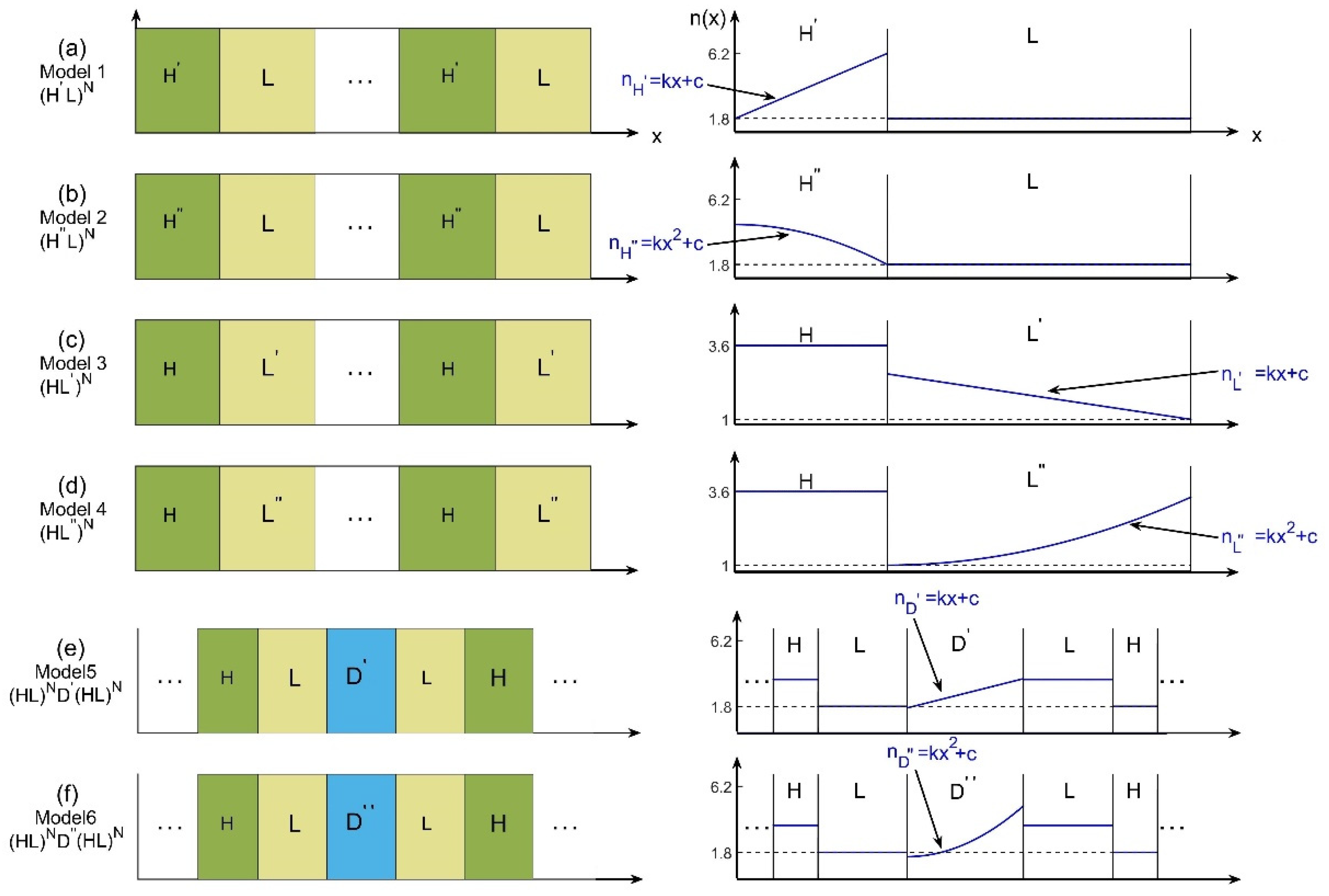
2.1. Physical Model
2.2. Numerical Method
3. Numerical Results and Discussions
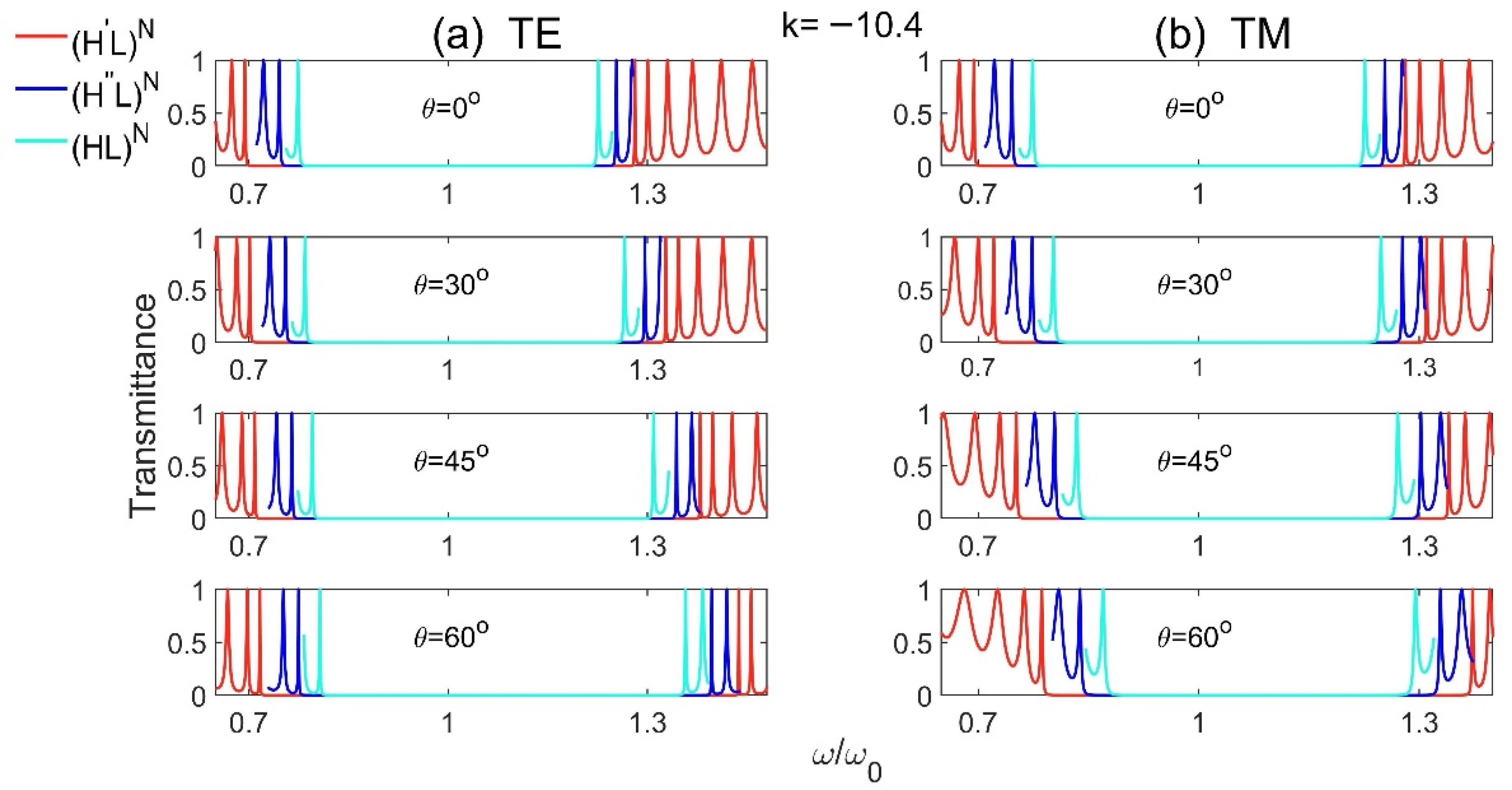
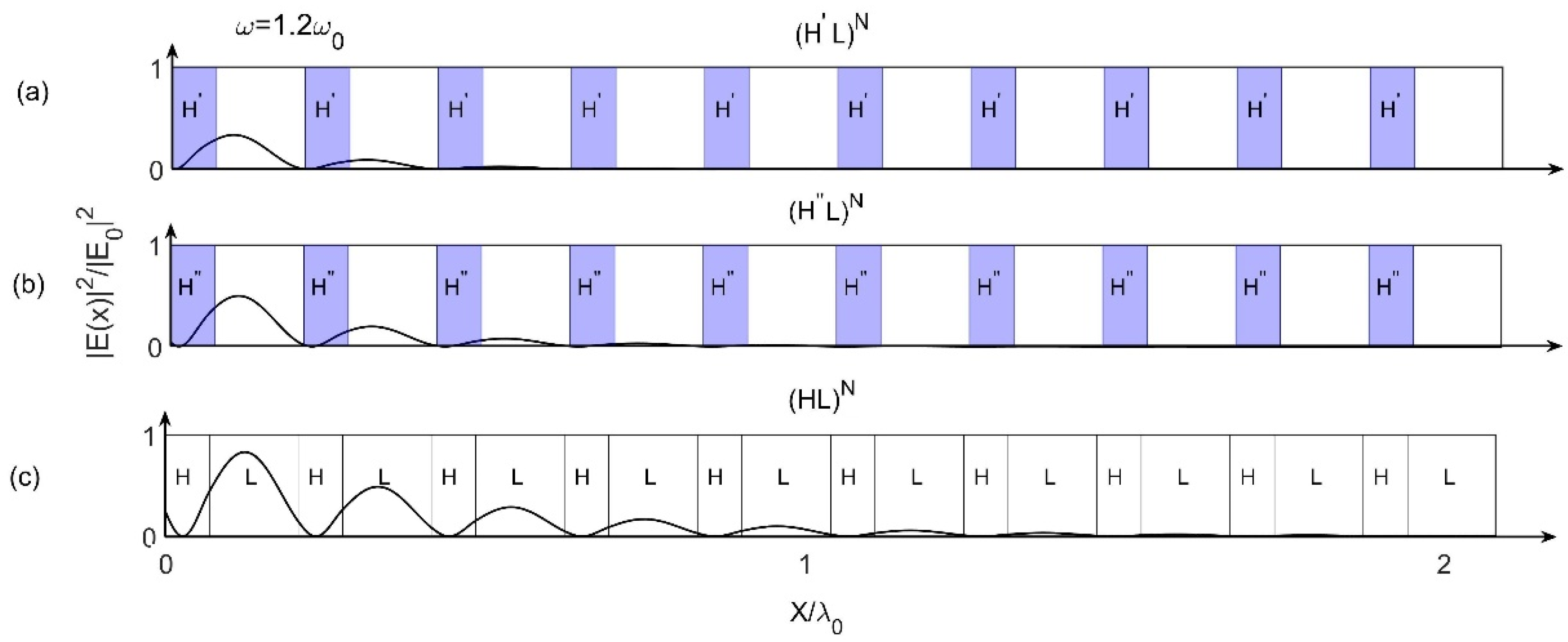
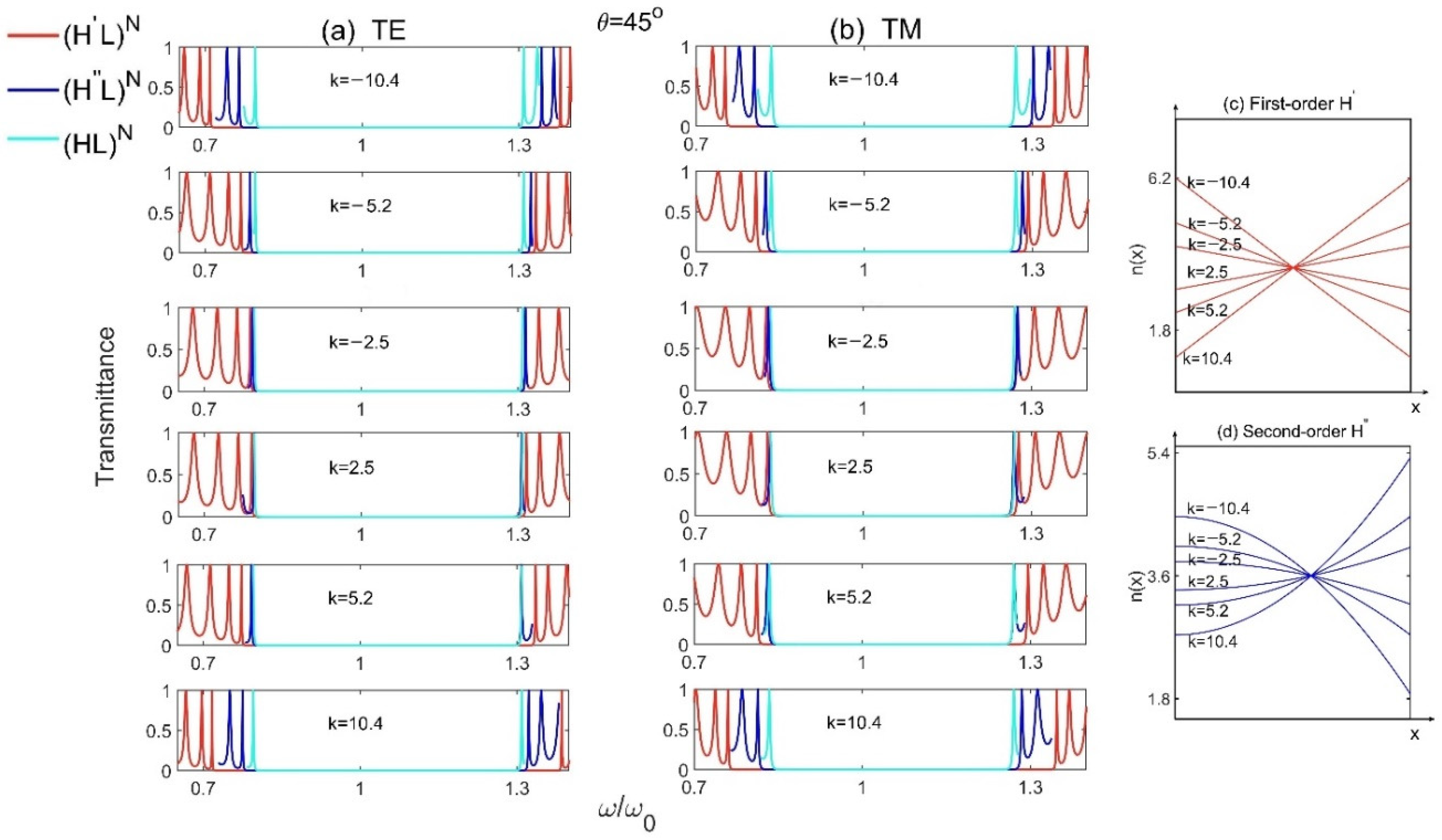
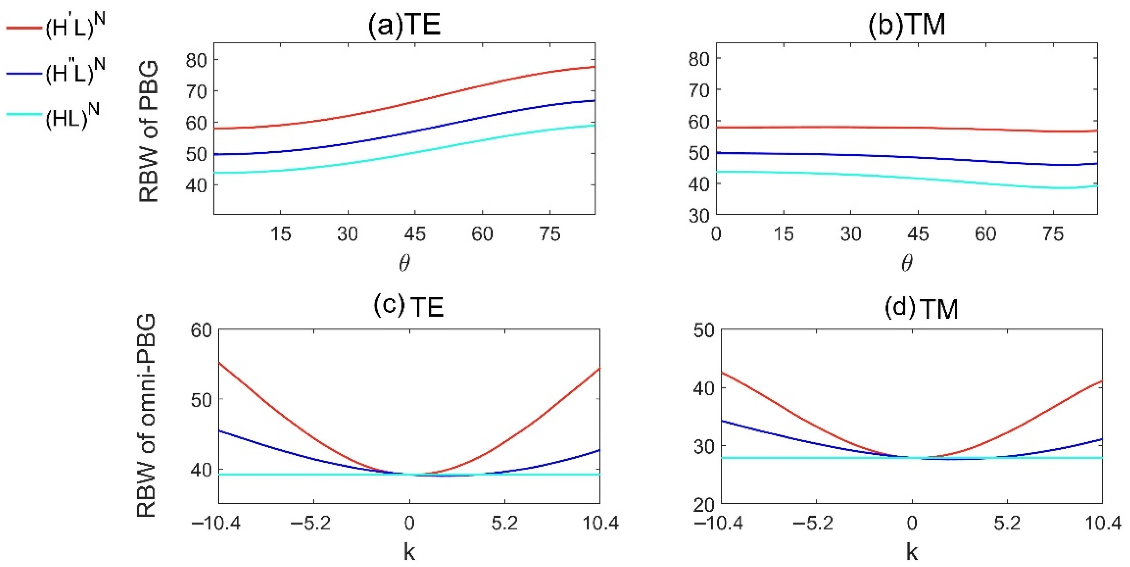
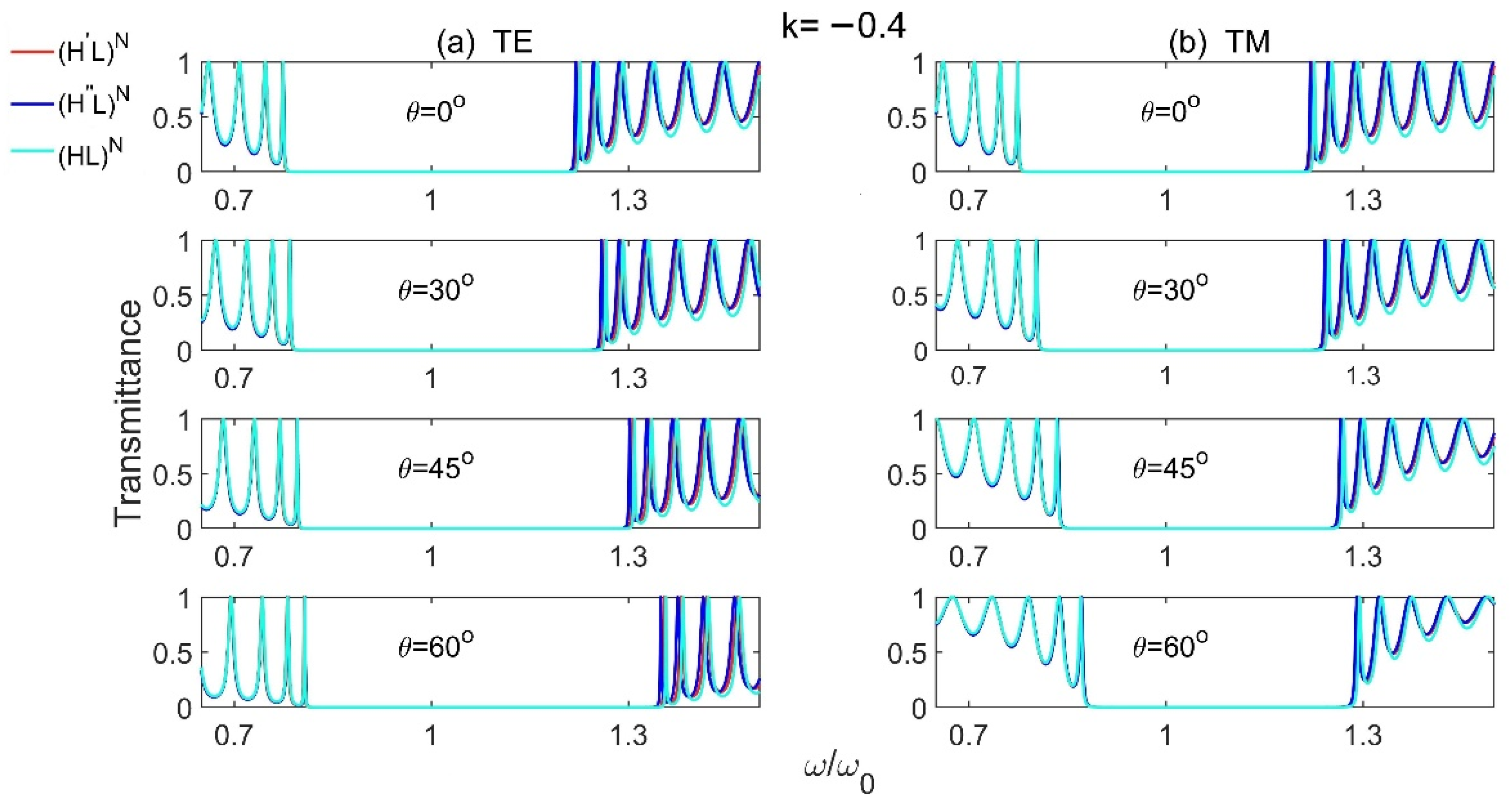
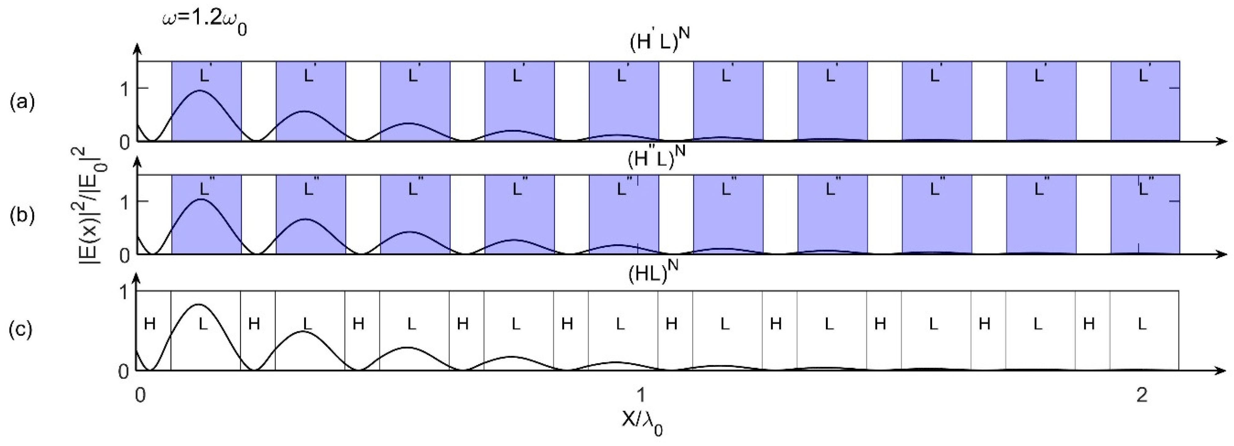
3.1. Research of PBG
3.1.1. PBG Properties of Model 1 and Model 2
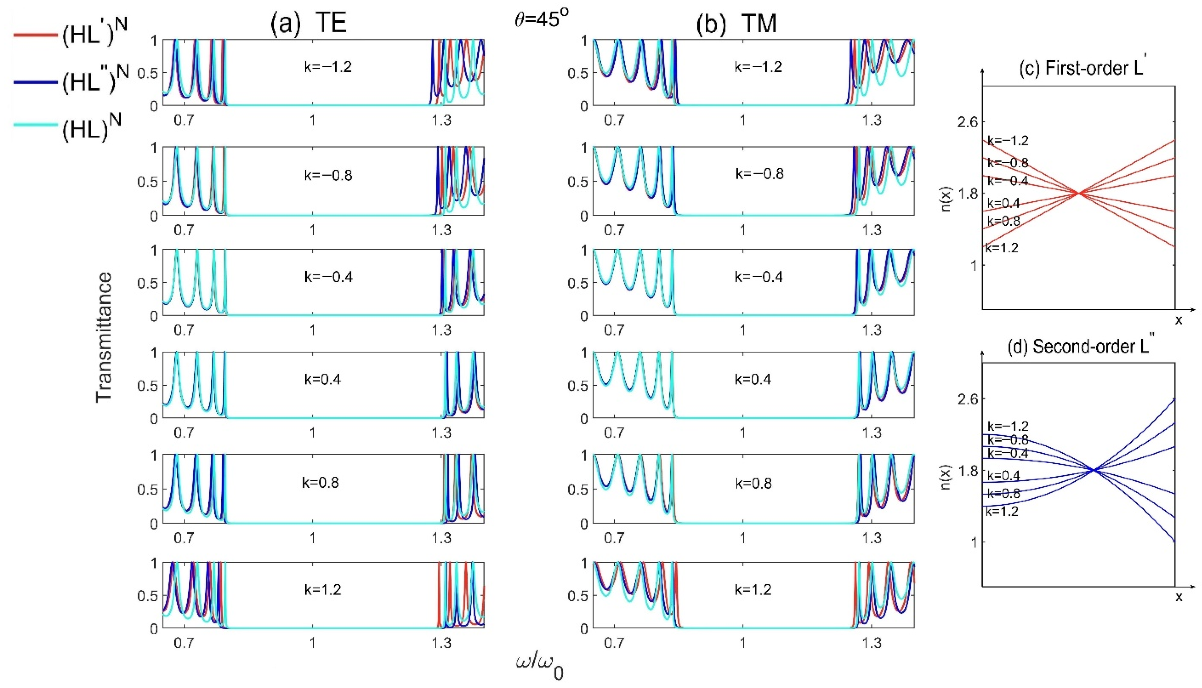
3.1.2. PBG Properties of Model 3 and Model 4
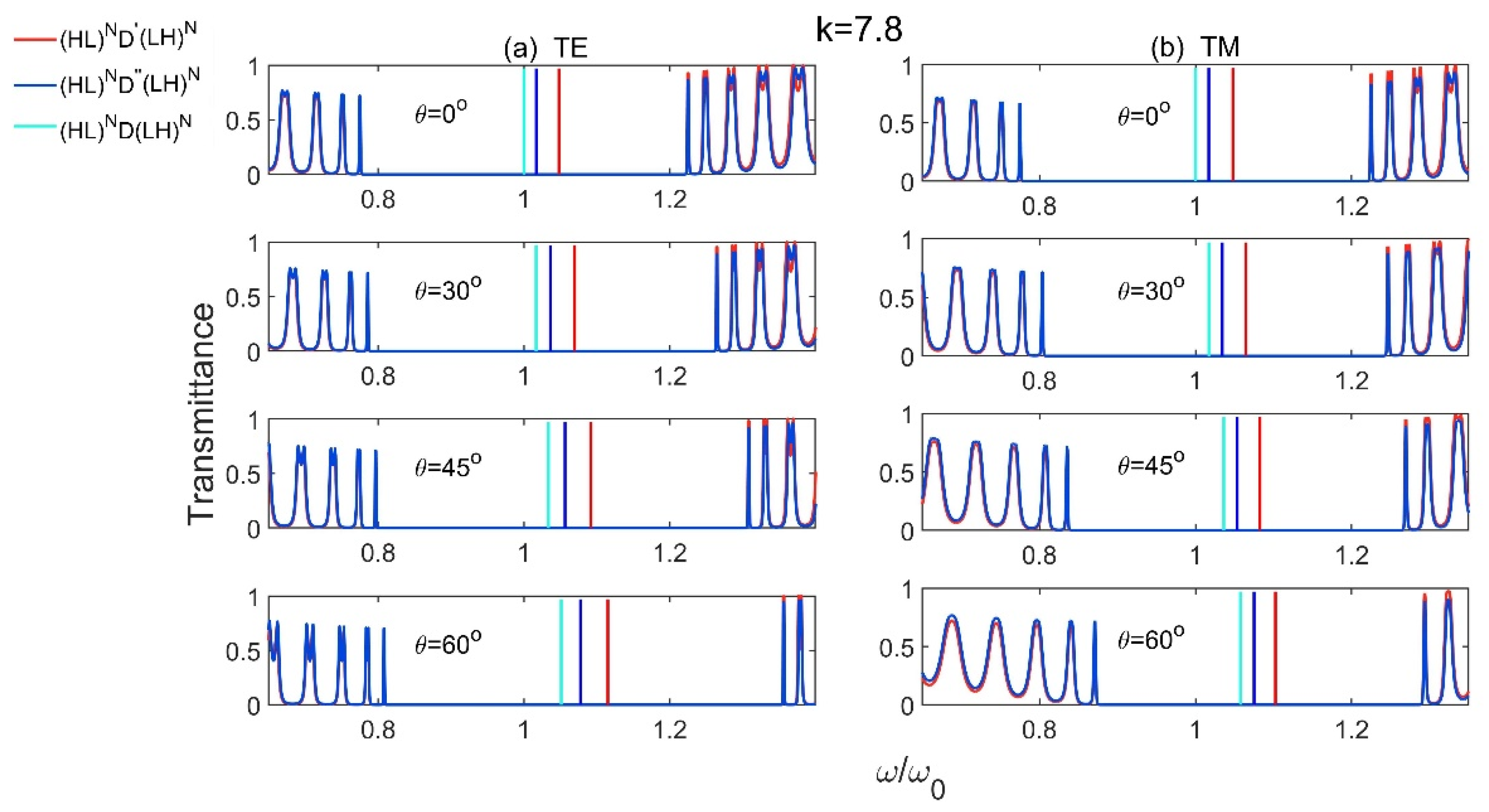
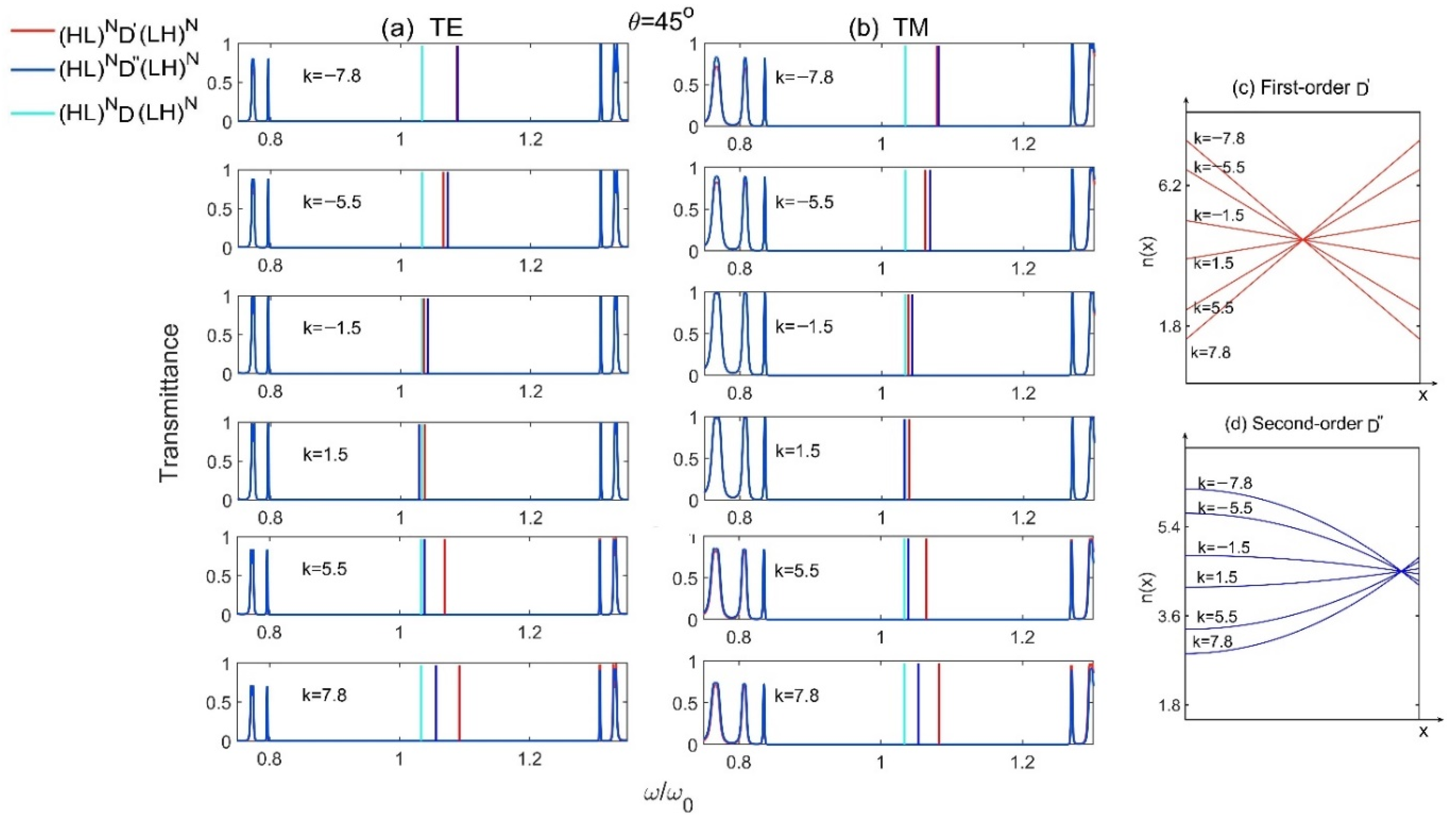
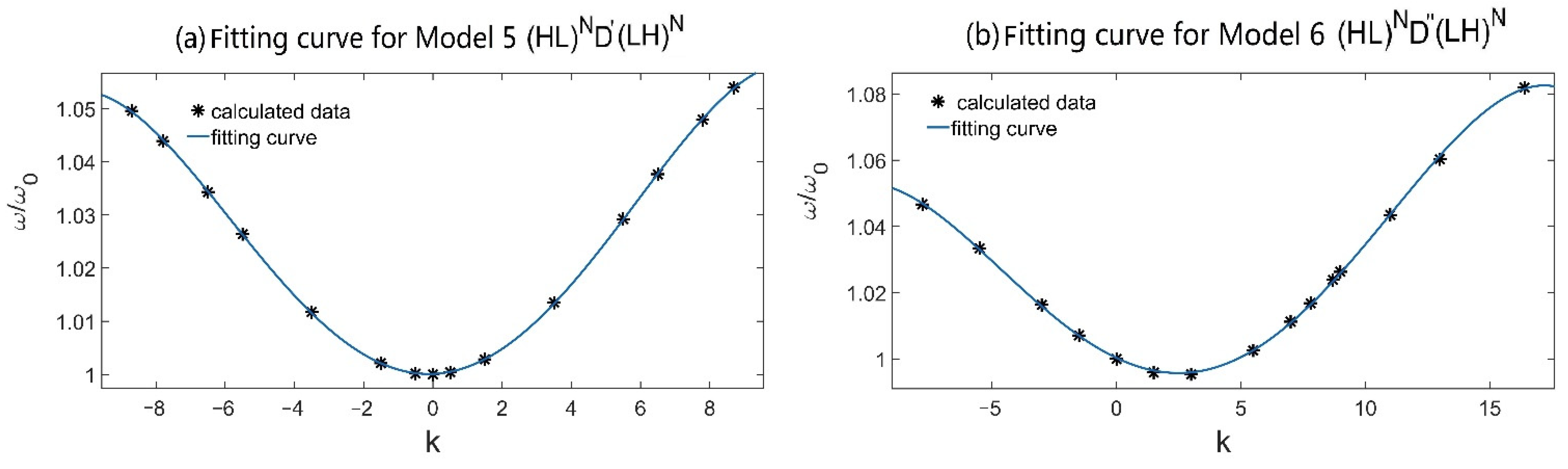
3.2. Research of Defect Mode in Model 5 and Model 6
4. Conclusions
Author Contributions
Funding
Institutional Review Board Statement
Informed Consent Statement
Data Availability Statement
Conflicts of Interest
References
- Yablonovitch, E. Inhibited spontaneous emission in solid-state physics and electronics. Phys. Rev. Lett. 1987, 58, 2059–2062. [Google Scholar] [CrossRef] [PubMed] [Green Version]
- John, S. Strong localization of photons in certain disordered dielectric superlattices. Phys. Rev. Lett. 1987, 58, 2486–2489. [Google Scholar] [CrossRef] [PubMed] [Green Version]
- Joannopoulos, J.D.; Villeneuve, P.R.; Fan, S. Photonic crystals: Putting a new twist on light. Nature 1997, 386, 143–149. [Google Scholar] [CrossRef]
- Thylen, L.; Qiu, M.; Anand, S. Photonic crystals—A step towards integrated circuits for photonics. Chemphyschem 2004, 5, 1268–1283. [Google Scholar] [CrossRef] [PubMed]
- Joannopoulos, J.D.; Johnson, S.G.; Winn, J.N.; Meade, R.D. Photonic Crystals: Molding the Flow of Light, 2nd ed.; Princeton University Press: Princeton, NJ, USA, 2011. [Google Scholar]
- Inoue, K.; Ohtaka, K. Photonic Crystals: Physics, Fabrication and Applications, 1st ed.; Springer Science & Business Media: Berlin/Heidelberg, Germany, 2004. [Google Scholar]
- Kosaka, H.; Kawashima, T.; Tomita, A.; Notomi, M.; Tamamura, T.; Sato, T.; Kawakami, S. Self-collimating phenomena in photonic crystals. Appl. Phys. Lett. 1999, 74, 1212–1214. [Google Scholar] [CrossRef]
- Zalevsky, Z.; George, A.K.; Luan, F.; Bouwmans, G.; Dainese, P.; Cordeiro, C.; July, N. Photonic crystal in-fiber devices. Opt. Eng. 2005, 44, 125003. [Google Scholar] [CrossRef]
- Ayre, M.; Cambournac, C.; Khayam, O.; Benisty, H.; Stomeo, T.; Krauss, T.F. Photonic crystal waveguides for coarse-selectivity devices. Photonics Nanostruct.—Fundam. Appl. 2008, 6, 19–25. [Google Scholar] [CrossRef]
- Zhou, W.; Mackie, D.M.; Taysing-Lara, M.; Dang, G.; Newman, P.G.; Svensson, S. Novel reconfigurable semiconductor photonic crystal-MEMS device. Solid-State Electron. 2006, 50, 908–913. [Google Scholar] [CrossRef]
- Rajan, G.; Callaghan, D.; Semenova, Y.; Farrell, G. Photonic crystal fiber sensors for minimally invasive surgical devices. IEEE Trans. Biomed. Eng. 2012, 59, 332–338. [Google Scholar] [CrossRef]
- Ansari, N.; Tehranchi, M.M.; Ghanaatshoar, M. Characterization of defect modes in one-dimensional photonic crystals: An analytic approach. Phys. B 2009, 404, 1181–1186. [Google Scholar] [CrossRef]
- Kawai, N.K.N.; Wada, M.W.M.; Sakoda, K.S.K. Numerical analysis of localized defect modes in a photonic crystal: Two-dimensional triangular lattice with square rods. Jpn. J. Appl. Phys. 1998, 37, 4644. [Google Scholar] [CrossRef]
- Zhang, L.; Qiao, W.; Chen, L.; Wang, J.; Zhao, Y.; Wang, Q.; He, L. Double defect modes of one-dimensional dielectric photonic crystals containing a single negative material defect. Optik 2014, 125, 1354–1357. [Google Scholar] [CrossRef]
- Yang, D.Q.; Wang, C.; Ji, Y.F. Silicon on-chip 1D photonic crystal nanobeam bandstop filters for the parallel multiplexing of ultra-compact integrated sensor array. Opt. Express 2016, 24, 16267–16279. [Google Scholar] [CrossRef] [PubMed]
- Taha, T.A.; Mehaney, A.; Elsayed, H.A. Detection of heavy metals using one-dimensional gyroidal photonic crystals for effective water treatment. Mater. Chem. Phys. 2022, 285, 126125. [Google Scholar] [CrossRef]
- Alrowaili, Z.A.; Elsayed, H.A.; Ahmed, A.M.; Taha, T.A.; Mehaney, A. Simple, efficient and accurate method toward the monitoring of ethyl butanoate traces. Opt. Quantum Electron 2022, 54, 126. [Google Scholar] [CrossRef] [PubMed]
- Kumar, V.; Singh, K.S.; Ojha, S. Enhanced omni-directional reflection frequency range in Si-based one dimensional photonic crystal with defect. Optik 2011, 122, 910–913. [Google Scholar] [CrossRef]
- Deng, Z.; Su, Y.; Gong, W.; Wang, X.; Gong, R. Temperature characteristics of Ge/ZnS one-dimension photonic crystal for infrared camouflage. Opt. Mater. 2021, 121, 111564. [Google Scholar] [CrossRef]
- Moghadam, R.Z.; Ahmadvand, H. Optical and Mechanical Properties of ZnS/Ge0.1C0.9 Antireflection Coating on Ge Substrate. Iran. J. Sci. Technol. Trans. A Sci. 2021, 45, 1491–1497. [Google Scholar] [CrossRef]
- Zhu, Q.; Jin, L.; Fu, Y. Graded index photonic crystals: A review. Ann. Der Phys. 2015, 527, 205–218. [Google Scholar] [CrossRef]
- Kurt, H.; Citrin, D.S. Graded index photonic crystals. Opt. Express 2007, 15, 1240–1253. [Google Scholar] [CrossRef]
- Singh, B.K.; Chaudhari, M.K.; Pandey, P.C. Photonic and Omnidirectional Band Gap Engineering in One-Dimensional Photonic Crystals Consisting of Linearly Graded Index Material. J. Light. Technol. 2016, 34, 2431–2438. [Google Scholar] [CrossRef]
- Singh, B.K.; Tiwari, S.; Chaudhari, M.K.; Pandey, P.C. Tunable photonic defect modes in one-dimensional photonic crystals containing exponentially and linearly graded index defect. Optik 2016, 127, 6452–6462. [Google Scholar] [CrossRef]
- Singh, B.K.; Bambole, V.; Rastogi, V.; Pandey, P.C. Multi-channel photonic bandgap engineering in hyperbolic graded index materials embedded one-dimensional photonic crystals. Opt. Laser Technol. 2020, 129, 106293. [Google Scholar] [CrossRef]
- Osting, B. Bragg structure and the first spectral gap. Appl. Math. Lett. 2012, 25, 1926–1930. [Google Scholar] [CrossRef] [Green Version]
- Born, M.; Wolf, E. Principles of Optics: Electromagnetic Theory of Propagation, Interference and Diffraction of Light, 7th ed.; Cambridge University Press: Cambridge, UK, 2013. [Google Scholar]
- Al-ghezi, H.; Gnawali, R.; Banerjee, P.P.; Sun, L.; Slagle, J.; Evans, D. 2X2 anisotropic transfer matrix approach for optical propagation in uniaxial transmission filter structures. Opt. Express 2020, 28, 35761–35783. [Google Scholar] [CrossRef] [PubMed]
- Zhang, Y.; Feng, N.; Wang, G.; Zheng, H. Reflection and transmission coefficients in multilayered fully anisotropic media solved by transfer matrix method with plane waves for predicting energy transmission course. IEEE Trans. Antennas Propag. 2021, 69, 4727–4736. [Google Scholar] [CrossRef]
- Giltner, D.M.; McGowan, R.W.; Lee, S.A. Theoretical and experimental study of the Bragg scattering of atoms from a standing light wave. Phys. Rev. A 1995, 52, 3966–3972. [Google Scholar] [CrossRef]
- Nilsen-Hofseth, S.; Romero-Rochin, V. Dispersion relation of guided-mode resonances and Bragg peaks in dielectric diffraction gratings. Phys. Rev. E 2001, 64, 036614. [Google Scholar] [CrossRef]


| TE | TM | ||||||
|---|---|---|---|---|---|---|---|
| 0° | 0.5792 | 0.4958 | 0.4370 | 0.5792 | 0.4958 | 0.4370 | |
| 30° | 0.6192 | 0.5307 | 0.4676 | 0.5796 | 0.4904 | 0.4279 | |
| 45° | 0.6645 | 0.5701 | 0.5020 | 0.5776 | 0.4824 | 0.4155 | |
| 60° | 0.7164 | 0.6152 | 0.5413 | 0.5723 | 0.4705 | 0.3988 | |
| Omni-PBG | 0.5533 | 0.4626 | 0.3992 | 0.4485 | 0.3650 | 0.2986 | |
| C-PBG | 0.4485 | 0.3650 | 0.2986 | The same as TE case | |||
| 0° | 0.4835 | 0.4583 | 0.4370 | 0.4835 | 0.4583 | 0.4370 | |
| 30° | 0.5173 | 0.4904 | 0.4676 | 0.4778 | 0.4505 | 0.4279 | |
| 45° | 0.5554 | 0.5268 | 0.5020 | 0.4694 | 0.4396 | 0.4155 | |
| 60° | 0.5989 | 0.5683 | 0.5413 | 0.4572 | 0.4247 | 0.3988 | |
| Omni-PBG | 0.4500 | 0.4220 | 0.3992 | 0.3532 | 0.3236 | 0.2986 | |
| C-PBG | 0.3532 | 0.3236 | 0.2986 | The same as TE case | |||
| 0° | 0.4491 | 0.4446 | 0.4370 | 0.4491 | 0.4446 | 0.4370 | |
| 30° | 0.4805 | 0.4757 | 0.4676 | 0.4409 | 0.4359 | 0.4279 | |
| 45° | 0.5158 | 0.5109 | 0.5020 | 0.4296 | 0.4240 | 0.4155 | |
| 60° | 0.5562 | 0.5510 | 0.5413 | 0.4140 | 0.4079 | 0.3988 | |
| Omni-PBG | 0.4125 | 0.4074 | 0.3992 | 0.3138 | 0.3078 | 0.2986 | |
| C-PBG | 0.3138 | 0.3078 | 0.2986 | The same as TE case | |||
| 0° | 0.4475 | 0.4352 | 0.4370 | 0.4475 | 0.4352 | 0.4370 | |
| 30° | 0.4788 | 0.4655 | 0.4676 | 0.4392 | 0.4260 | 0.4279 | |
| 45° | 0.5142 | 0.4996 | 0.5020 | 0.4280 | 0.4137 | 0.4155 | |
| 60° | 0.5546 | 0.5386 | 0.5413 | 0.4128 | 0.3972 | 0.3988 | |
| Omni-PBG | 0.4101 | 0.3971 | 0.3992 | 0.3088 | 0.2958 | 0.2986 | |
| C-PBG | 0.3088 | 0.2958 | 0.2986 | The same as TE case | |||
| 0° | 0.4808 | 0.4399 | 0.4370 | 0.4808 | 0.4399 | 0.4370 | |
| 30° | 0.5146 | 0.4705 | 0.4676 | 0.4751 | 0.4313 | 0.4279 | |
| 45° | 0.5528 | 0.5049 | 0.5020 | 0.4668 | 0.4197 | 0.4155 | |
| 60° | 0.5965 | 0.5443 | 0.5413 | 0.4552 | 0.4042 | 0.3988 | |
| Omni-PBG | 0.4460 | 0.4024 | 0.3992 | 0.3445 | 0.3004 | 0.2986 | |
| C-PBG | 0.3445 | 0.3004 | 0.2986 | The same as TE case | |||
| 0° | 0.5762 | 0.4677 | 0.4370 | 0.5762 | 0.4677 | 0.4370 | |
| 30° | 0.6165 | 0.5002 | 0.4676 | 0.5768 | 0.4617 | 0.4279 | |
| 45° | 0.6623 | 0.5368 | 0.5020 | 0.5753 | 0.4532 | 0.4155 | |
| 60° | 0.7148 | 0.5787 | 0.5413 | 0.5706 | 0.4415 | 0.3988 | |
| Omni-PBG | 0.5487 | 0.4327 | 0.3992 | 0.4375 | 0.3310 | 0.2986 | |
| C-PBG | 0.4375 | 0.3310 | 0.2986 | The same as TE case | |||
| TE | TM | ||||||
|---|---|---|---|---|---|---|---|
| 0° | 1.0439 | 1.0466 | 1 | 1.0439 | 1.0466 | 1 | |
| 30° | 1.0650 | 1.0672 | 1.0165 | 1.0603 | 1.0628 | 1.0171 | |
| 45° | 1.0869 | 1.0884 | 1.0335 | 1.0783 | 1.0805 | 1.0361 | |
| 60° | 1.1095 | 1.1102 | 1.0510 | 1.0982 | 1.1003 | 1.0576 | |
| 0° | 1.0264 | 1.0334 | 1 | 1.0264 | 1.0334 | 1 | |
| 30° | 1.0458 | 1.0528 | 1.0165 | 1.0432 | 1.0500 | 1.0171 | |
| 45° | 1.0658 | 1.0729 | 1.0335 | 1.0617 | 1.0683 | 1.0361 | |
| 60° | 1.0866 | 1.0937 | 1.0510 | 1.0824 | 1.0887 | 1.0576 | |
| 0° | 1.0021 | 1.0071 | 1 | 1.0021 | 1.0071 | 1 | |
| 30° | 1.0189 | 1.0242 | 1.0165 | 1.0192 | 1.0241 | 1.0171 | |
| 45° | 1.0361 | 1.0418 | 1.0335 | 1.0382 | 1.0430 | 1.0361 | |
| 60° | 1.0539 | 1.0599 | 1.0510 | 1.0596 | 1.0643 | 1.0576 | |
| 0° | 1.0028 | 0.9959 | 1 | 1.0028 | 0.9959 | 1 | |
| 30° | 1.0197 | 1.0122 | 1.0165 | 1.0199 | 1.0131 | 1.0171 | |
| 45° | 1.0370 | 1.0290 | 1.0335 | 1.0389 | 1.0322 | 1.0361 | |
| 60° | 1.0548 | 1.0463 | 1.0510 | 1.0603 | 1.0538 | 1.0576 | |
| 0° | 1.0292 | 1.0026 | 1 | 1.0292 | 1.0026 | 1 | |
| 30° | 1.0489 | 1.0201 | 1.0165 | 1.0461 | 1.0200 | 1.0171 | |
| 45° | 1.0692 | 1.0383 | 1.0335 | 1.0647 | 1.0392 | 1.0361 | |
| 60° | 1.0903 | 1.0571 | 1.0510 | 1.0854 | 1.0608 | 1.0576 | |
| 0° | 1.0479 | 1.0169 | 1 | 1.0479 | 1.0169 | 1 | |
| 30° | 1.0694 | 1.0362 | 1.0165 | 1.0644 | 1.0343 | 1.0171 | |
| 45° | 1.0918 | 1.0564 | 1.0335 | 1.0825 | 1.0536 | 1.0361 | |
| 60° | 1.1149 | 1.0774 | 1.0510 | 1.1025 | 1.0750 | 1.0576 | |
Publisher’s Note: MDPI stays neutral with regard to jurisdictional claims in published maps and institutional affiliations. |
© 2022 by the authors. Licensee MDPI, Basel, Switzerland. This article is an open access article distributed under the terms and conditions of the Creative Commons Attribution (CC BY) license (https://creativecommons.org/licenses/by/4.0/).
Share and Cite
Fu, L.; Lin, M.; Liang, Z.; Wang, Q.; Zheng, Y.; Ouyang, Z. The Transmission Properties of One-Dimensional Photonic Crystals with Gradient Materials. Materials 2022, 15, 8049. https://doi.org/10.3390/ma15228049
Fu L, Lin M, Liang Z, Wang Q, Zheng Y, Ouyang Z. The Transmission Properties of One-Dimensional Photonic Crystals with Gradient Materials. Materials. 2022; 15(22):8049. https://doi.org/10.3390/ma15228049
Chicago/Turabian StyleFu, Lixin, Mi Lin, Zixian Liang, Qiong Wang, Yaoxian Zheng, and Zhengbiao Ouyang. 2022. "The Transmission Properties of One-Dimensional Photonic Crystals with Gradient Materials" Materials 15, no. 22: 8049. https://doi.org/10.3390/ma15228049