2.1. Analytical Model for Buckling of a Column with Pin Connections at Ends with Stepwise Variable Section
In
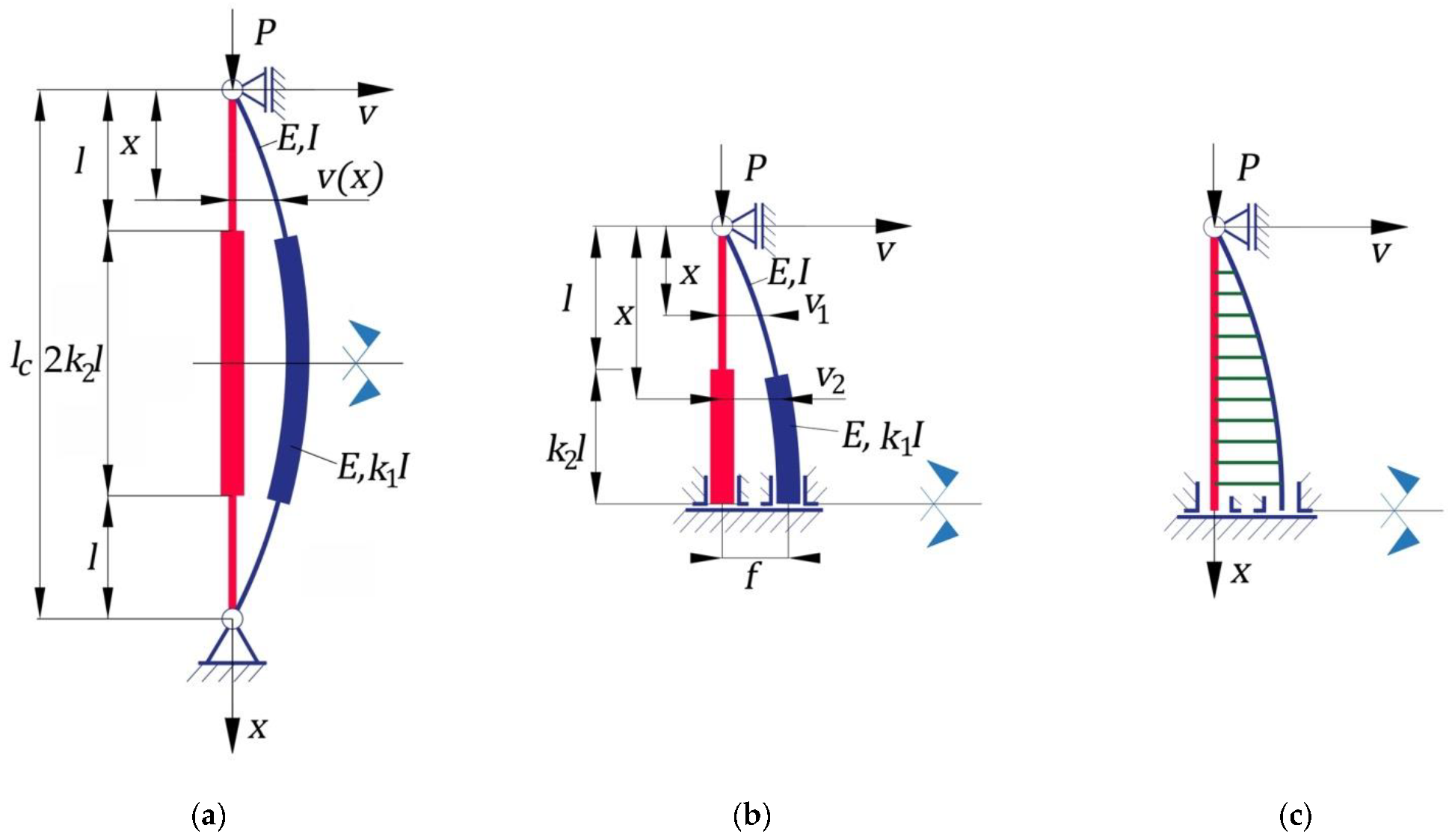
Figure 1, a geometrical model is shown of a bar having a stepwise variable circular cross-section whose bottom end is pin-connected, while the upper end is simply supported. The undeformed and deformed shapes of the bar under compression are shown in
Figure 1a. The bar consists in three portions. The first and the third portions have the same values for length
and for the second moment of inertia
of the cross-section. The second bar portion has a cross-section whose moment of inertia
is equal to
, with
, and its length is equal to
. In other words, the parameters
and
represent the ratios of the lengths and of the second moment of inertia, respectively, corresponding to the second and first portions of the bar (
Figure 1a). The total length of the column is denoted with
(
Figure 1a). All portions of the bar are made of the same isotropic material having a modulus of elasticity
. The column is symmetric with respect to its midpoint (
Figure 1a), and consequently, the analysis model may be reduced to half of the bar, considering the symmetry conditions (
Figure 1b). The shape of the bending-moment diagram for half of the bar is shown in
Figure 1c.
The main purpose of this subsection is to compare the critical buckling force corresponding to a column having a stepwise variable circular cross-section with the critical buckling force corresponding to a column having the same length and a constant cross-section whose moment of inertia is equal to . For this purpose, the main objectives are to compute the critical buckling force corresponding to the column having a stepwise variable cross-section and to compare it with the one corresponding to the column with a constant cross-section, as well as an analysis of the rational shapes for buckling in the case of columns having stepwise variable circular cross-sections.
Due to symmetry, the buckling analysis was made by considering a model of half of a column (
Figure 1b) with boundary conditions corresponding to the midpoint of the column located on the horizontal symmetry axis.
It was assumed that the column buckled in the elastic domain. This meant that Bernoulli’s hypothesis and Euler’s relation were valid at buckling.
The bending moment
developed at buckling and caused by the compressive force
P at the level of the arbitrary cross-section located on the first portion of the column was computed using Equation (1):
where
represents the deflection function of the arbitrary cross-section of the first column portion located at distance
with respect to the end of the column (
Figure 1b).
In the same manner, the bending moment
developed at buckling at the level of the arbitrary cross-section located on the second portion of the column was computed using Equation (2):
where
represents the deflection function of the arbitrary cross-section of the second column portion located at distance
with respect to the end of the column (
Figure 1b).
To compute the critical buckling force, we used an analytical method. The differential equation of the approximate deformed median fiber corresponding to the first portion of the bar is given in Equation (3):
Replacing Equation (1), Equation (3) became the following [
2]:
In the same manner, the differential equation of the approximate deformed median fiber corresponding to the second portion of the bar is given in Equation (5) [
2]:
The notation
was introduced for the ratio given in Equation (6) [
2]:
By using Equation (6), differential Equations (4) and (5) of the approximate deformed median fibers for the bar portions became:
- 1.
Equation (7) for the first portion of the column [
2]:
- 2.
Equation (8) for the second portion of the column [
2]:
Solutions of inhomogeneous second-order differential Equations (7) and (8) were given by Equations (9) and (10) for the first portion and for the second portion of the column, respectively:
Integration constants
were computed using the boundary conditions given in Equation (11):
where
represents the deflection of the midpoint of the bar at buckling. The continuity conditions for the deformed shape of the median fiber of the column are given in Equation (12) at the level of the bar cross-section located at distance
with respect to the upper simply supported end of the column:
The first derivatives of the functions
and
of the deflections of the arbitrary cross-section corresponding to each column portion were computed using Equations (9) and (10), respectively. In fact, these derivatives represented the functions of the rotations of the arbitrary cross-section and were expressed by Equations (13) and (14):
By replacing Equations (9), (10), (13), and (14) in the boundary conditions given by Equation (11) and in the continuity conditions given in Equation (12), the system of Equation (15) was obtained:
whose unknown quantities are the integration constants
and the deflection
f of the midpoint of the column.
Equation system (15) was reduced practically to the following system of four equations:
The homogeneous system of Equation (16) had nonzero solutions for
and
f if the determinant of the coefficients was zero. This condition led to Equation (17):
The notation
was introduced and computed with Equation (18):
and Equation (17) became:
whose unknown is
ξ. To compute the critical buckling force, the minimum value of the absolute values of the solutions
ξ must be used because, for other solutions
ξ, the value of the critical force would be greater.
denoted the minimum value of the absolute values of the solutions ξ of Equation (19).
From Equation (18), the minimum value of
could be computed using Equation (20):
Equation (20) was replaced in relation (6) in order to compute the critical buckling force for a column having a stepwise variable cross-section:
The length
of the first portion was expressed in the function of the total length
of the column using Equation (22) according to
Figure 1a:
Equation (22) was replaced in Equation (21) in order to compute the critical buckling force
for a column having a stepwise variable cross-section:
On the other hand, the critical buckling force
for a column with a constant cross-section whose moment of inertia of the section was
having the same total length
with pin connections at its ends was computed as follows:
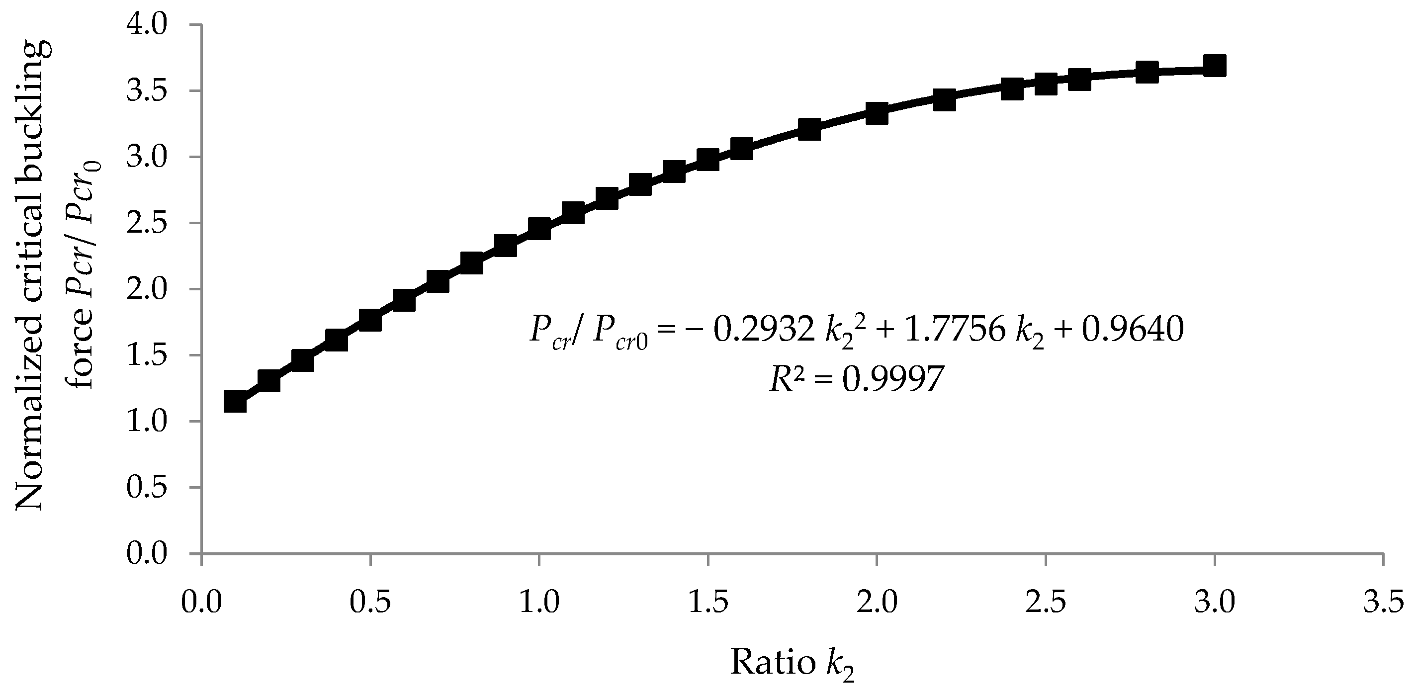
Using Equations (23) and (24), the normalized buckling force (denoted with
c) was computed as being equal with the ratio between the critical buckling force
for a column having a stepwise variable cross-section and the critical buckling force
for a column having a constant cross-section whose moment of inertia of the section was
:
It is said that a column is rationally designed if the critical buckling force is increased while the mass of the material of the column is optimal. In structure design, both the mass of the material, which influences the material costs, and the weight of the structure are also important. The manufacturing costs increase due to the additional manufacturing operations required for a column having a stepwise variable cross-section.
In this research, it was said that a column having a stepwise variable cross-section was rationally designed if its ratio between the critical buckling force and the total volume of the column was greater than the similar ratio computed for a column with a constant cross-section whose moment of inertia of the section was with the same total length .
The ratio between the critical buckling force
and the total volume
of the column was computed as follows, taking into account the geometry of the column shown in
Figure 1a:
where
represents the cross-sectional areas for the first and the third portions of the column having the length
, while
represents the area of the cross-section for the second column portion whose length is equal to
.
It was assumed that each portion of the column had a circular cross-section. It may be remarked in Equation (27), which gives the ratio between the moment of inertia
and the second power of the area of the cross-section
for the first portion, whose diameter is denoted with
:
or
In the same manner, Equation (29) was written for the second portion of the column:
On the other hand, the relation between the moments of inertia
I1 and
I corresponding to the first two portions of the column, respectively, is given in Equation (30):
Equations (28) and (29) were replaced in Equation (30), and it obtained Equation (31):
Then, relations (22) and (31) were replaced in relation (26), which became:
From Equation (25), the critical buckling force
for a column having a stepwise variable cross-section could be computed in the function of the critical buckling force
of a column with a constant cross-section:
The volume of the column with a constant cross-section was:
Replacing Equations (33) and (34) in Equation (32) obtained Equation (35):
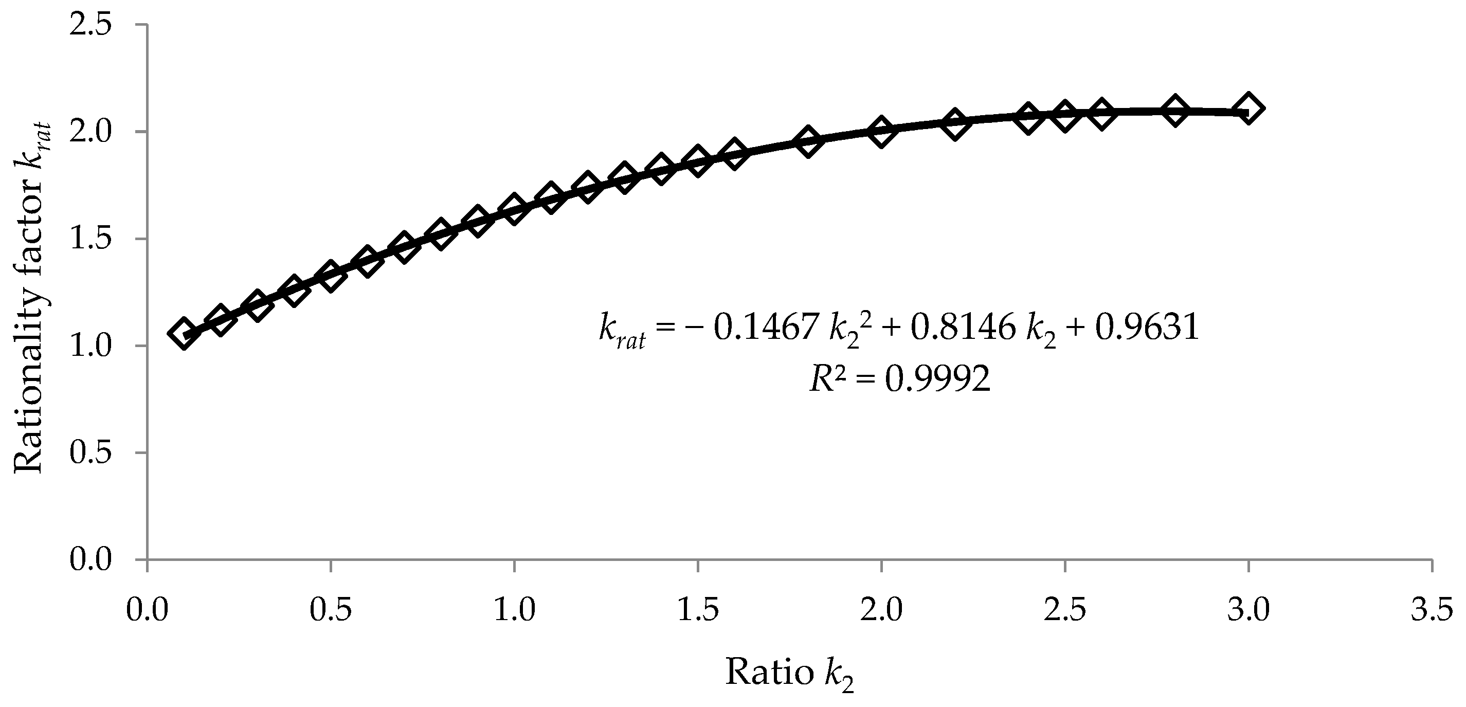
which led to Equation (36), which computed the rationality factor
:
Replacing the ratio
c given by Equation (25) in Equation (36) led to Equation (37):
which was used to compute the ratio between the rationality factor
corresponding to a column having a stepwise variable cross-section and the rationality factor
corresponding to a column with a constant cross-section.
2.2. Numerical Modeling and Simulation for Loss in Stability of a Column with Pin Connections at Ends with Stepwise Variable Cross-Section
If the compressive stress, which acts on the slenderness of a column, is variable, then the relation between force and displacement may be written with Equation (38):
where infinitesimal variation in the force is denoted with
. A similar relation may be written with Equation (39):
where finite variation in the force is denoted with
. In Equations (38) and (39),
and
represent the tangent stiffness matrix and the secant stiffness matrix, respectively. The finite variation in the displacements was computed with Equation (40):
where
is the adjunct matrix of the stiffness matrix.
The phenomenon of loss in stability (transition from one equilibrium shape to another equilibrium shape) takes place when the displacements tend toward infinity for a variation
in the compressive force. From a mathematical point of view, this condition is fulfilled if the determinant of the tangent stiffness matrix
is equal to zero, which was expressed by Equation (41):
Equation (41) could be written with Equation (42):
where
represents the elastic stiffness matrix of the structure (e.g., the column) obtained by assembling of the stiffness matrices
corresponding to the finite elements that form the structure;
is the geometric stiffness matrix of the structure obtained by assembling of the geometric stiffness matrices
corresponding to the finite elements that form the structure; and
is the common multiplier of the axial forces
N acting in the slender bar.
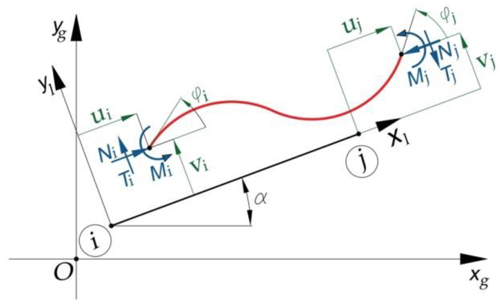
For the finite element of the double-embedded bar type (
Figure 2), the elastic stiffness matrix
and the geometric stiffness matrix
were expressed with Equations (43) and (44), respectively:
where
,
, and
are the length, area of the cross-section, and the second moment of inertia of the cross-section, respectively, corresponding to the finite elements double-embedded at both ends.
In this context, the solving of the stability equation involved solving a problem of eigenvectors and eigenvalues. The solutions of the stability equation were the eigenvalues corresponding to the multiplier of the axial forces. For the eigenvalues , the corresponding eigenvectors were determined, which represented the geometric shapes (equilibrium shapes) of the loss in stability. From a practical point of view, only the lowest eigenvalue was of interest, the other values being of interest just from a theoretical point of view.
The numerical model for the calculation of the critical buckling force was validated for a bar having a pin connection at one end and a simple support at the other end. Considering the numerical model previously described, a computer calculation program was written with MATLAB R2014a software for the calculation of the eigenvalues and eigenvectors for the loss in stability of a slender bar subjected to compression. Because just the first value of the critical buckling force and the corresponding deformed shape were of interest, the calculation program reported just the first three values of the critical buckling force and plotted the corresponding eigenvectors.
The assumptions considered in the numerical analysis of the finite elements were the following: (i) the material of the bar was isotropic, homogeneous, and linearly elastic; (ii) the hypothesis of small strains was valid; and (iii) the normal stress at the proportionality limit was approximately equal to the normal stress at yielding, denoted with , for the material of the bar.
In order to obtain the numerical solution with the finite element method, the main steps covered by the MATLAB program were the following: (i) meshing of the bar in a certain number of finite elements; (ii) computing both the elastic stiffness matrix and the geometric stiffness matrix corresponding to each finite element according to Equations (43) and (44), respectively; (iii) assembling all the stiffness matrices and geometric stiffness matrices in order to obtain the elastic stiffness matrix and geometric stiffness matrix of the column analyzed; (iv) computing the eigenvalues by solving Equation (42); (v) computing the eigenvectors using Equation (40); and (vi) by using the eigenvalues , computing the critical buckling forces . The smallest critical buckling force corresponded to the minimum eigenvalue .
In order to validate the numerical model, the loss in stability was analyzed using the numerical model with 18 finite elements for a bar having a pin connection at one end and a simple support at the other end, for which the geometrical characteristics and the material properties are given in
Table 1. Considering the geometrical characteristics of the bar given in
Table 1, the following quantities were computed: the area
of the cross-section of 2826 mm
2; the second moment of inertia
I of the cross-section, whose value was 2,896,650 mm
4; and the radius
of inertia, having a value of 32.01562 mm.
For the bar involved, the slenderness ratio
was computed with Equation (45):
For steel of type S355, whose properties are shown in
Table 1, the slenderness ratio
that limited buckling in the elastic field was computed with Equation (46):
where it is assumed that the normal stress
at the proportionality limit is approximately equal to the normal stress at yielding, denoted with
, for the material of the bar (
Table 1).
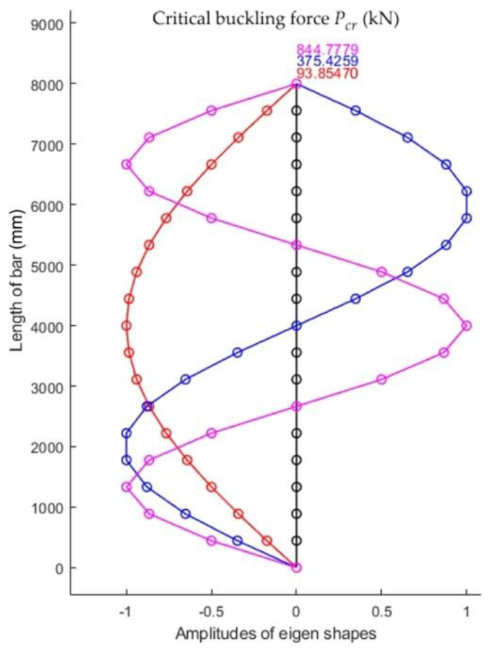
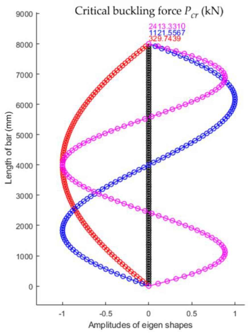
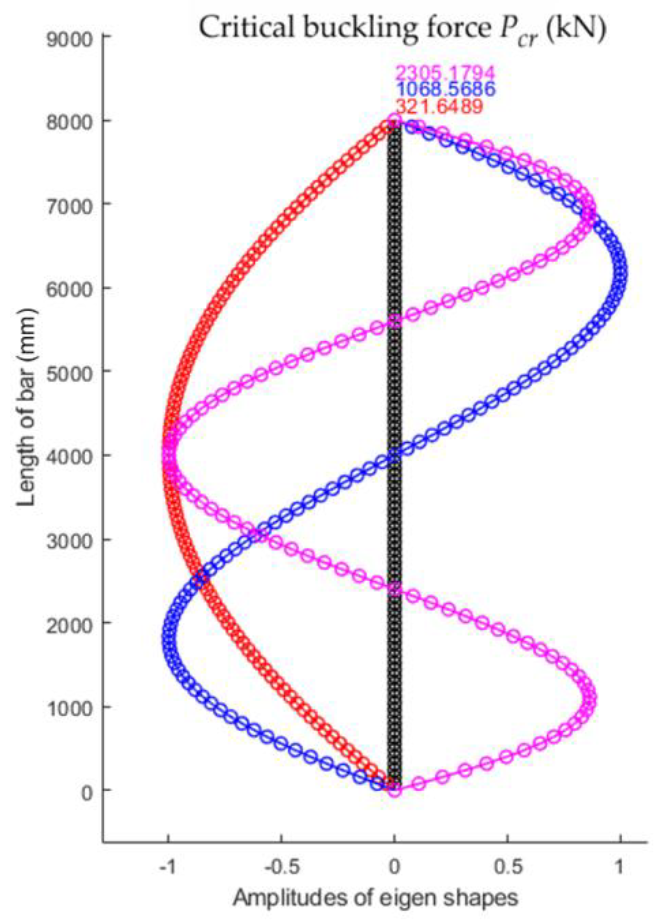
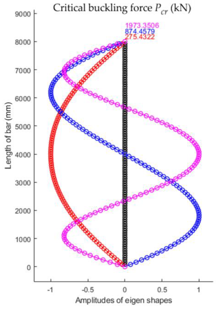
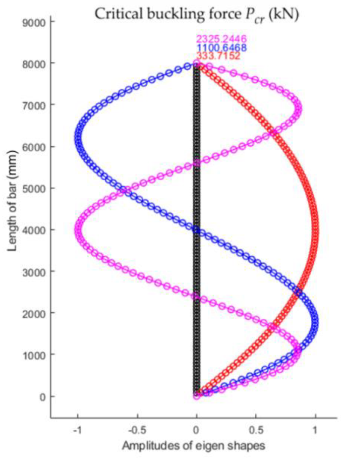
The first three eigenshapes and the corresponding eigenvalues for the bar analyzed are shown in
Figure 3.
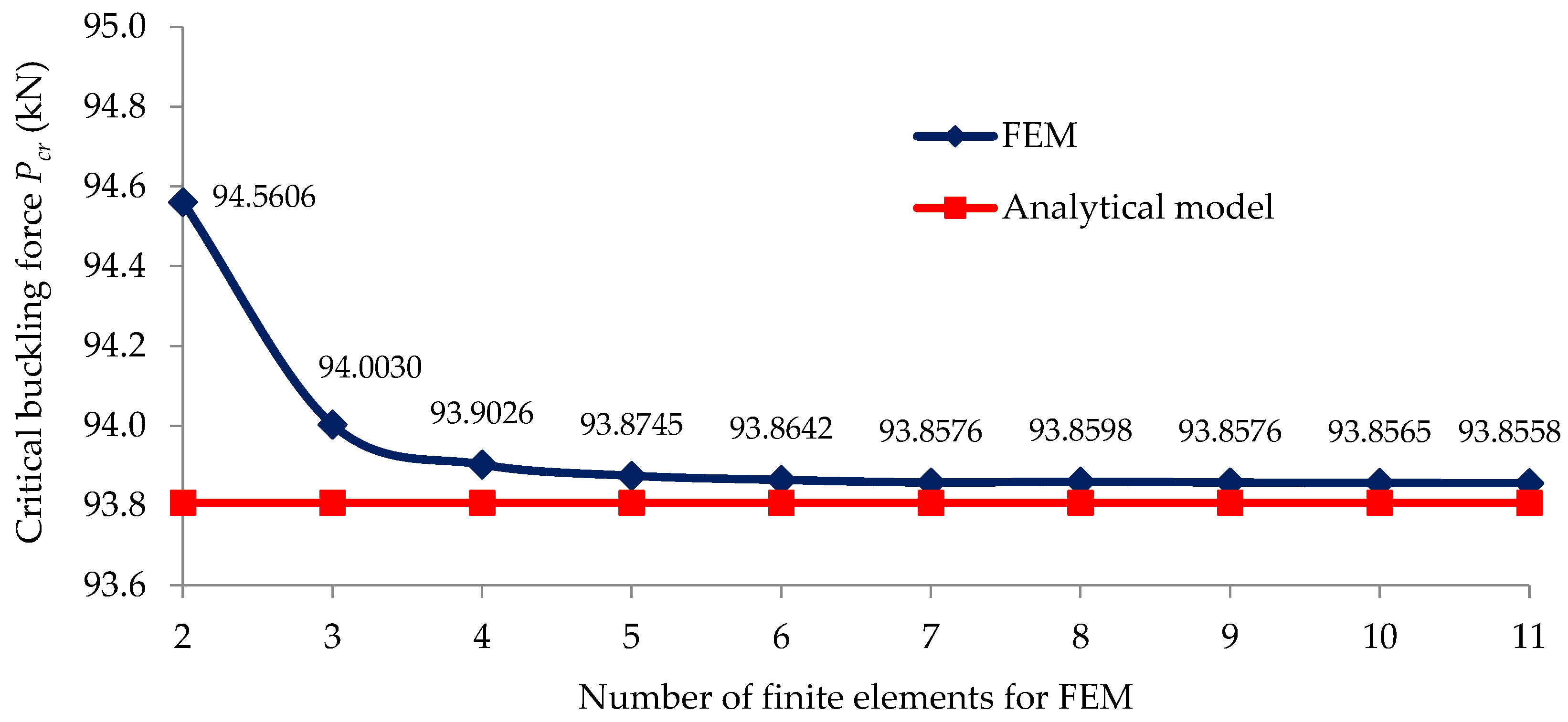
In
Figure 4, the convergence of the critical buckling load
obtained with the algorithm of the numerical model is shown related to the number of the finite elements of the numerical model, and it is analyzed with respect to the critical buckling load of 93.807 kN computed with Equation (24) using the analytical model. By analyzing
Figure 4, it can be remarked that the solutions obtained through numerical modeling with the FEM tended asymptotically to the value of 93.86 kN for the numerical model, which had at least six elements. It can be concluded that the numerical model consisting of 18 finite elements provided results that were sufficiently accurate concerning the critical buckling load.
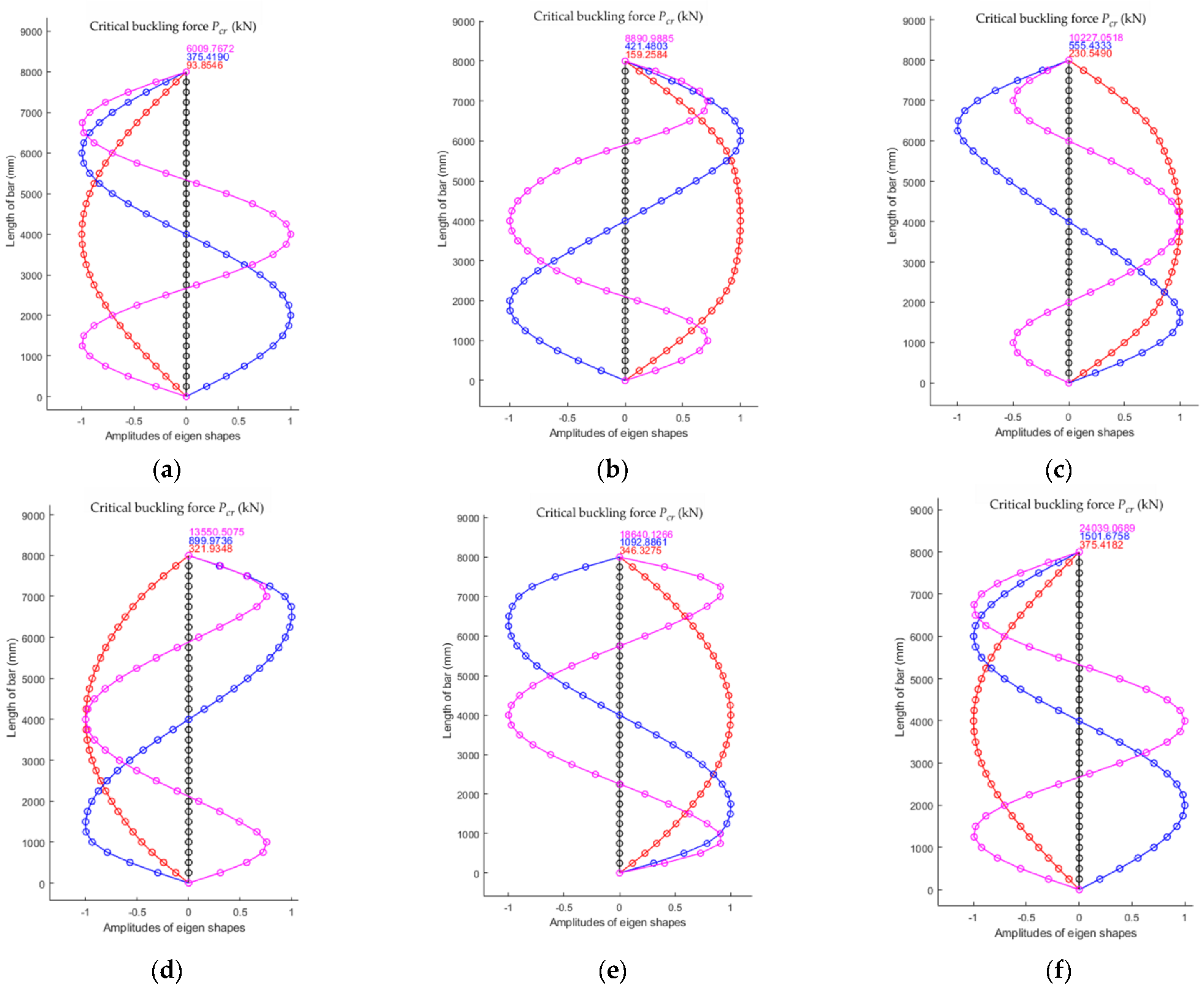
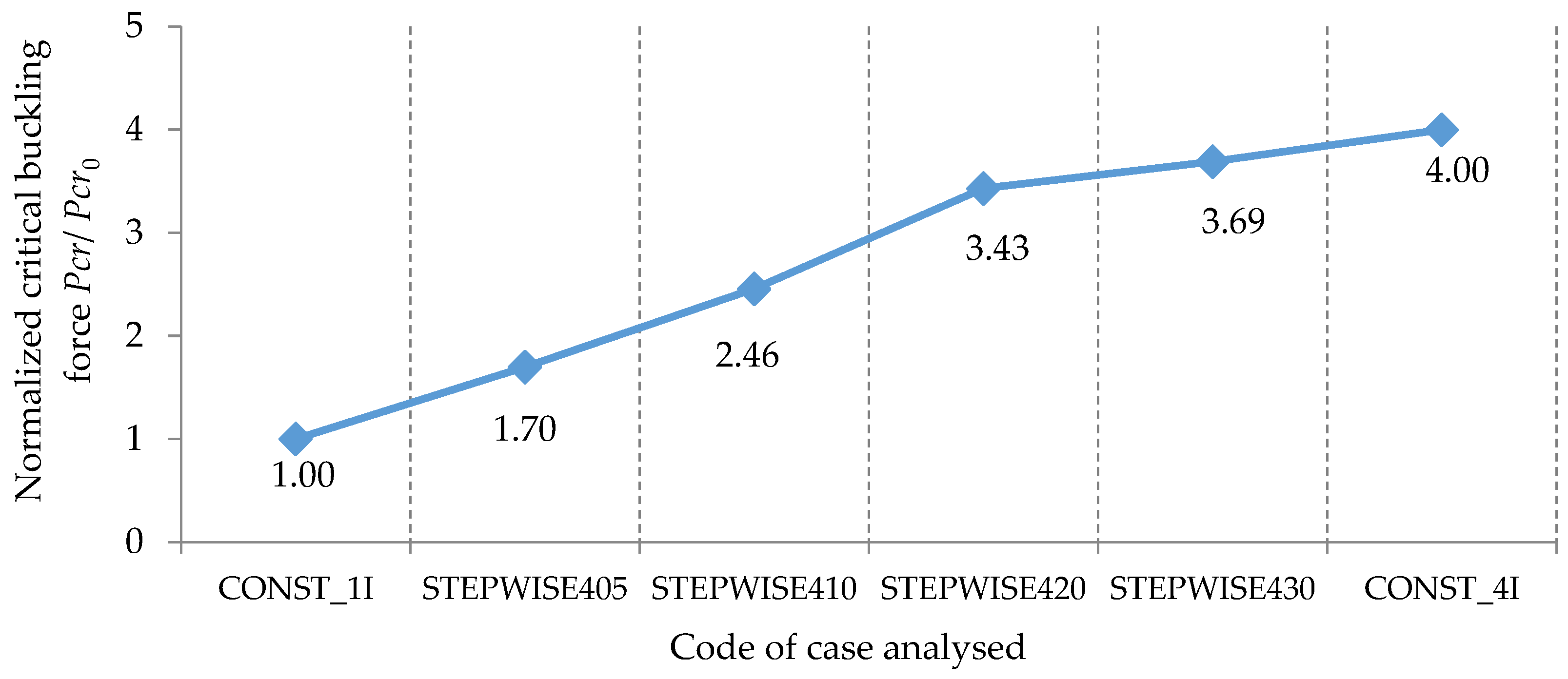
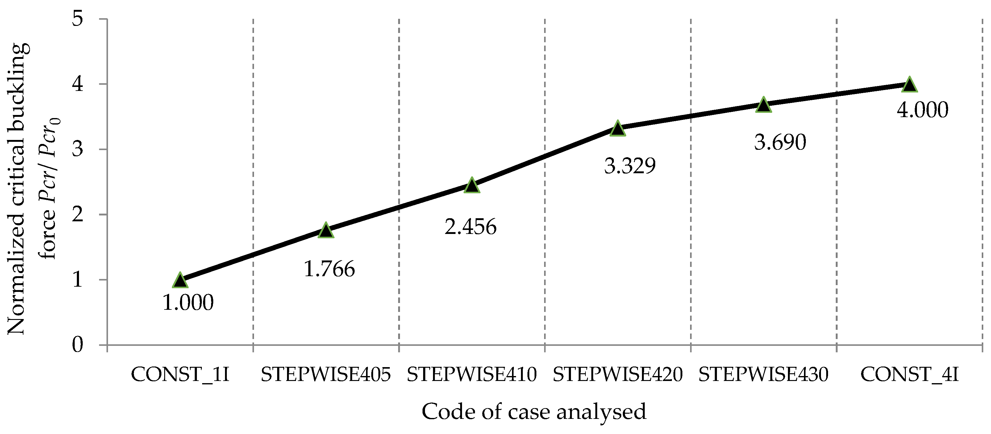
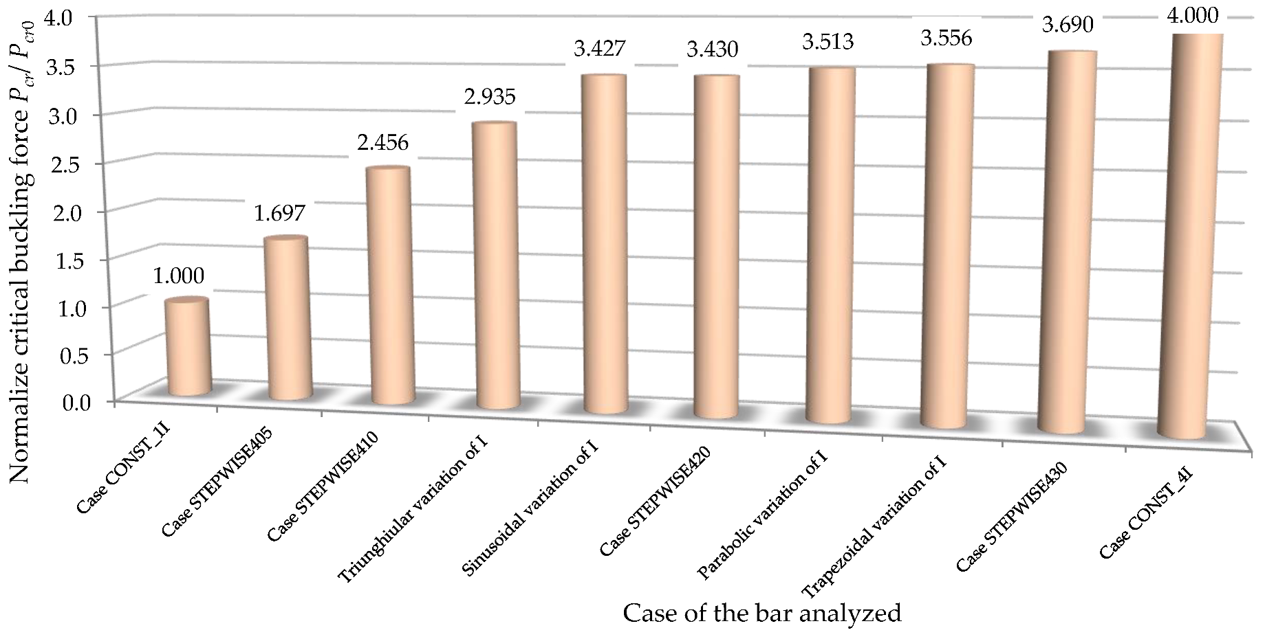
Six cases of bars with pin connections at one end and simple supports at the other end, shown in
Table 2, were analyzed using the numerical model with finite elements in order to show the effects of a stepwise variable cross-section on the critical force of stability loss.
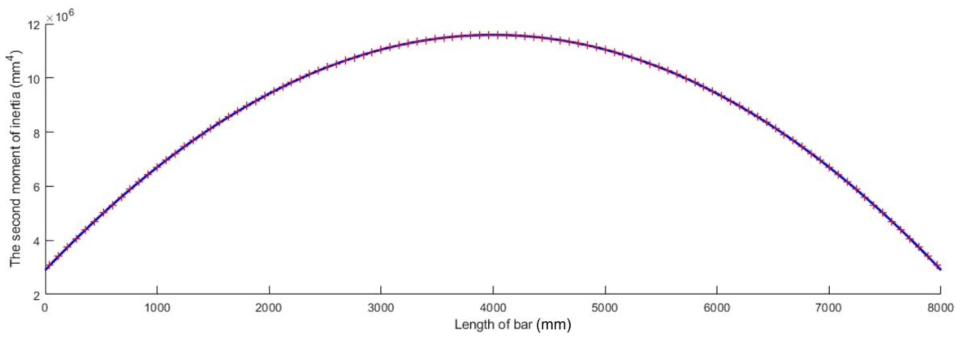
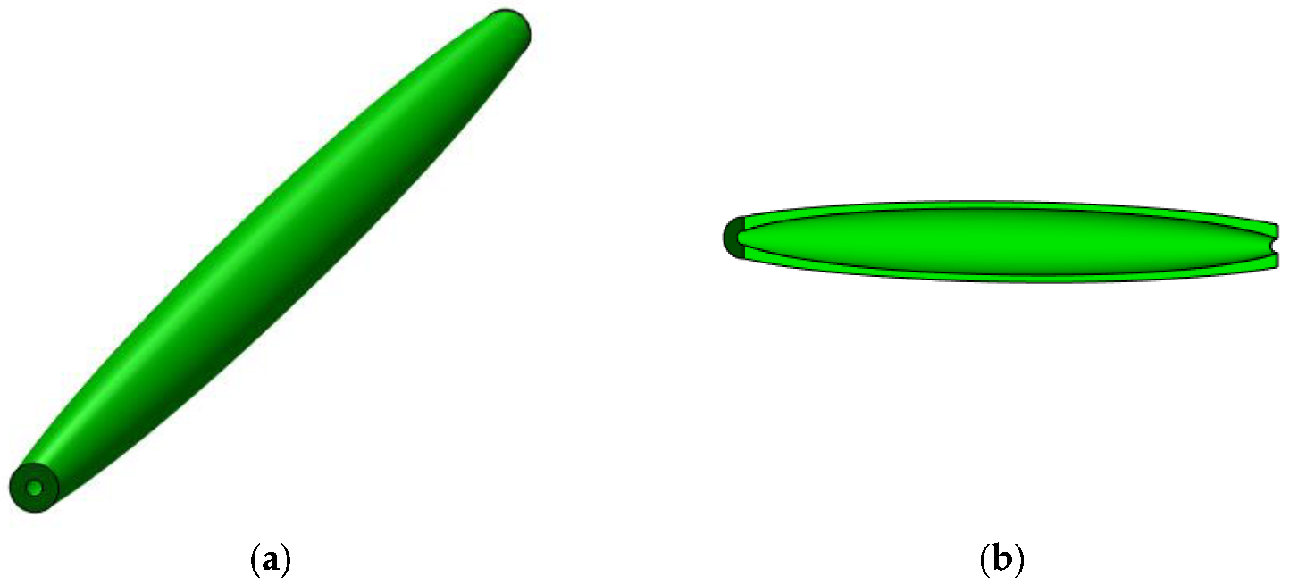
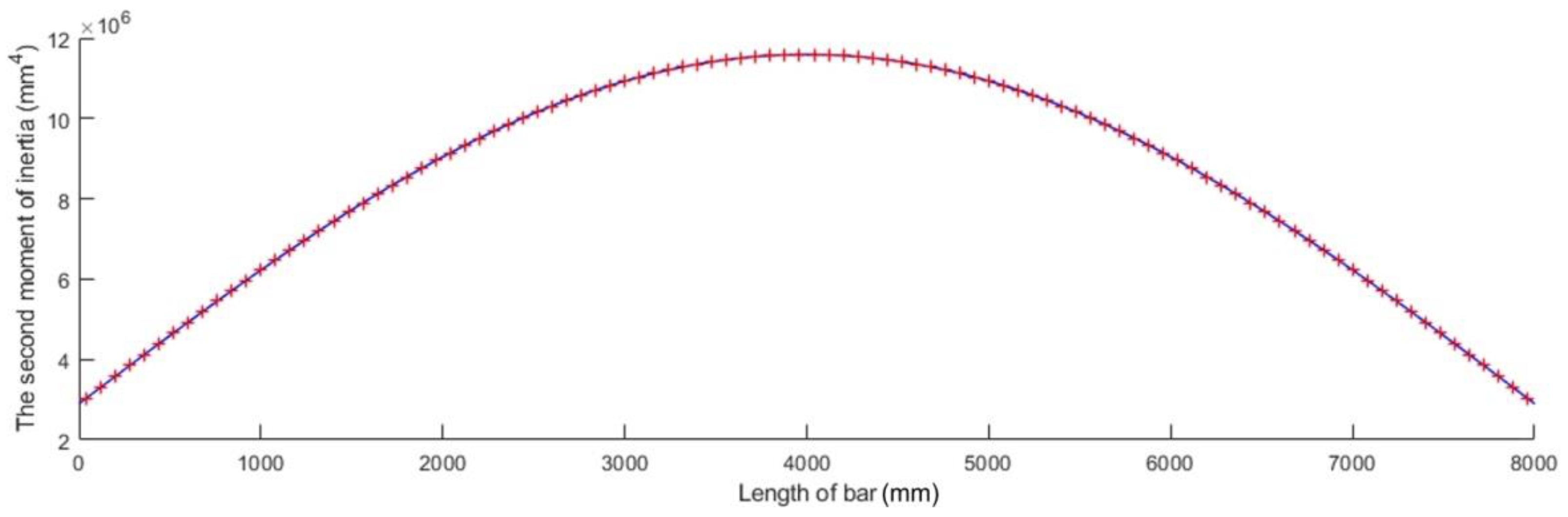
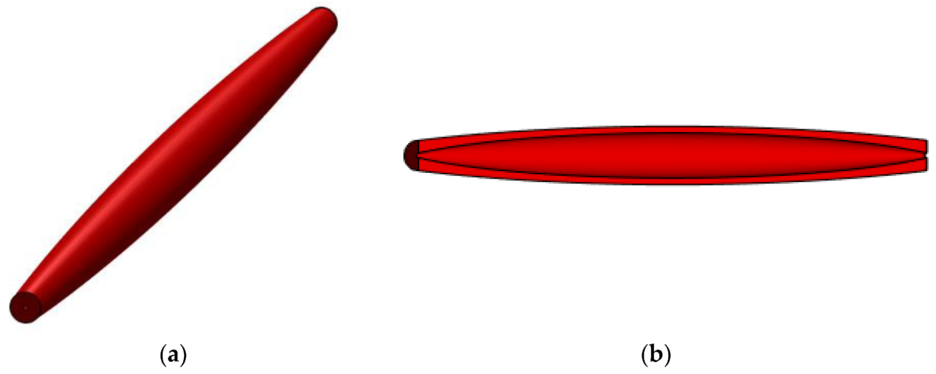
In
Table 2, two extreme cases were considered for bars whose the second moments of inertia were constant along the bar length
: (i) a bar having a second moment of inertia equal to
(code CONST_1I); and (ii) a bar having a second moment of inertia equal to
(code CONST_1I). For both cases, the length
of the bar was that given in
Table 1, and it was assumed that the bar had an annular cross-section. The value
for the second moment of inertia corresponded to an annular cross-section having an inner diameter
and an outer diameter
, which are also given in
Table 1. For the second bar, for which the second moment of inertia was equal to
, the inner diameter
and outer diameter
were computed by considering the area
of the annular cross-section in order for the normal stress in compression to be equal to the normal stress
at the proportionality limit (which was approximately equal to the normal stress at yielding
).
The results obtained using the numerical model with 32 finite elements were comparatively analyzed for all the types of columns shown in
Table 2.


