
Predicting Dynamic Properties of Asphalt Mastic Considering Asphalt–Filler Interaction Based on 2S2P1D Model

Abstract
:1. Introduction
2. Materials and Tests
2.1. Materials
2.2. Tests
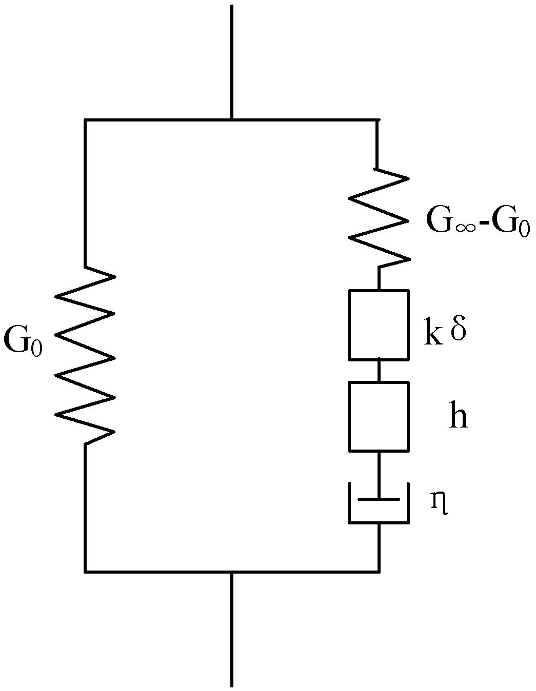
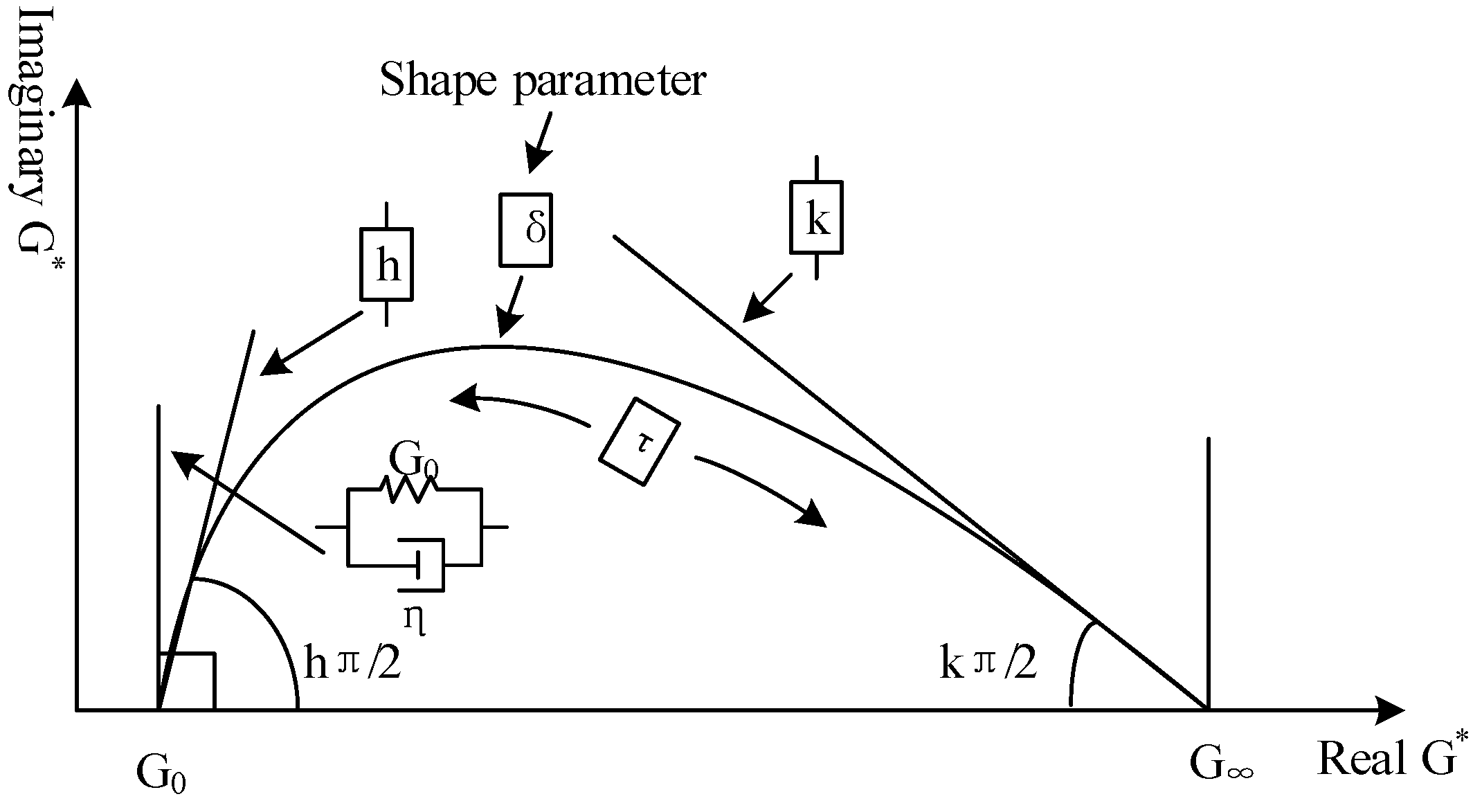
3. 2S2P1D Model
4. Result and Discussion
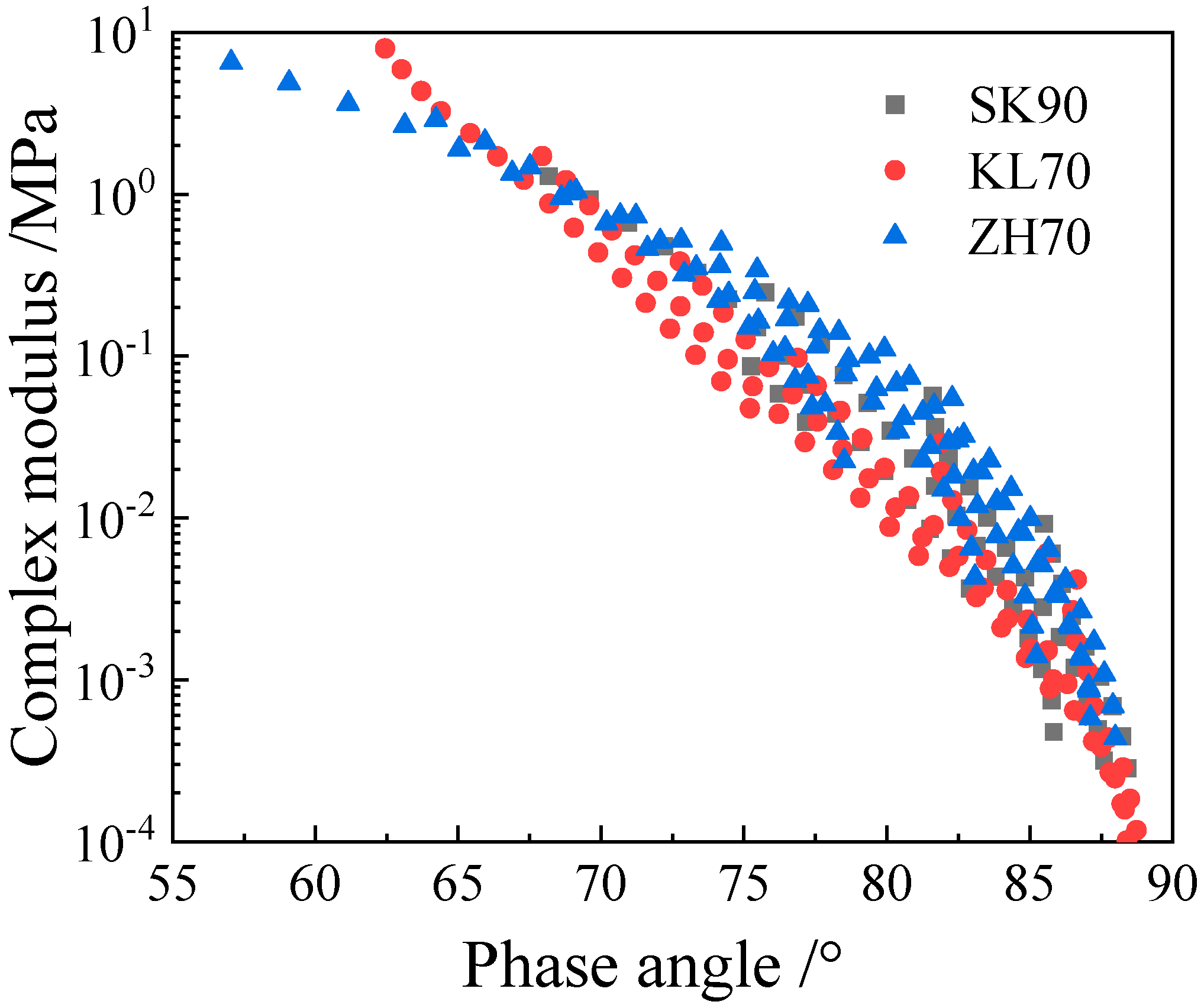
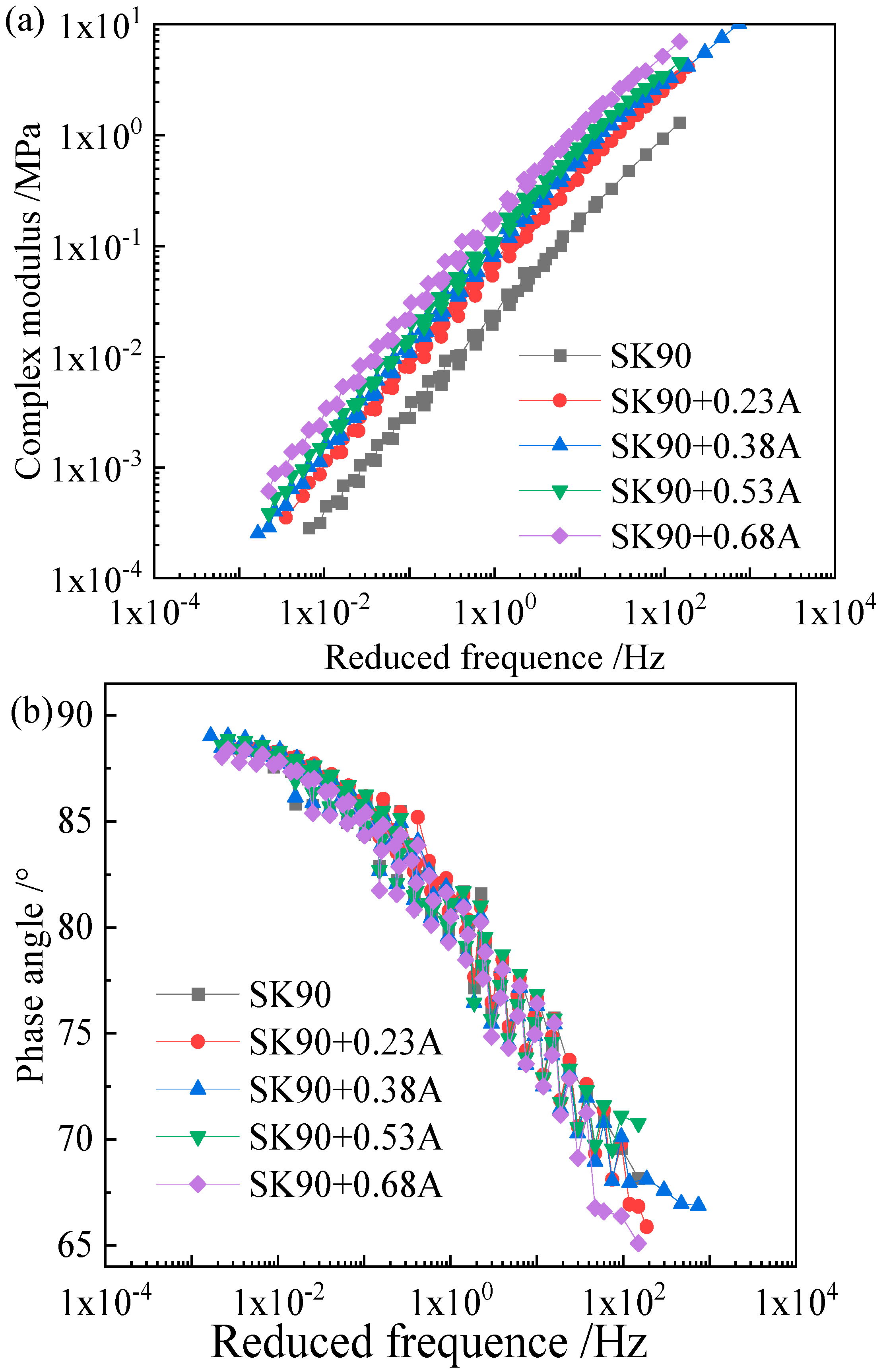
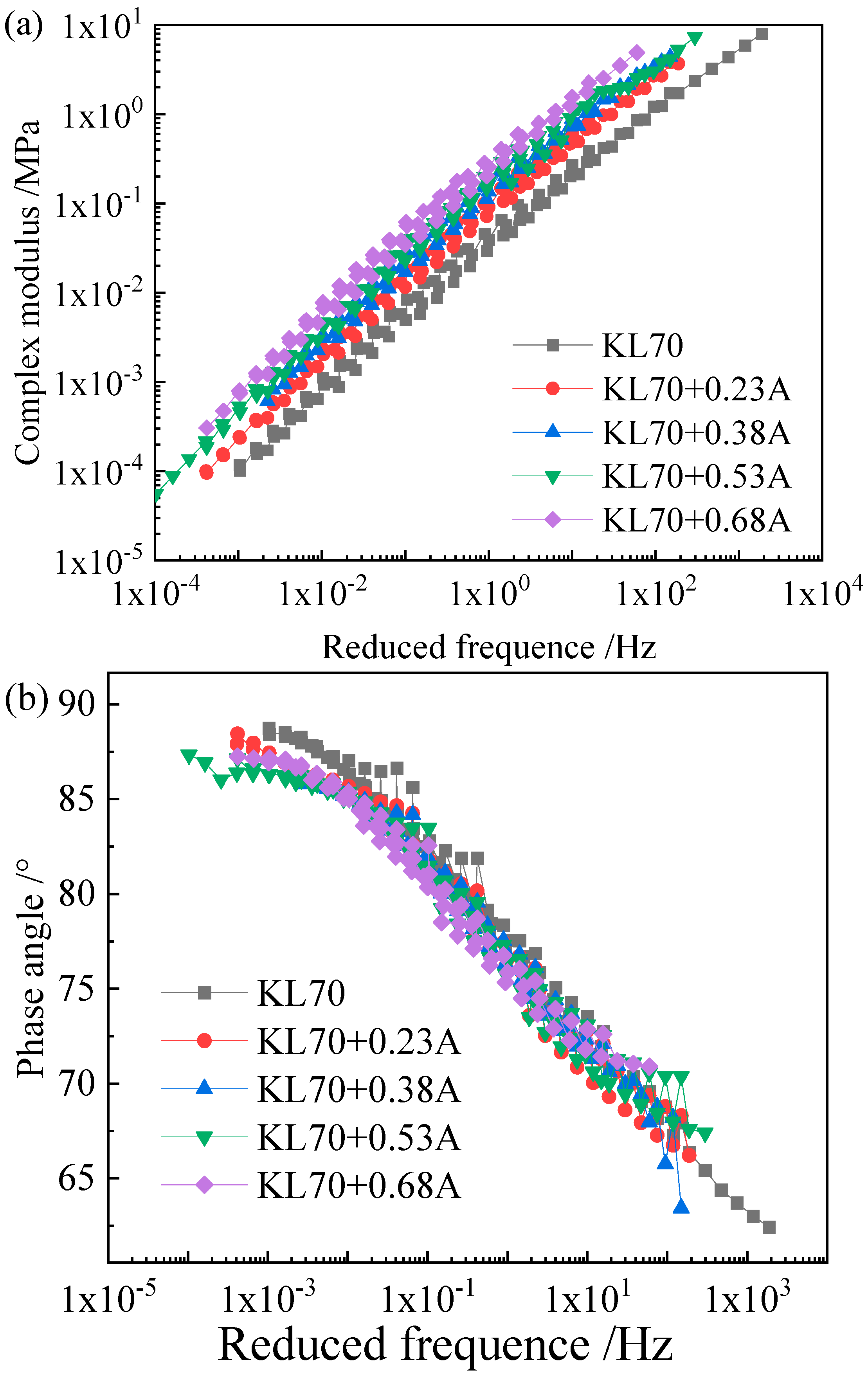
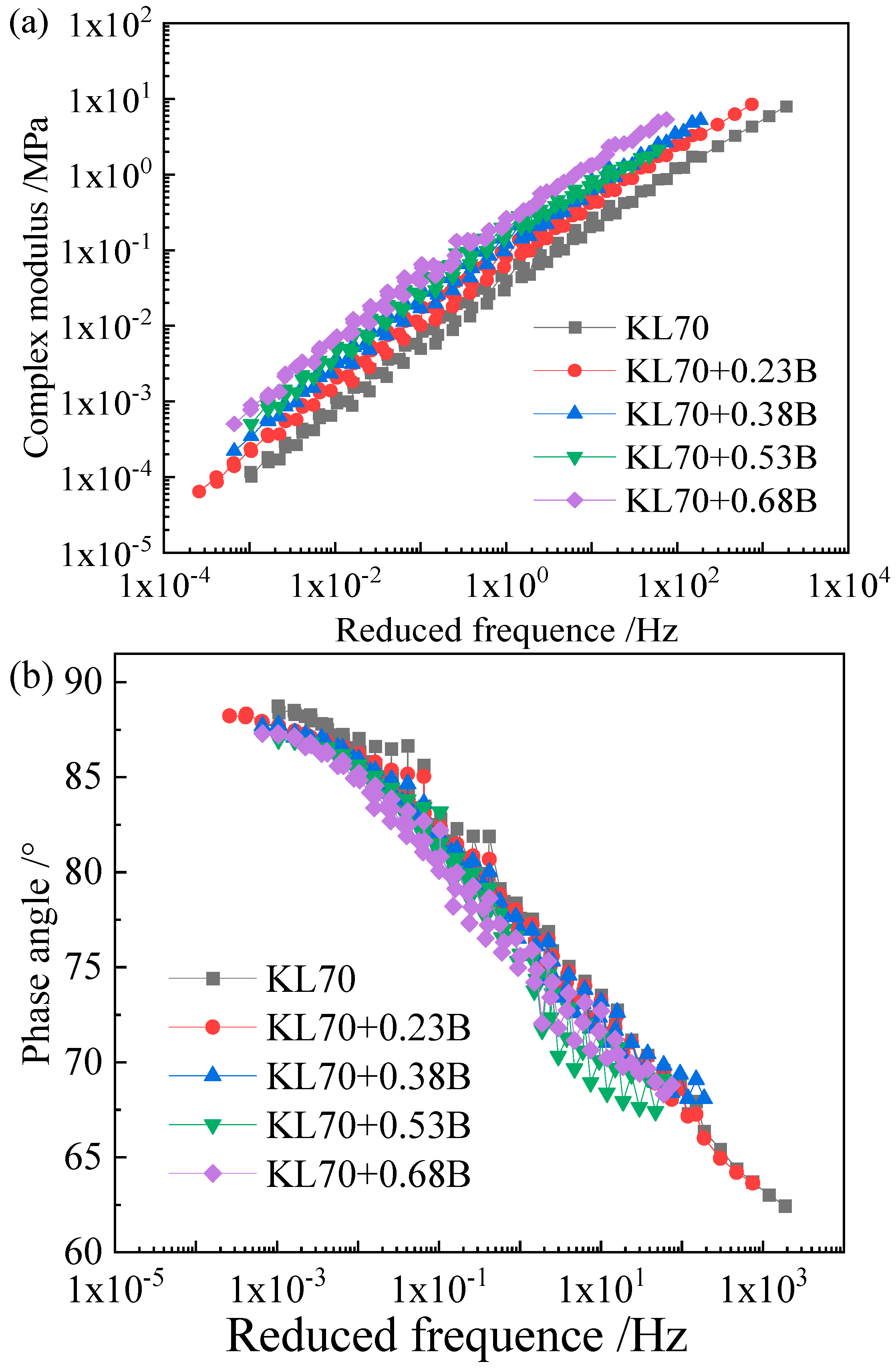
4.1. Test Result
4.2. The Interaction between Asphalt and Filler
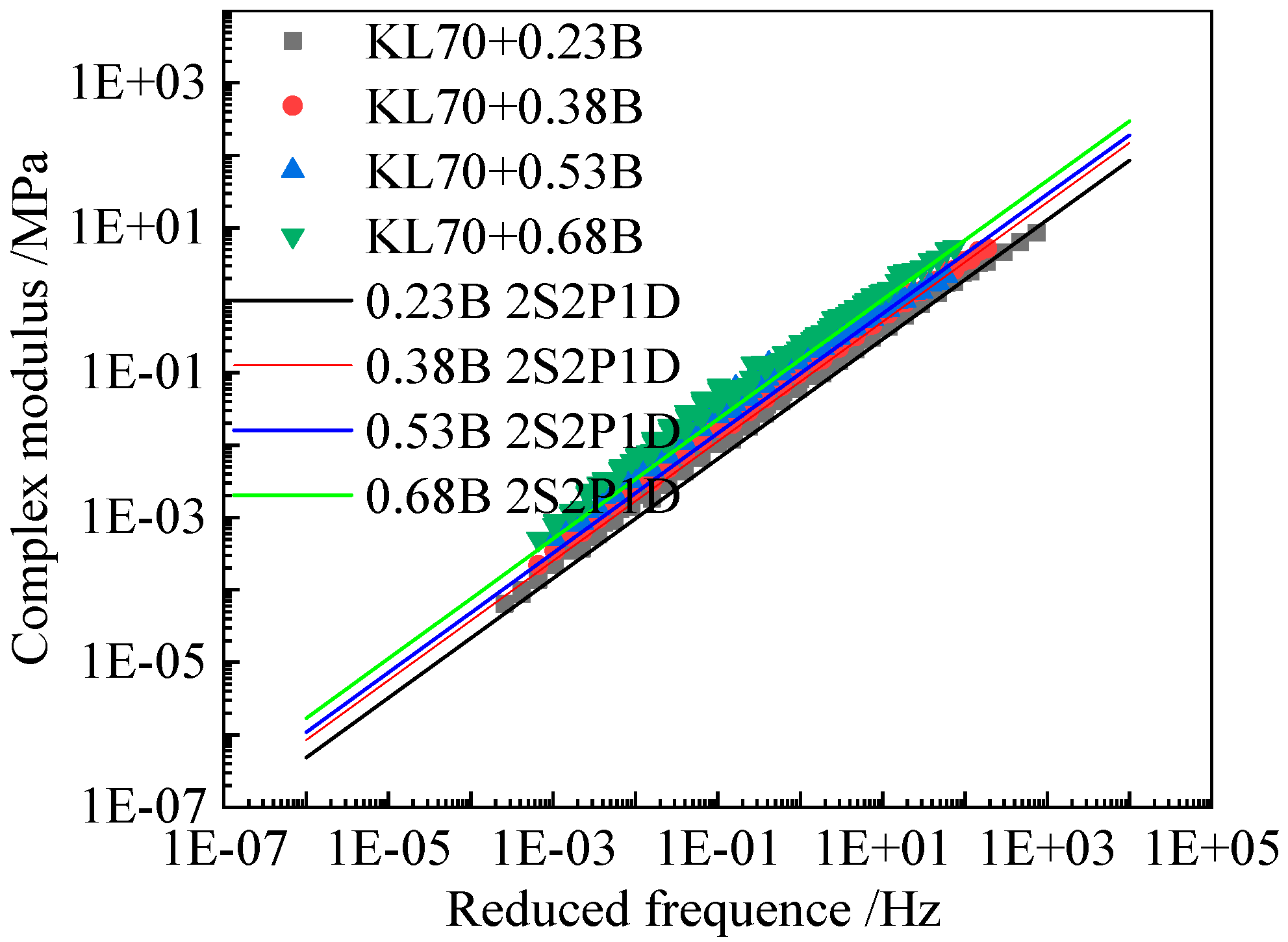
4.3. Calibration of the 2S2P1D Model
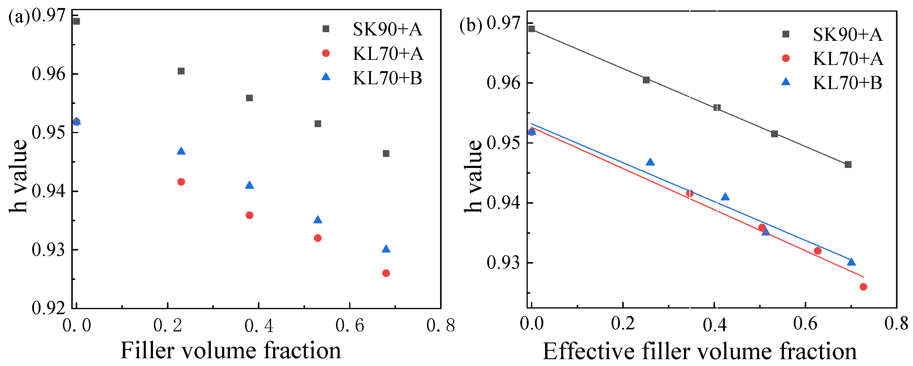
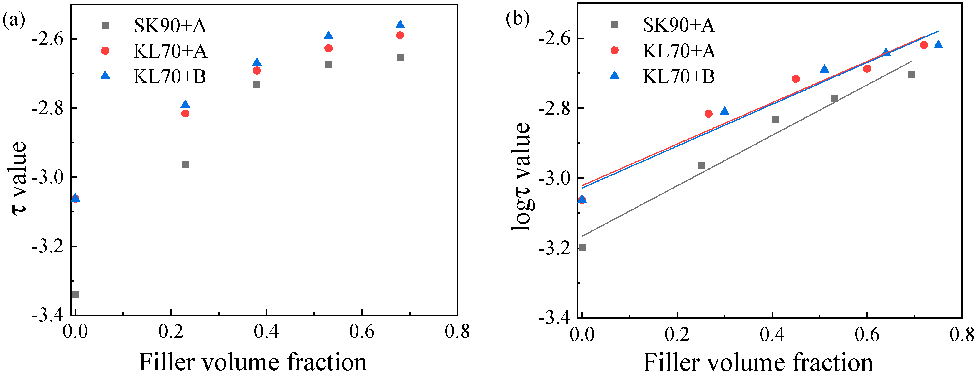
4.3.1. Determination of and
4.3.2. Relationship between the 2S2P1D Model Parameters of Asphalt and Corresponding Mastics
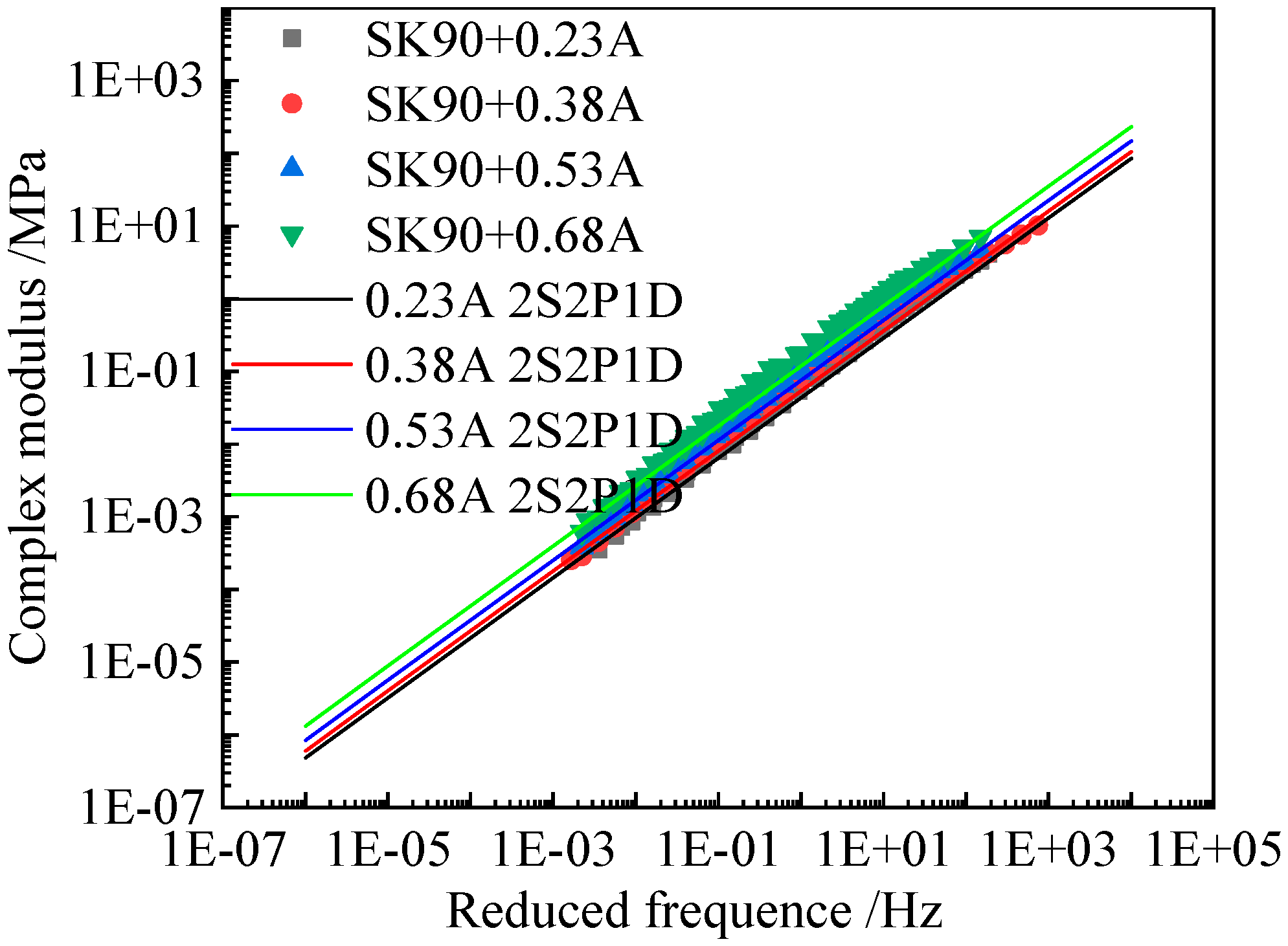
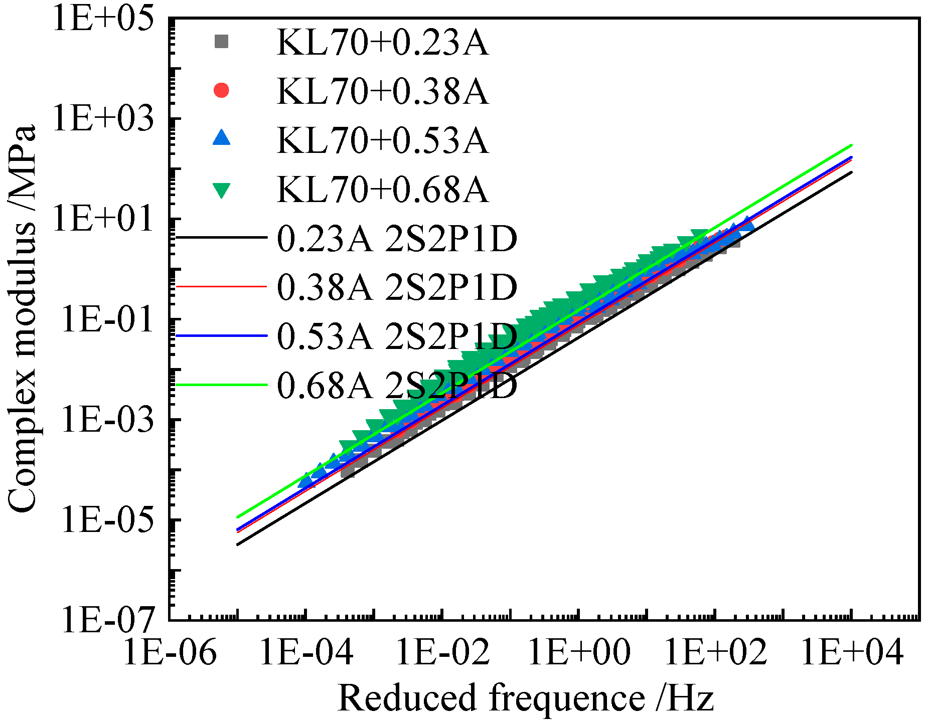
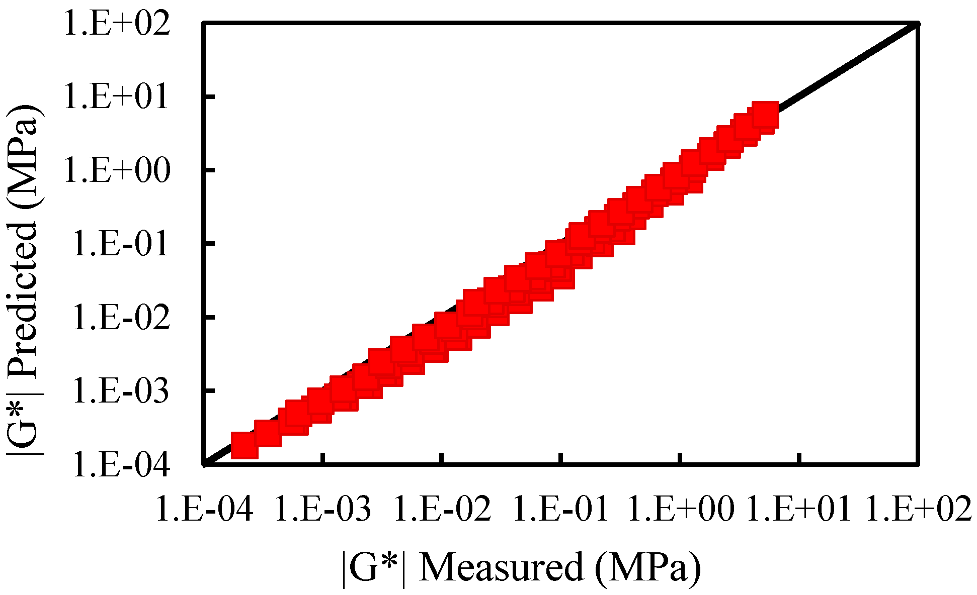
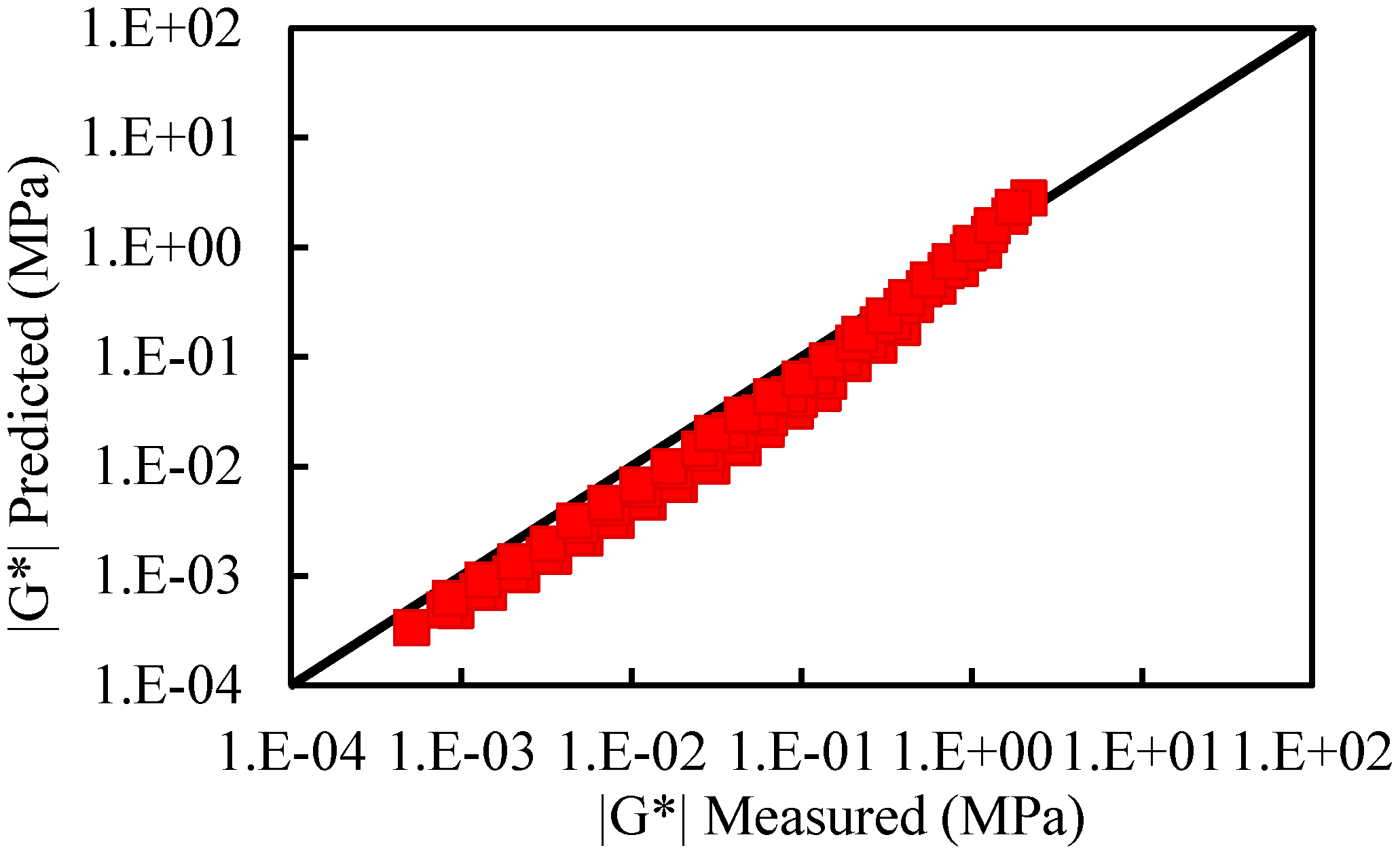
4.4. Validation
5. Conclusions
Author Contributions
Funding
Institutional Review Board Statement
Informed Consent Statement
Data Availability Statement
Acknowledgments
Conflicts of Interest
References
- Underwood, B.S.; Kim, Y.R. Microstructural investigation of asphalt concrete for performing multiscale experimental studies. Int. J. Pavement Eng. 2013, 14, 498–516. [Google Scholar] [CrossRef]
- Traxler, R.N.; Miller, J.S. Mineral powders, their physical properties and stabilizing effects. Assoc. Asph. Paving Technol 1936, 7, 112–123. [Google Scholar] [CrossRef]
- Antoni, S.; Piotr, M. Verification of bituminous mixtures rheological parameters through rutting test. Road Mater. Pavement Des. 2003, 4, 423–438. [Google Scholar]
- Riccardi, C.; Falchetto, A.C.; Michael, M.L. Rheological modeling of asphalt binder and asphalt mortar containing recycled asphalt material. Mater. Struct. 2015, 49, 85–92. [Google Scholar] [CrossRef]
- Yan, K.-Z.; Xu, H.-B.; Zhang, H.-L. Effect of mineral filler on properties of warm asphalt mastic containing Sasobit. Constr. Build. Mater. 2013, 48, 622–627. [Google Scholar] [CrossRef]
- Buttlar, W.G.; Bozkurt, D.; Al-Khateeb, G.G. Understanding Asphalt Mastic Behavior through micromechanics. Transp. Res. Rec. 1999, 1681, 157–169. [Google Scholar] [CrossRef]
- Fakhari Tehrani, F.; Absi, J.; Allou, F.; Petit, C. Investigation into the impact of the use of 2D/3D digital models on the numerical calculation of the bituminous composites’ complex modulus. Comput. Mater. Sci. 2013, 79, 377–389. [Google Scholar] [CrossRef]
- Yin, H.M.; Buttlar, W.G.; Paulino, G.H.; Benedetto, H.D. Assessment of Existing Micro-mechanical Models for Asphalt Mastics Considering Viscoelastic Effects. Road Mater. Pavement Des. 2011, 9, 31–57. [Google Scholar] [CrossRef]
- Yong-Rak Kim, D.N.L. Linear viscoelastic analysis of asphalt mastics. J. Mater. Civ. Eng. 2014, 16, 11. [Google Scholar] [CrossRef]
- Hajikarimi, P.; Fakhari Tehrani, F.; Moghadas Nejad, F.; Absi, J.; Khodaii, A.; Rahi, M.; Petit, C. Mechanical Behavior of Polymer-Modified Bituminous Mastics. II: Numerical Approach. J. Mater. Civ. Eng. 2019, 31, 04018338. [Google Scholar] [CrossRef]
- Pei, J.; Fan, Z.; Wang, P.; Zhang, J.; Xue, B.; Li, R. Micromechanics prediction of effective modulus for asphalt mastic considering inter-particle interaction. Constr. Build. Mater. 2015, 101, 209–216. [Google Scholar] [CrossRef]
- Guo, M.; Bhasin, A.; Tan, Y. Effect of mineral fillers adsorption on rheological and chemical properties of asphalt binder. Constr. Build. Mater. 2017, 141, 152–159. [Google Scholar] [CrossRef]
- Antunes, V.; Freire, A.C.; Quaresma, L.; Micaelo, R. Effect of the chemical composition of fillers in the filler–bitumen interaction. Constr. Build. Mater. 2016, 104, 85–91. [Google Scholar] [CrossRef]
- Tan, Y.; Guo, M. Interfacial thickness and interaction between asphalt and mineral fillers. Mater. Struct. 2013, 47, 605–614. [Google Scholar] [CrossRef]
- Tan, Y.; Guo, M. Micro- and Nano-Characteration of Interaction between Asphalt and Filler. J. Test. Eval. 2014, 42, 1089–1097. [Google Scholar] [CrossRef]
- Underwood, B.S.; Kim, Y.R. A four phase micro-mechanical model for asphalt mastic modulus. Mech. Mater. 2014, 75, 13–33. [Google Scholar] [CrossRef]
- Olard, F.; Di Benedetto, H. General “2S2P1D” Model and Relation Between the Linear Viscoelastic Behaviours of Bituminous Binders and Mixes. Road Mater. Pavement Des. 2011, 4, 185–224. [Google Scholar] [CrossRef]
- Riccardi, C.; Cannone Falchetto, A.; Losa, M.; Leandri, P. Estimation of the SHStS transformation parameter based on volumetric composition. Constr. Build. Mater. 2017, 157, 244–252. [Google Scholar] [CrossRef]
- Riccardi, C.; Cannone Falchetto, A.; Losa, M.; Wistuba, M.P. Development of simple relationship between asphalt binder and mastic based on rheological tests. Road Mater. Pavement Des. 2016, 19, 18–35. [Google Scholar] [CrossRef]
- Yusoff, N.I.M.; Jakarni, F.M.; Nguyen, V.H.; Hainin, M.R.; Airey, G.D. Modelling the rheological properties of bituminous binders using mathematical equations. Constr. Build. Mater. 2013, 40, 174–188. [Google Scholar] [CrossRef]
- Yusoff, N.I.M.; Mounier, D.; Marc-Stéphane, G.; Rosli Hainin, M.; Airey, G.D.; Di Benedetto, H. Modelling the rheological properties of bituminous binders using the 2S2P1D Model. Constr. Build. Mater. 2013, 38, 395–406. [Google Scholar] [CrossRef]
- Di Benedetto, H.; Olard, F.; Sauzéat, C.; Delaporte, B. Linear viscoelastic behaviour of bituminous materials: From binders to mixes. Road Mater. Pavement Des. 2011, 5, 163–202. [Google Scholar] [CrossRef]
- Benveniste, Y. A New Approach to the Application of Mori-Tanaka’s Theory in Composite Materials. Mech. Mater. 1987, 6, 147–157. [Google Scholar] [CrossRef]


| Asphalt | Penetration 25 °C/0.1 mm | Soft Point/°C | Ductility/cm | PG/°C |
|---|---|---|---|---|
| SK90 | 83.0 | 45.5 | 85 (10 °C) | 52–28 |
| KL70 | 65.5 | 48.0 | 63 (10 °C) | 58–22 |
| ZH70 | 63.0 | 47.5 | 50 (10 °C) | 58–22 |
| Asphalt Mastic | 0.32 | 0.38 | 0.53 | 0.68 |
|---|---|---|---|---|
| SK90 + filler (A) | 1.76 | 1.38 | 1.12 | 1.06 |
| KL70 + filler (A) | 1.44 | 1.28 | 1.08 | 1.02 |
| KL70 + filler (B) | 1.29 | 1.25 | 1.07 | 1.04 |
| Asphalt | Mastic | δ | k | h | β | log(τ0) | G0 (MPa) | G0 (MPa) |
|---|---|---|---|---|---|---|---|---|
| SK90 | 0 | 10 | 0.9649 | 0.9649 | 1.83 × 10⁸ | −3.3392 | 0 | 1000 |
| 0.23A | 10 | 0.9615 | 0.9615 | 1.83 × 10⁸ | −2.9635 | 0.61 × 10⁻⁶ | 1290 | |
| 0.38A | 10 | 0.9559 | 0.9559 | 1.83 × 10⁸ | −2.6916 | 1.39 × 10⁻⁶ | 1540 | |
| 0.53A | 10 | 0.9515 | 0.9515 | 1.83 × 10⁸ | −2.6736 | 2.50 × 10⁻⁶ | 1660 | |
| 0.68A | 10 | 0.9464 | 0.9464 | 1.83 × 10⁸ | −2.6547 | 5.69 × 10⁻⁶ | 1840 | |
| KL70 | 0 | 10 | 0.9518 | 0.9518 | 1.83 × 10⁸ | −3.0624 | 0 | 1000 |
| 0.23A | 10 | 0.9416 | 0.9416 | 1.83 × 10⁸ | −2.8158 | 2.59 × 10⁻⁶ | 1420 | |
| 0.38A | 10 | 0.9359 | 0.9359 | 1.83 × 10⁸ | −2.6916 | 4.19 × 10⁻⁶ | 1690 | |
| 0.53A | 10 | 0.9340 | 0.9340 | 1.83 × 10⁸ | −2.627 | 9.40 × 10⁻⁶ | 1780 | |
| 0.68A | 10 | 0.9311 | 0.9311 | 1.83 × 10⁸ | −2.4894 | 14.70 × 10⁻⁶ | 2000 | |
| KL70 | 0 | 10 | 0.9518 | 0.9519 | 1.83 × 10⁸ | −3.0624 | 0 | 1000 |
| 0.23B | 10 | 0.9467 | 0.9467 | 1.83 × 10⁸ | −2.8310 | 2.54 × 10⁻⁶ | 1490 | |
| 0.38B | 10 | 0.9409 | 0.9409 | 1.83 × 10⁸ | −2.6701 | 5.04 × 10⁻⁶ | 1680 | |
| 0.53B | 10 | 0.9350 | 0.9350 | 1.83 × 10⁸ | −2.5925 | 11.44 × 10⁻⁶ | 1800 | |
| 0.68B | 10 | 0.9339 | 0.9339 | 1.83 × 10⁸ | −2.4603 | 15.30 × 10⁻⁶ | 1920 |
| Function | y = y0 + bx | ||
|---|---|---|---|
| Asphalt | SK90 + A | KL70 + A | KL70 + B |
| y0 | 0.9689 ± 0.0010 | 0.9523 ± 0.0012 | 0.9532 ± 0.0016 |
| b | −0.0325 ± 3.7584 × 10⁻⁴ | −0.0331 ± 0.0023 | −0.0324 ± 0.0035 |
| Sum squared residual | 1.2003 × 10⁻⁷ | 5.3941 × 10⁻⁶ | 1.0441 × 10⁻⁵ |
| R2 | 0.9996 | 0.986 | 0.965 |
| 0.9994 | 0.981 | 0.954 | |
| Function | y = y0 + bx | ||
|---|---|---|---|
| Asphalt | SK90 + A | KL70 + A | KL70 + B |
| y0 | −3.16626 ± 0.03367 | −3.02115 ± 0.03945 | −3.02811 ± 0.03676 |
| b | 0.62132 ± 0.07555 | 0.59193 ± 0.08219 | 0.59784 ± 0.07148 |
| Reduced Chi-Sqr | 0.00485 | 0.00654 | 0.00543 |
| R2 | 0.9681 | 0.9722 | 0.9792 |
| 0.9575 | 0.96532 | 0.9688 | |
Publisher’s Note: MDPI stays neutral with regard to jurisdictional claims in published maps and institutional affiliations. |
© 2022 by the authors. Licensee MDPI, Basel, Switzerland. This article is an open access article distributed under the terms and conditions of the Creative Commons Attribution (CC BY) license (https://creativecommons.org/licenses/by/4.0/).
Share and Cite
Ma, X.; Zhang, X.; Hou, J.; Song, S.; Chen, H.; Kuang, D. Predicting Dynamic Properties of Asphalt Mastic Considering Asphalt–Filler Interaction Based on 2S2P1D Model. Materials 2022, 15, 5688. https://doi.org/10.3390/ma15165688
Ma X, Zhang X, Hou J, Song S, Chen H, Kuang D. Predicting Dynamic Properties of Asphalt Mastic Considering Asphalt–Filler Interaction Based on 2S2P1D Model. Materials. 2022; 15(16):5688. https://doi.org/10.3390/ma15165688
Chicago/Turabian StyleMa, Xiaoyan, Xingyu Zhang, Junpeng Hou, Shanglin Song, Huaxin Chen, and Dongliang Kuang. 2022. "Predicting Dynamic Properties of Asphalt Mastic Considering Asphalt–Filler Interaction Based on 2S2P1D Model" Materials 15, no. 16: 5688. https://doi.org/10.3390/ma15165688