A Multiscale Topographical Analysis Based on Morphological Information: The HEVC Multiscale Decomposition

 , ,
, , 
Abstract
:
1. Introduction
2. Materials and Methods
2.1. Surface Processing
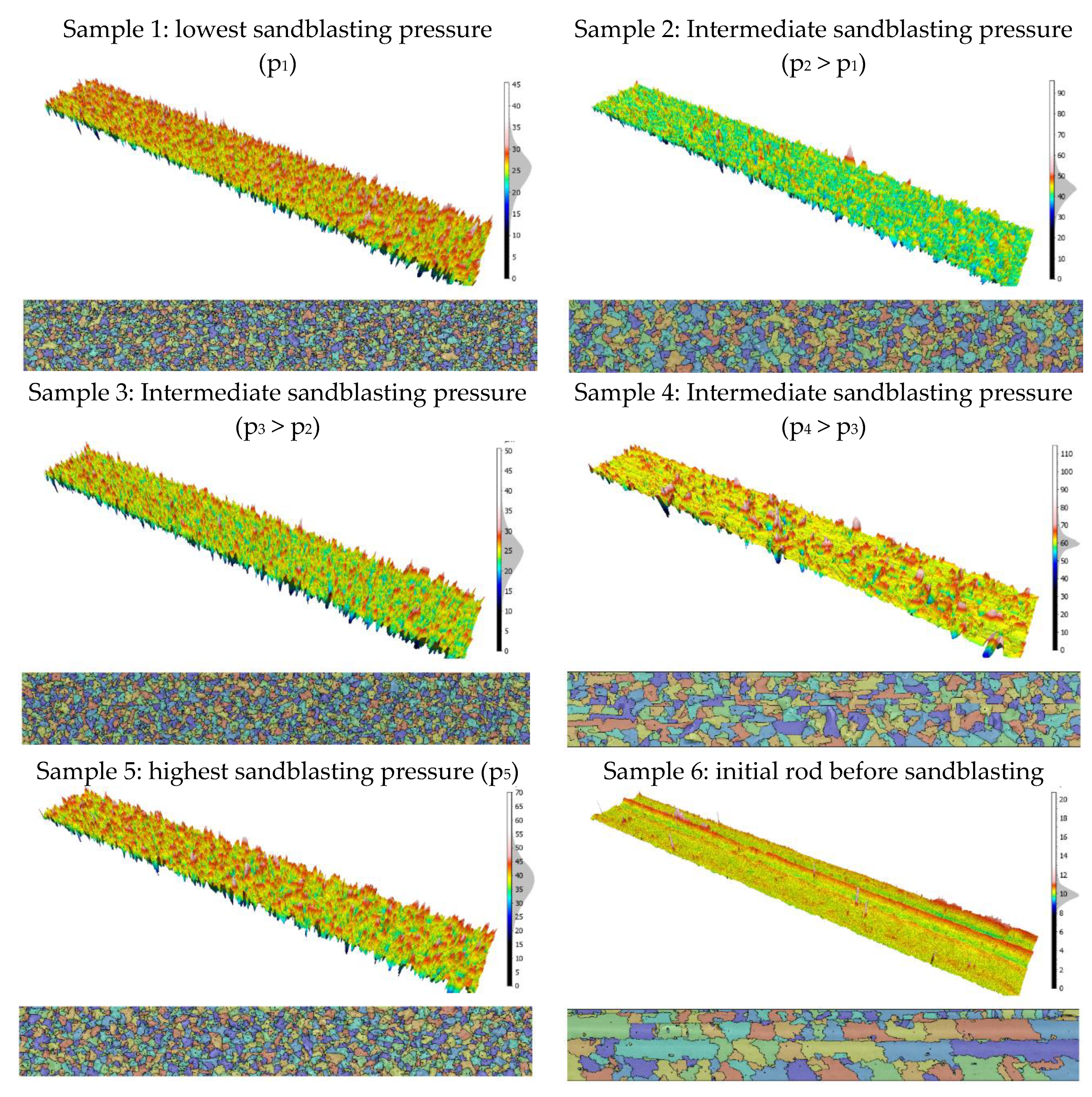
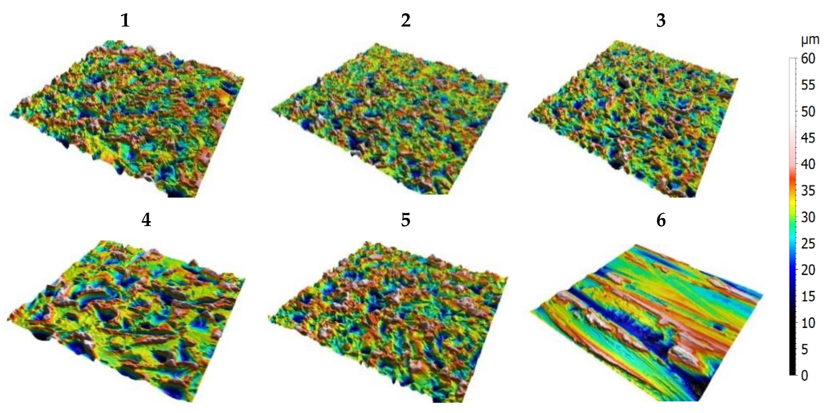
2.1.1. Surface Texturing
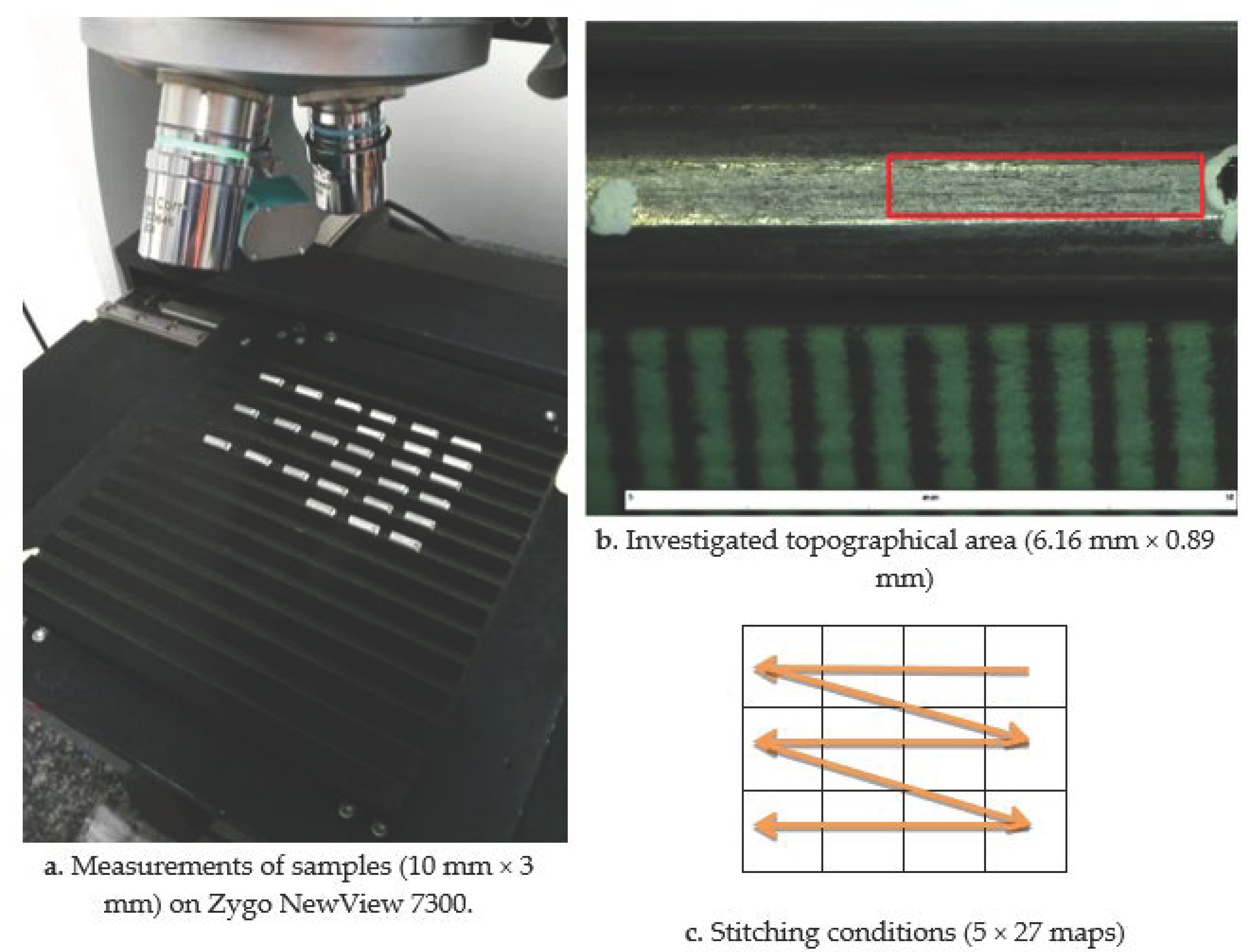
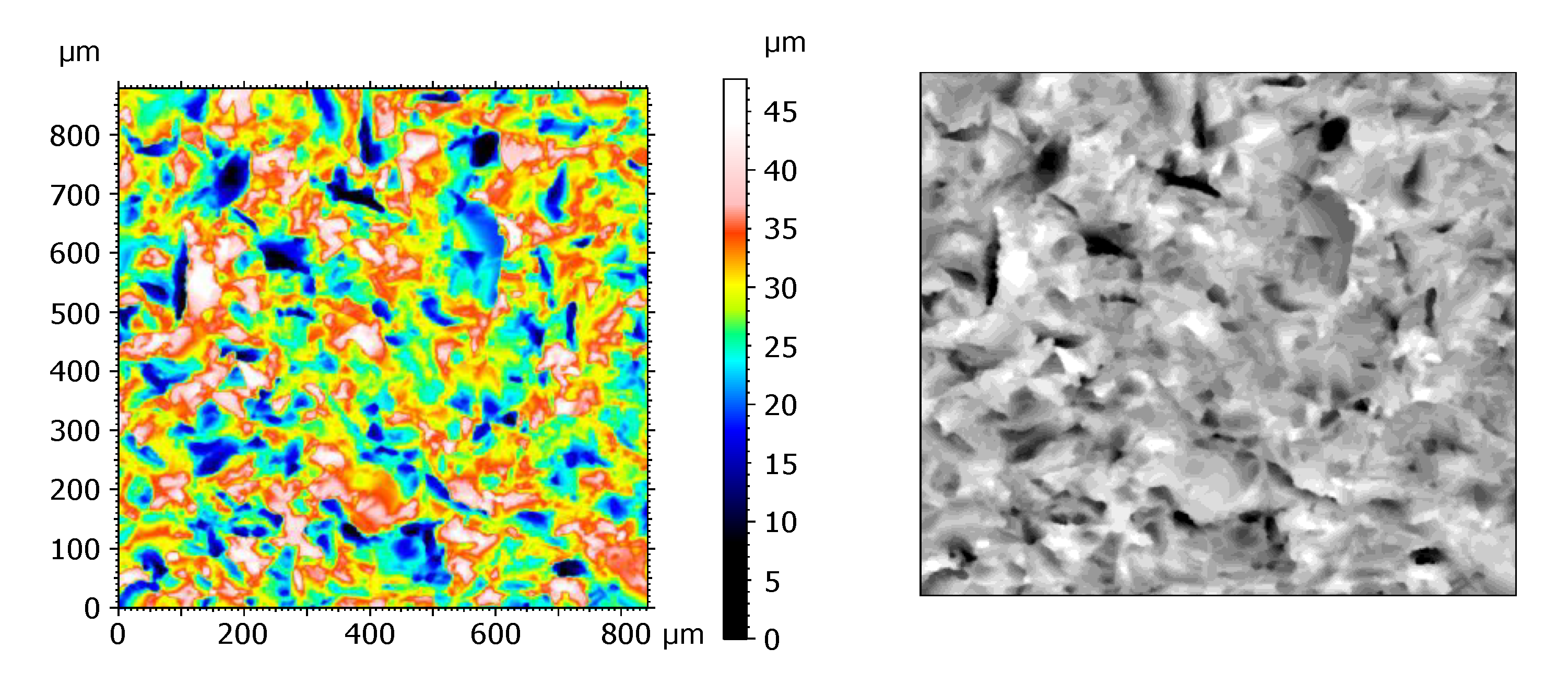
2.1.2. Topographical Measurements
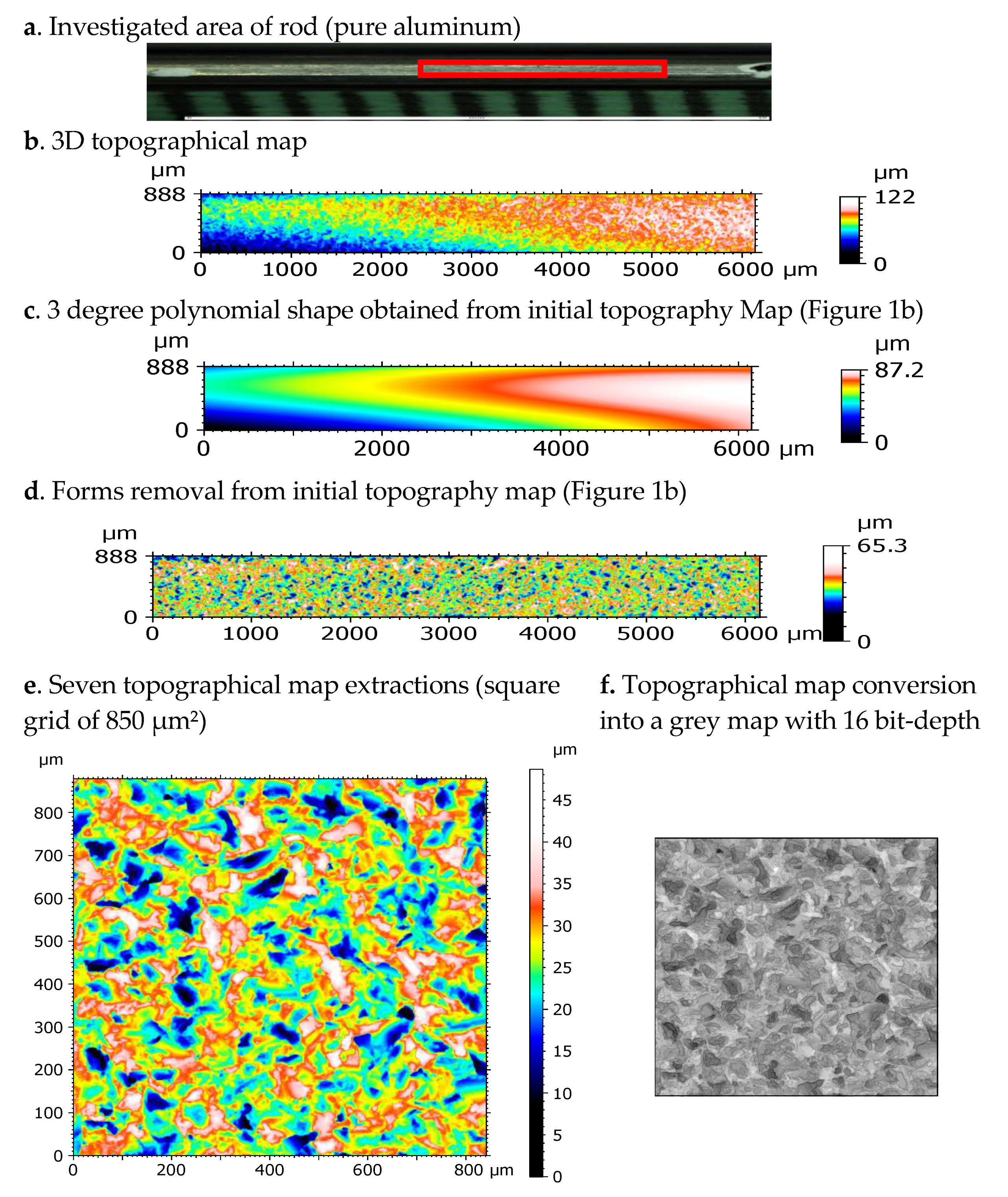
2.1.3. Surface Pretreatment
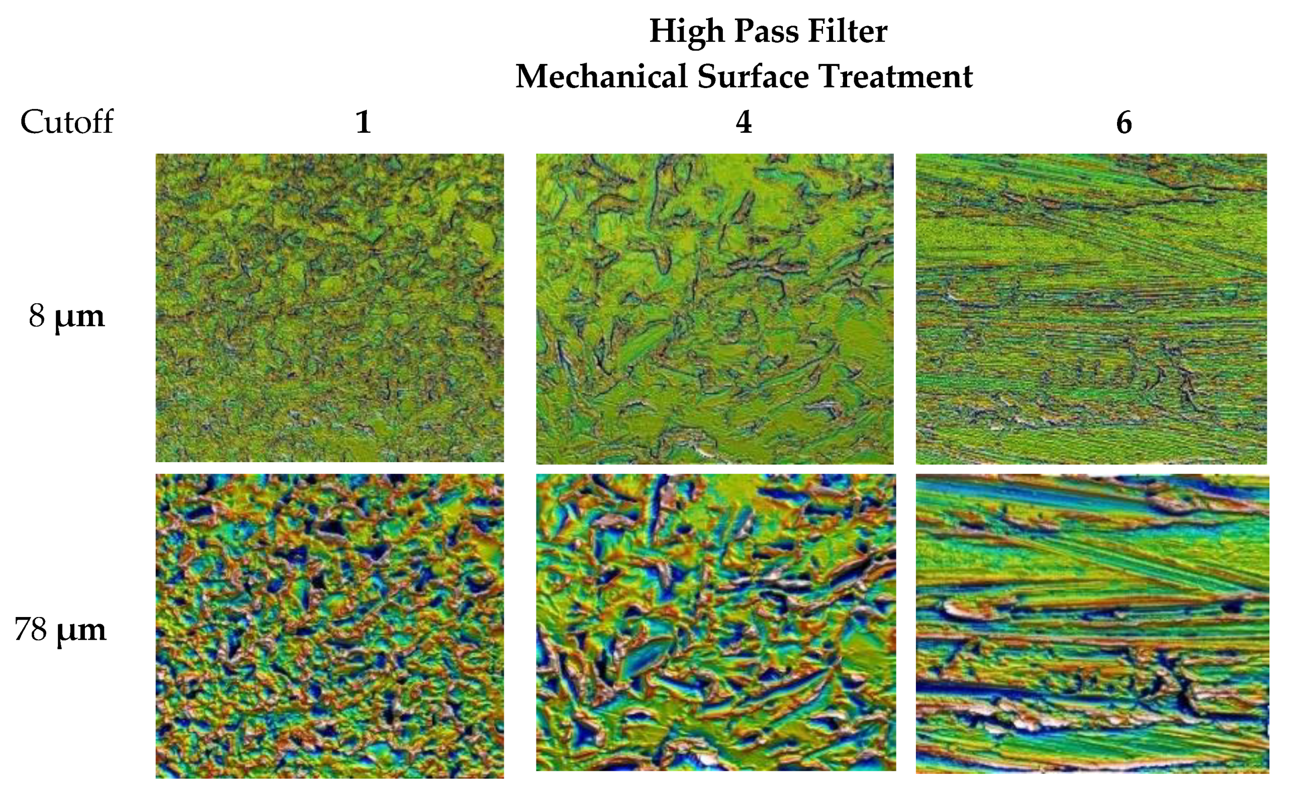
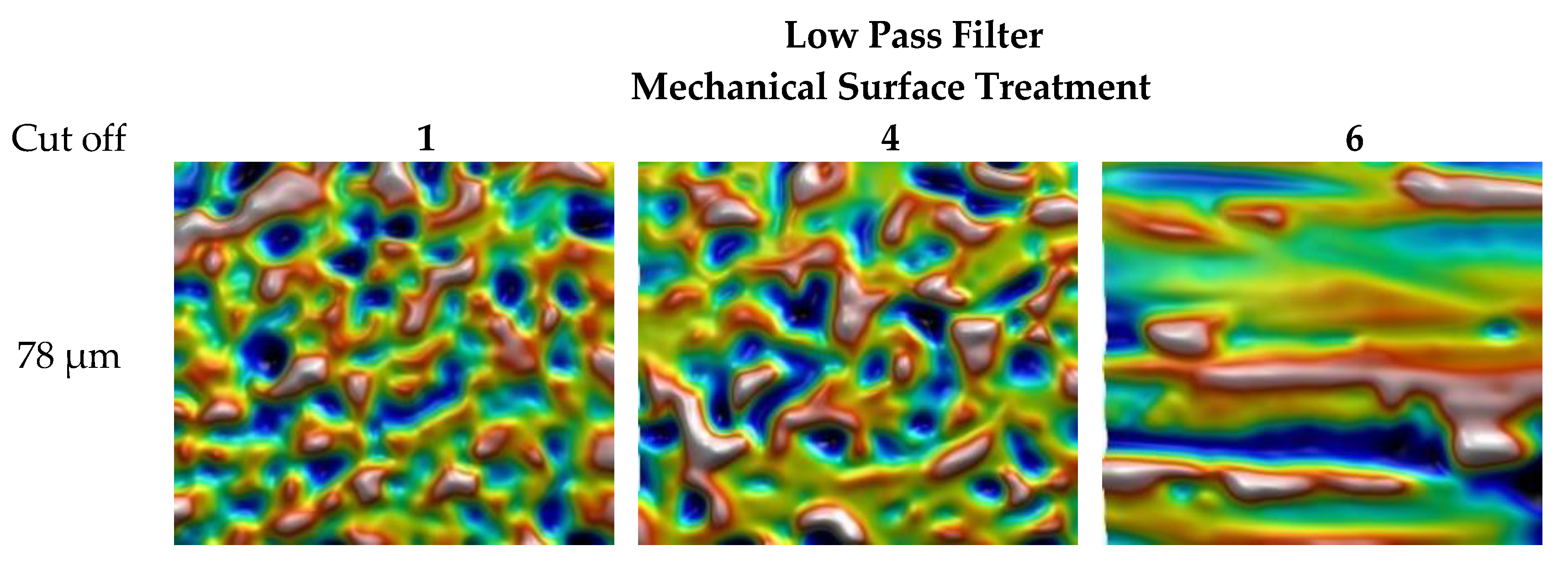
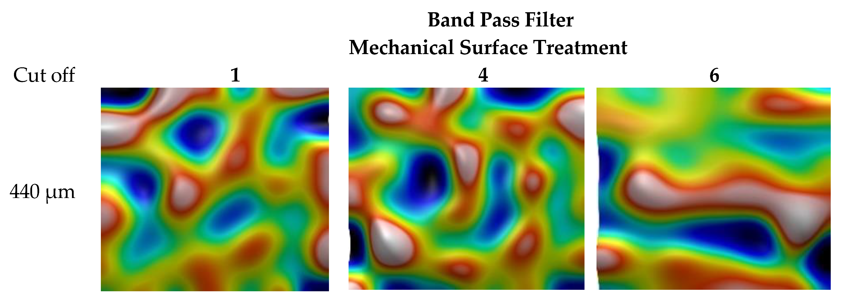
2.1.4. Multiscale Roughness Analysis
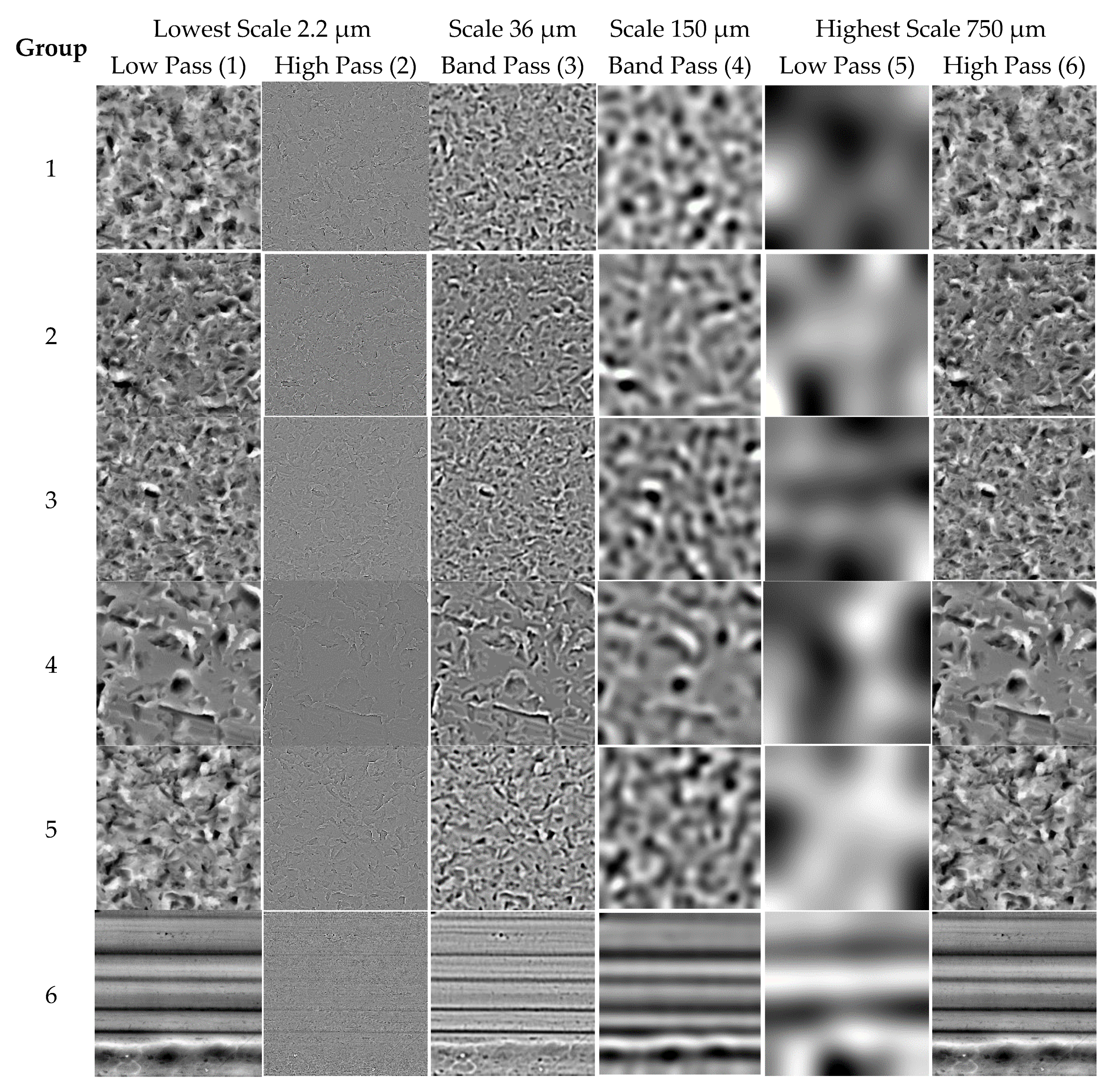
2.2. Topographical Materials Texture Image Data Set
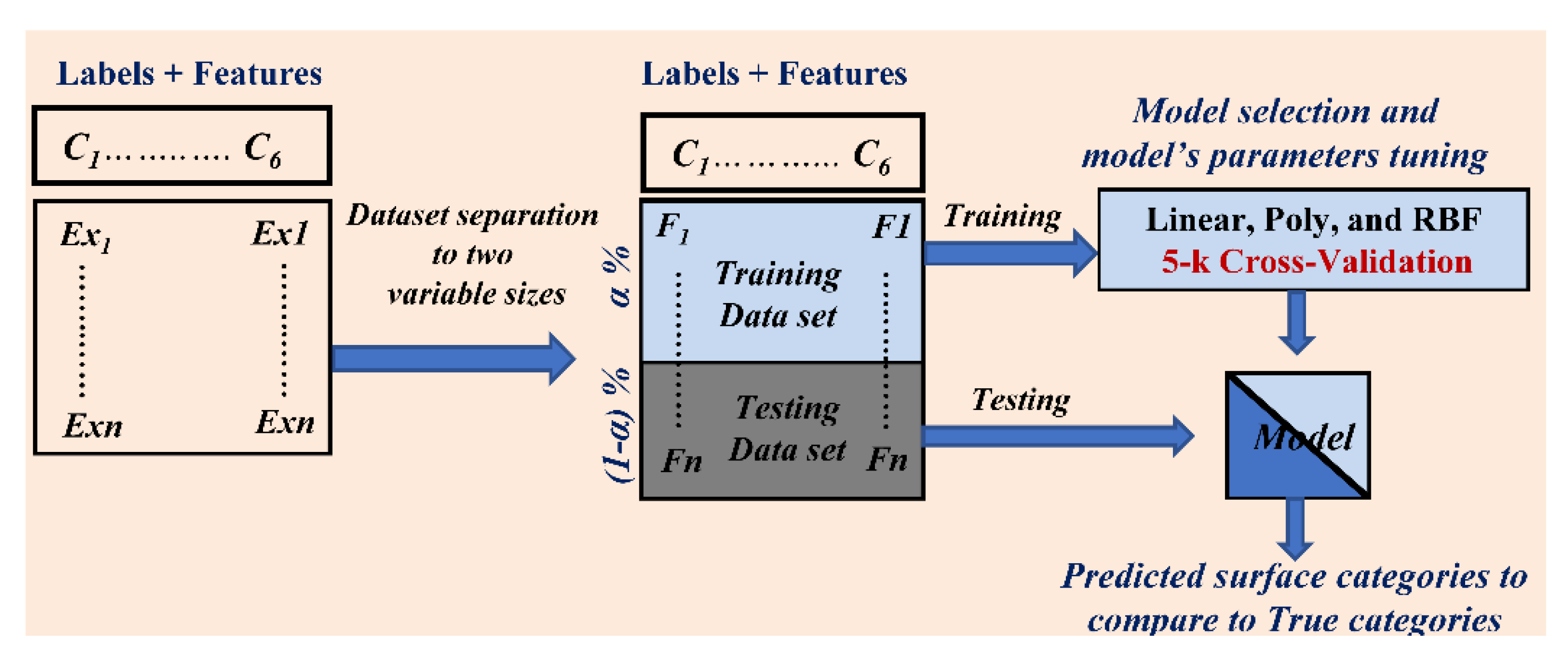
2.3. Topographical Analysis from the GPS ISO 25178 Standard Using SVM Decomposition
2.4. Information, Lossless Compression, and Topographical Caracterisation
3. Description of the Proposed Algorithm
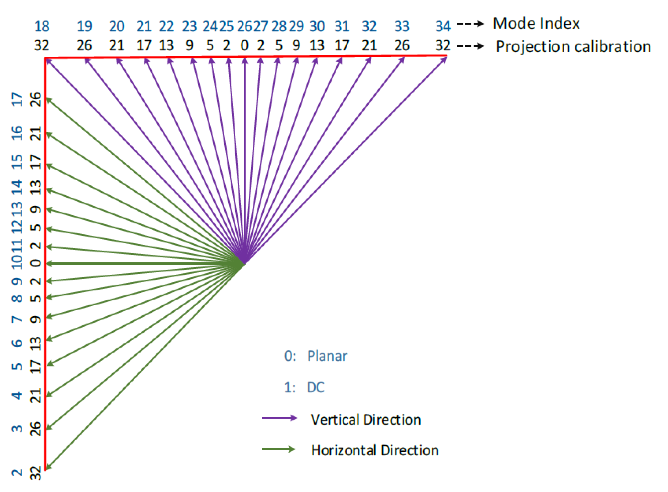
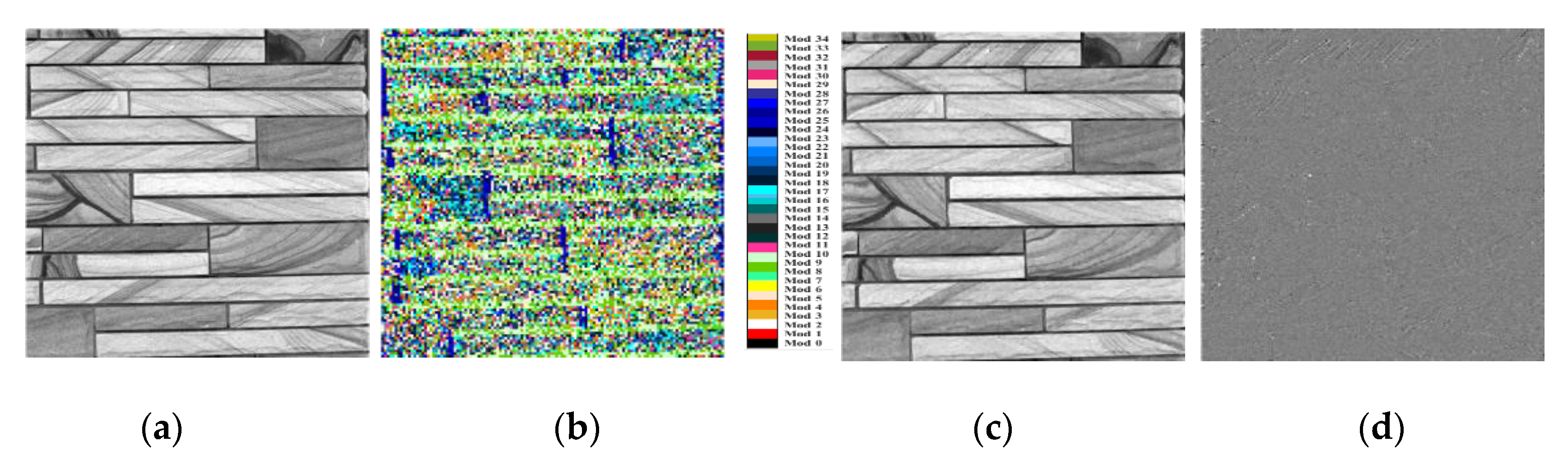
3.1. HEVC Intra-Prediction Coding
- HEVC Main 4:4:4 16 Still Picture (MSP) profile only considers intra-coding;
- Main-RExt (main_444_16_intra) and High Throughput 4:4:4 16 Intra apply both intra- and inter-coding.
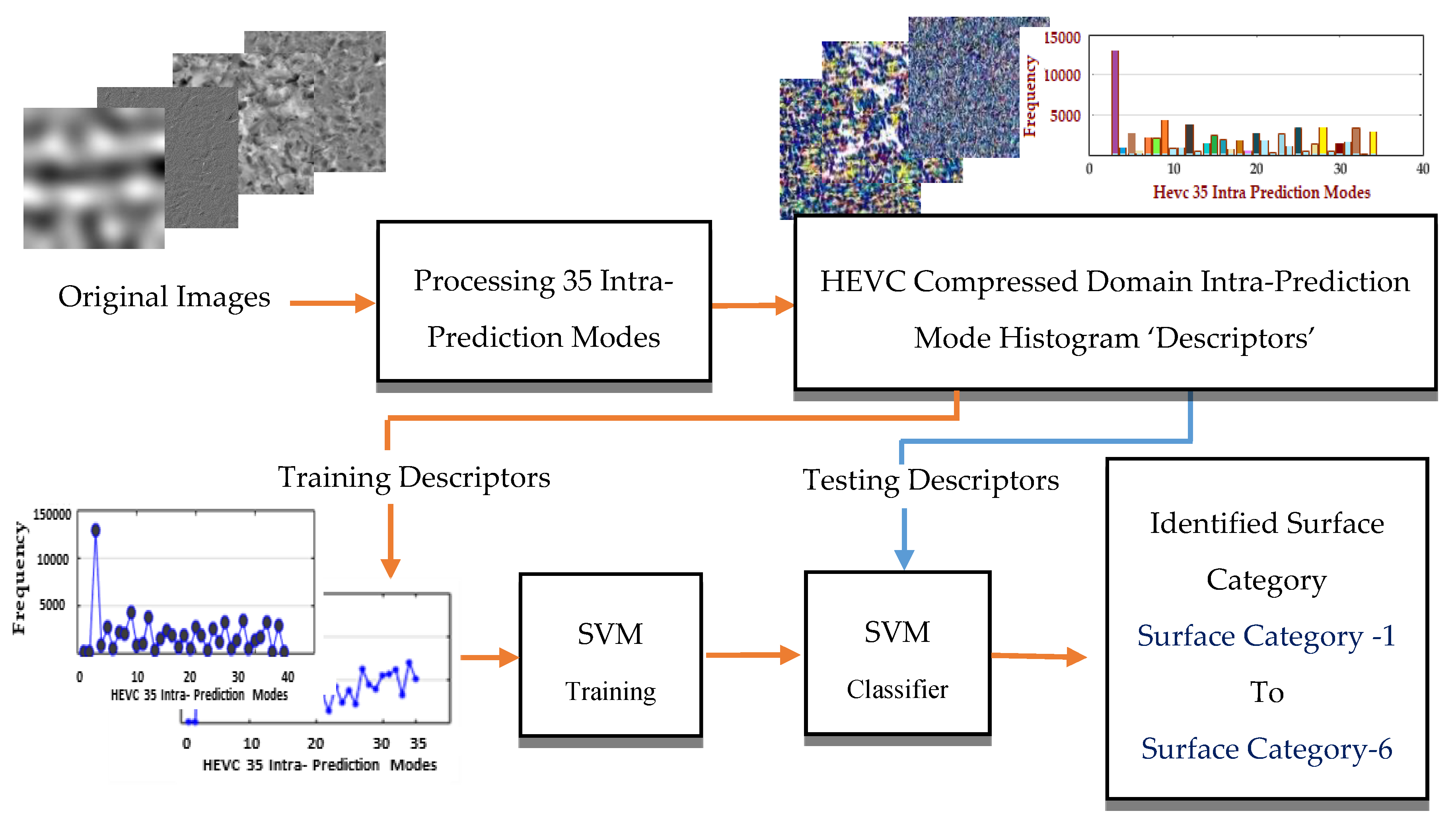
3.2. HEVC IPHM-Based Classification
- -
- Compress the entire topographical image database with HEVC lossless intra-prediction coding by computing the 35 intra-prediction modes for Prediction Units (PU) of size 4 × 4 pixels.
- -
- Search for the best prediction mode that minimizes the Sum of Absolute Difference (SAD). The selected mode indicates the relation between the pixels inside the Prediction Unit (PU) and the boundary neighbor pixels.
- -
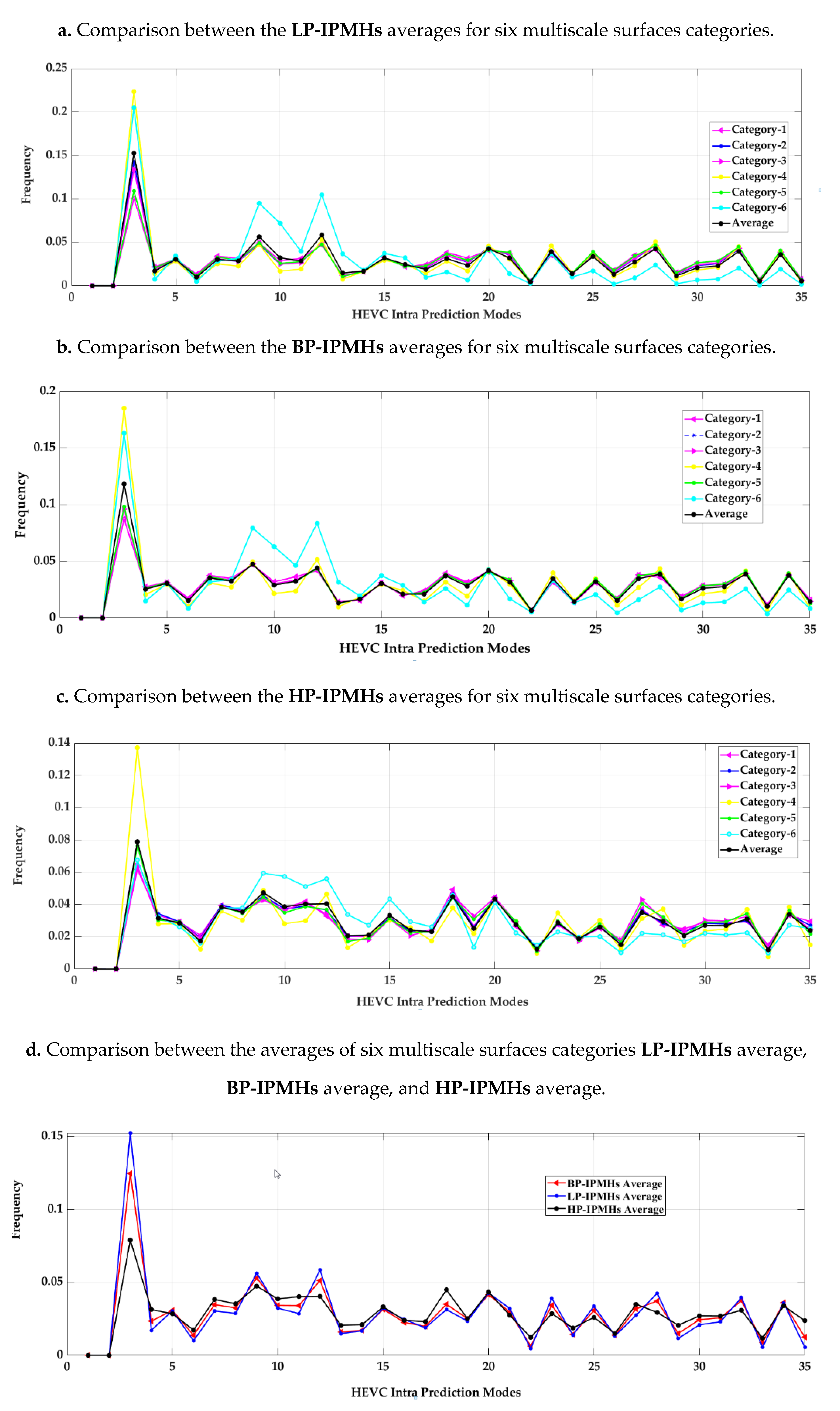
- Count the frequently utilized prediction modes to arrange each mode in one histogram bin as given by the following equation:where is the bin of the histogram for the mode (i). indicates the number of blocks in the coded picture which are predicted by mode (i).
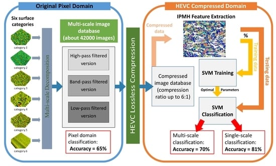
3.3. The Proposed Method
4. Simulation Results
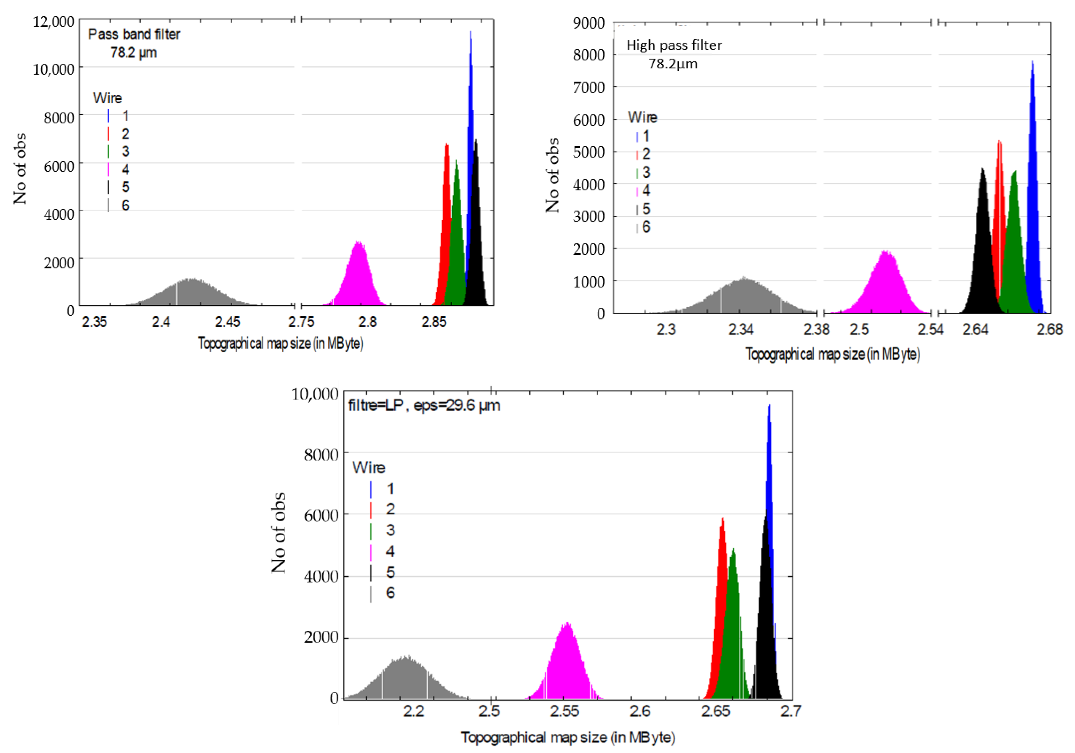
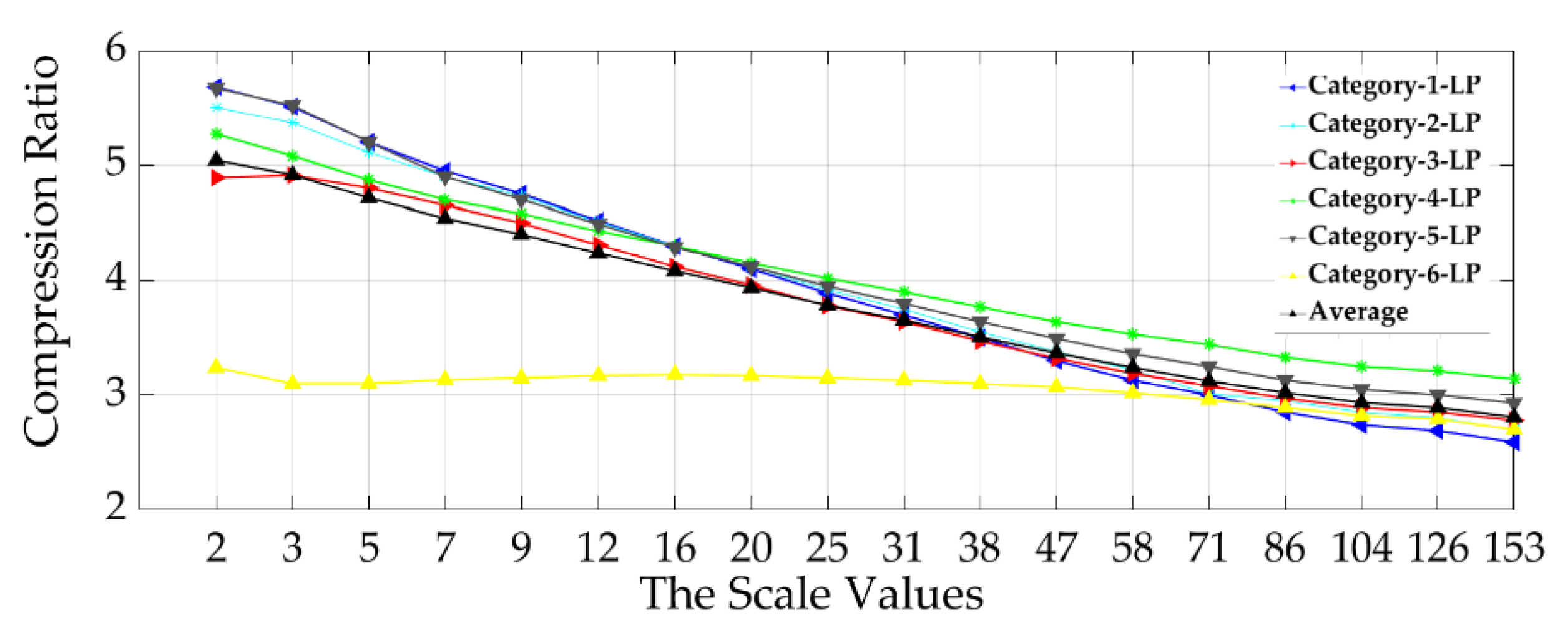
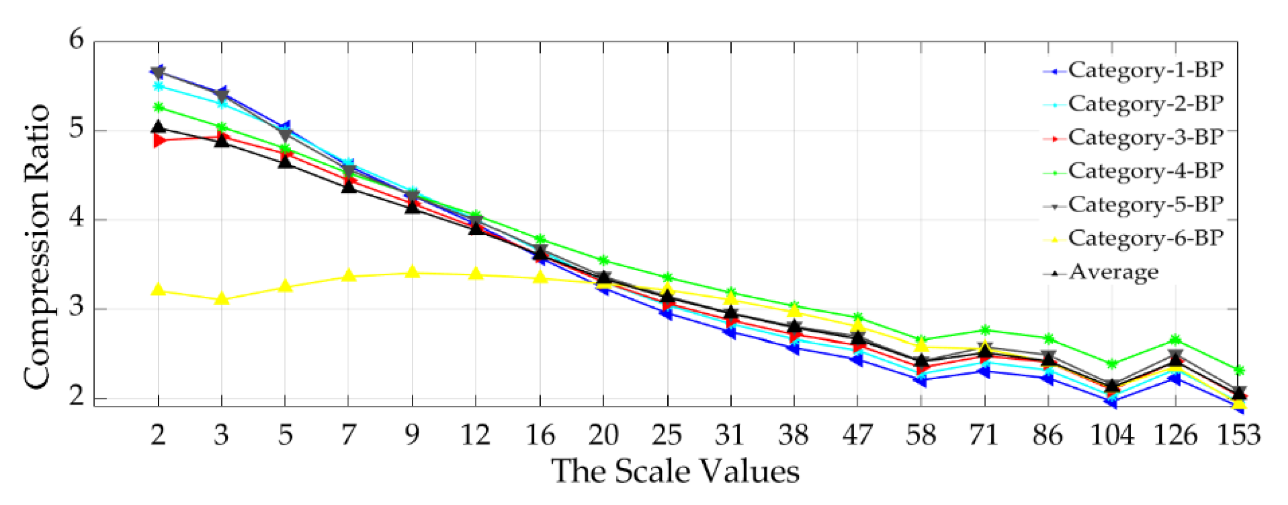
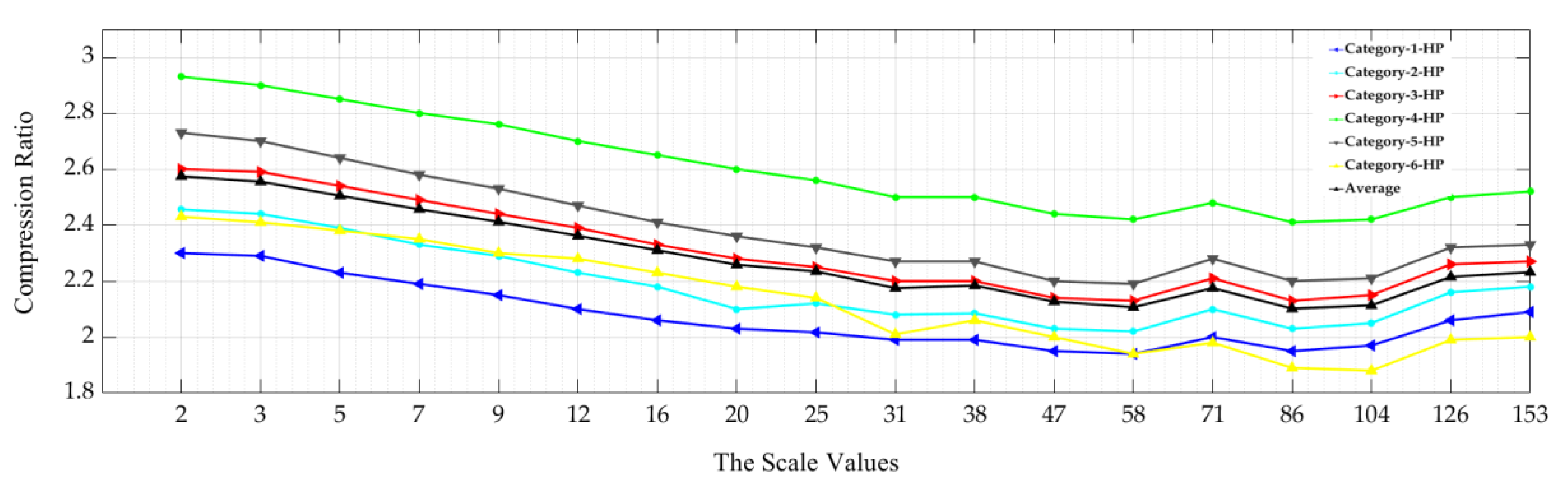
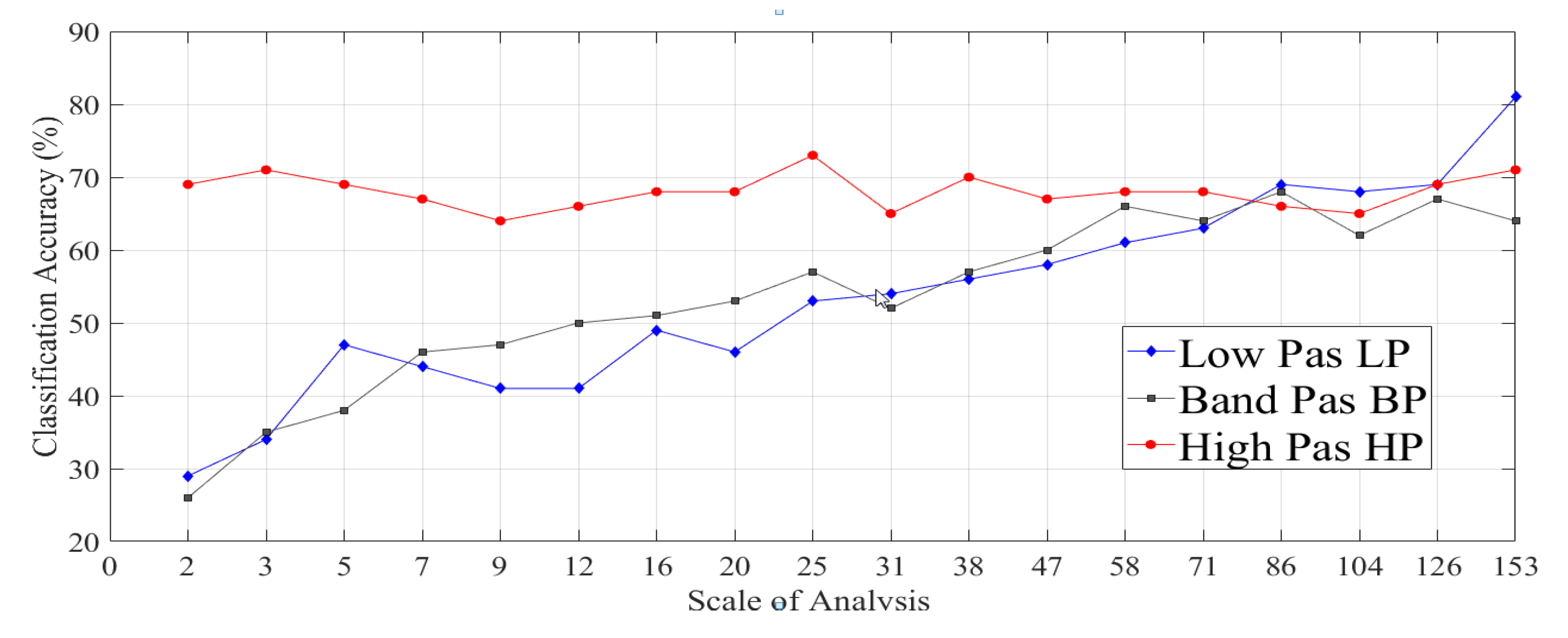
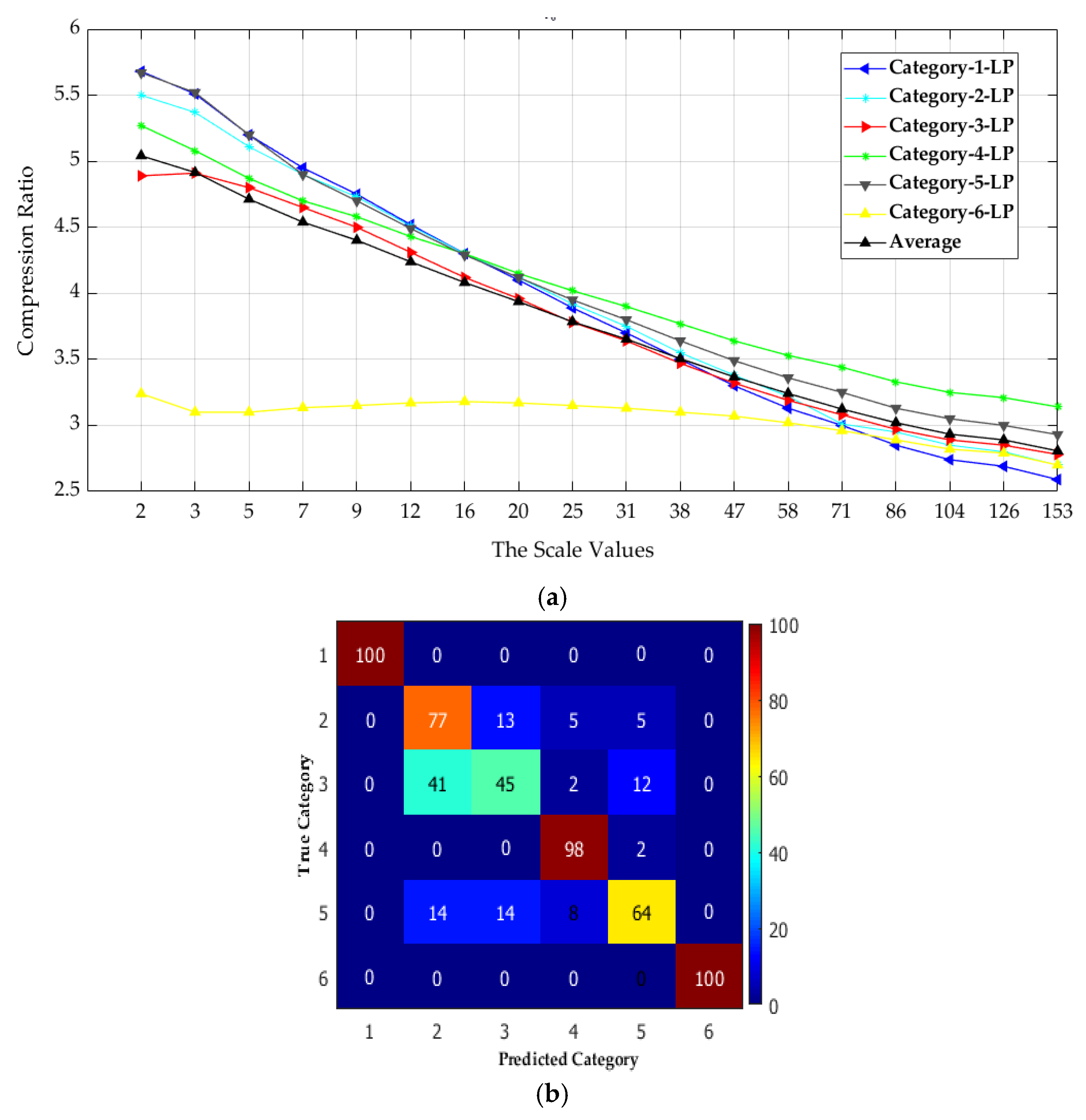
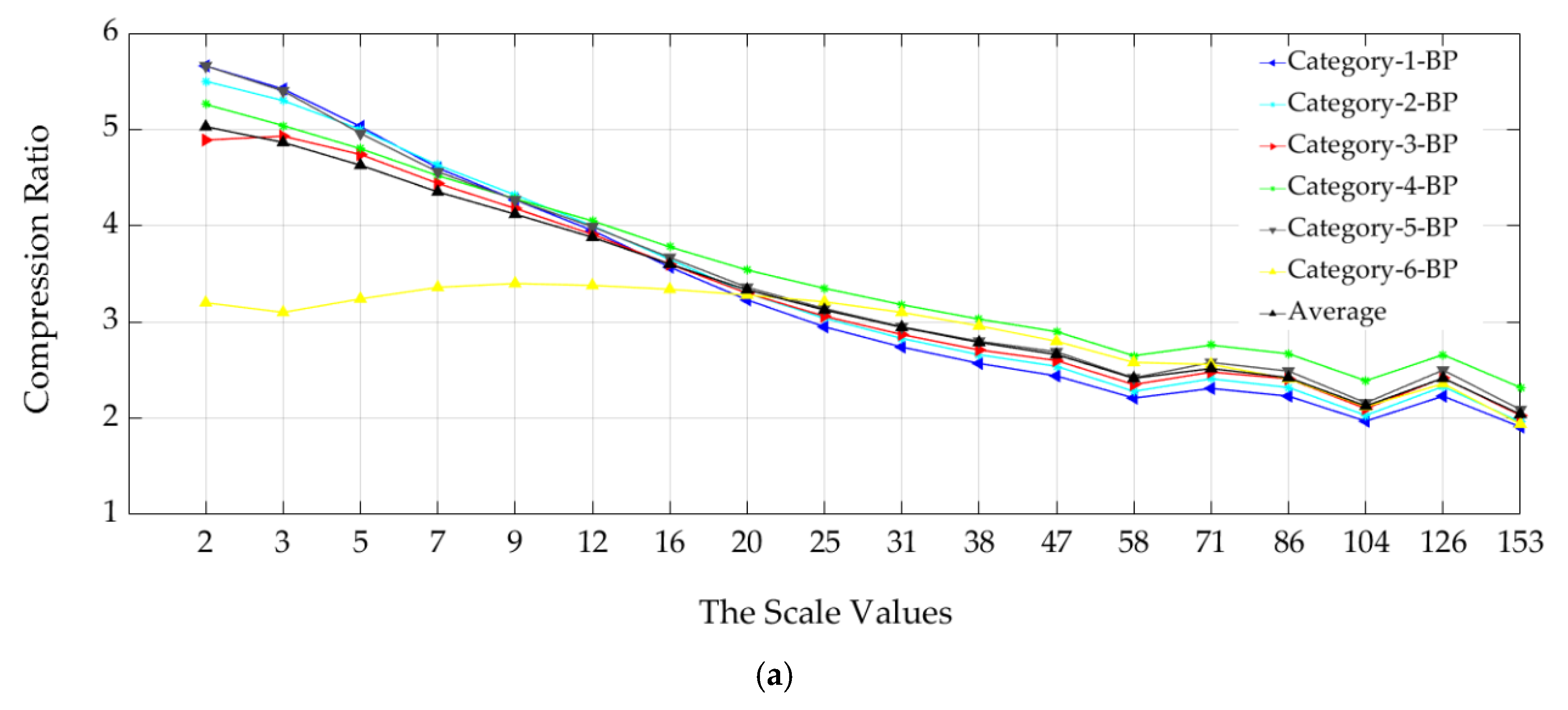
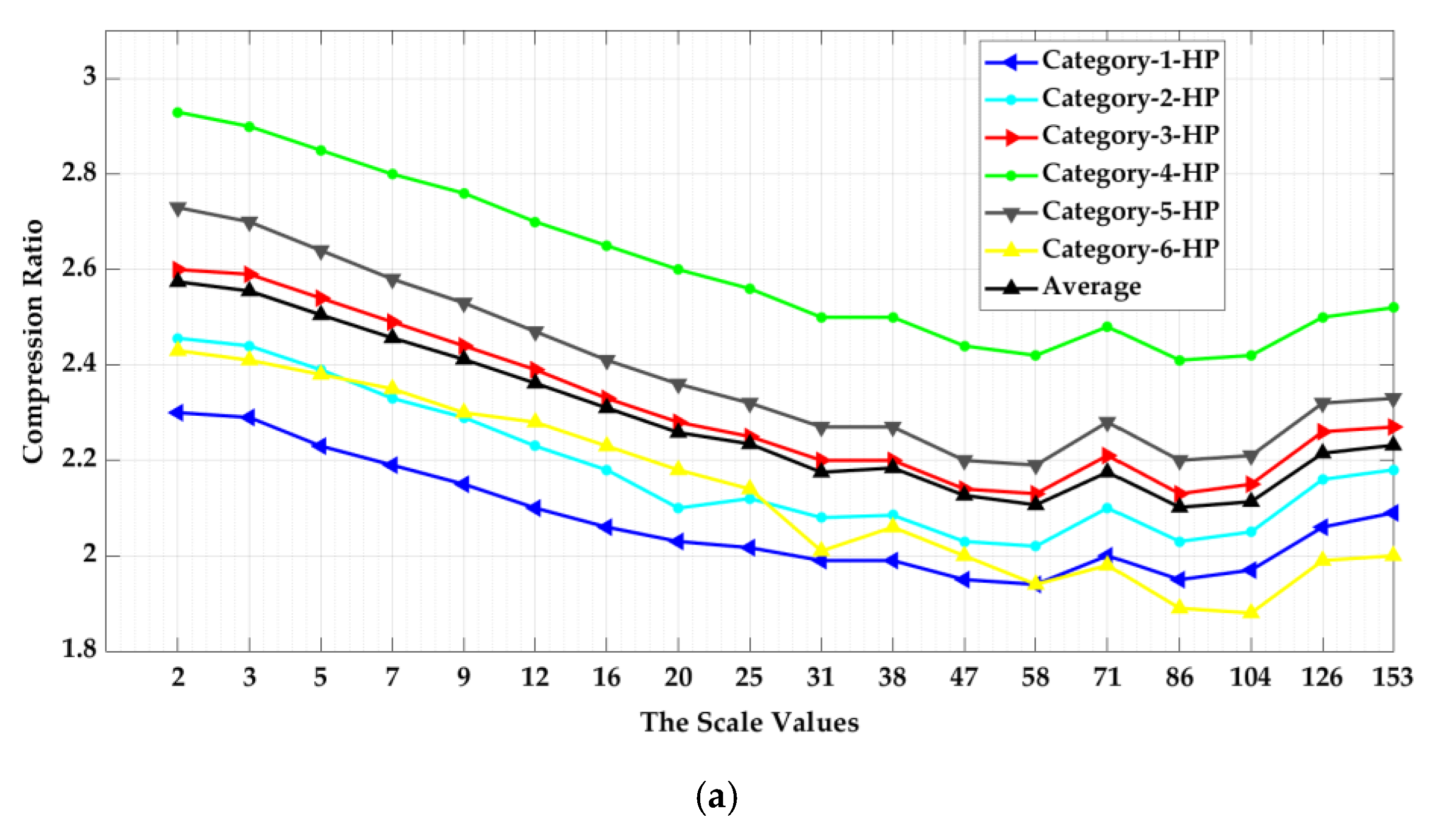
4.1. The Impact of Surface Topography Filtering Types on Achieved Compression Ratios
4.2. Evaluating IPMH as Texture Feature Descriptor
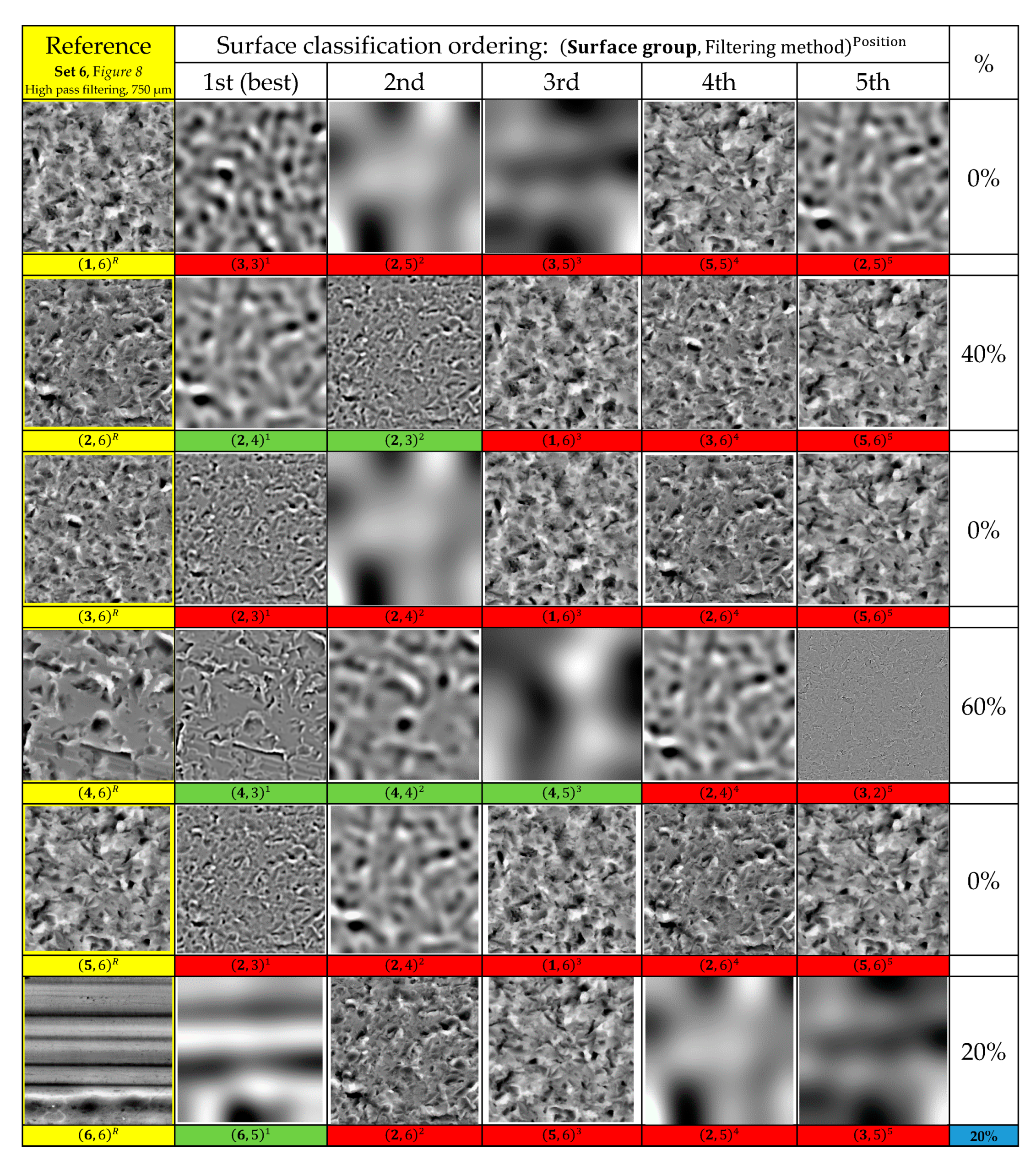
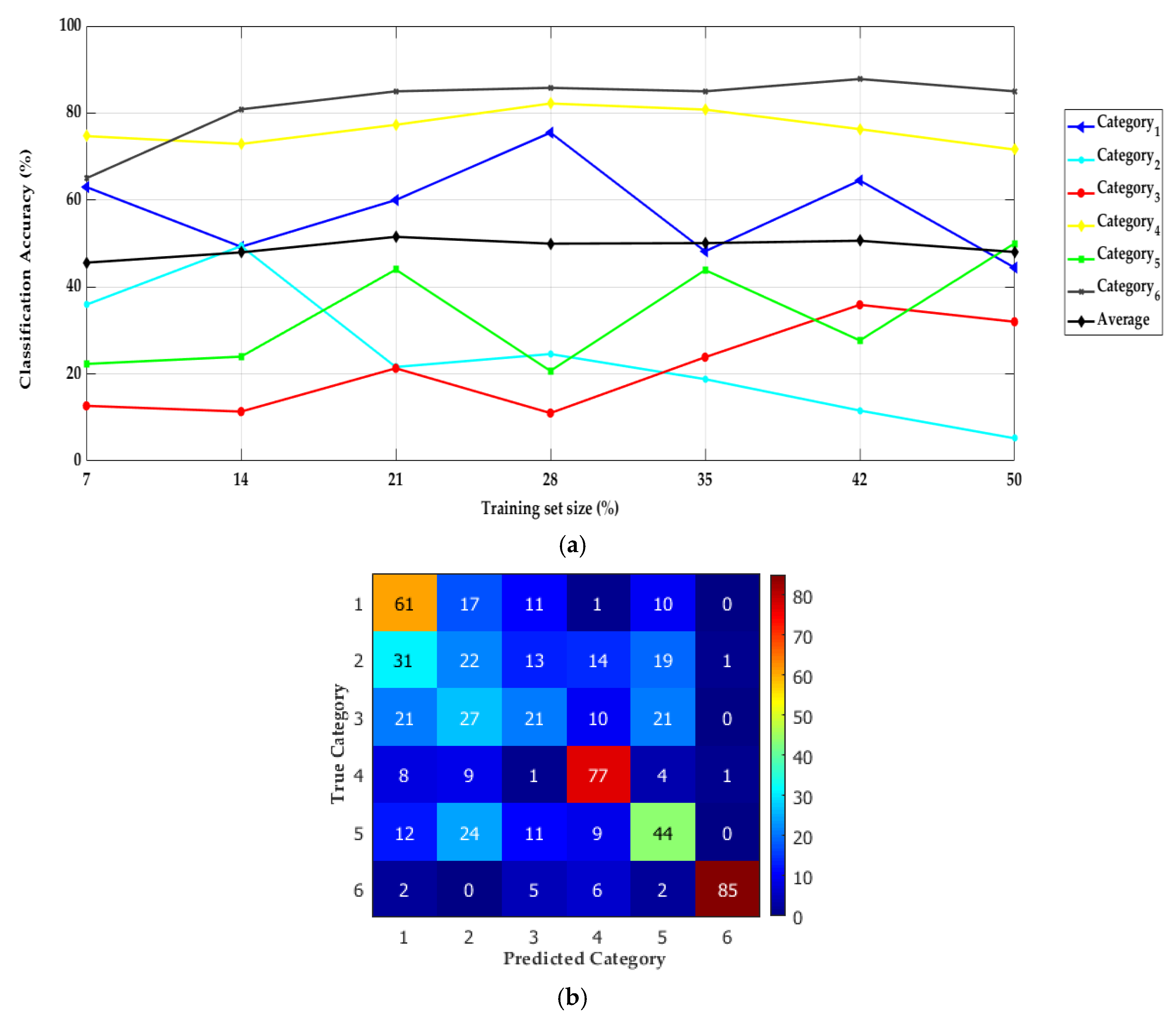
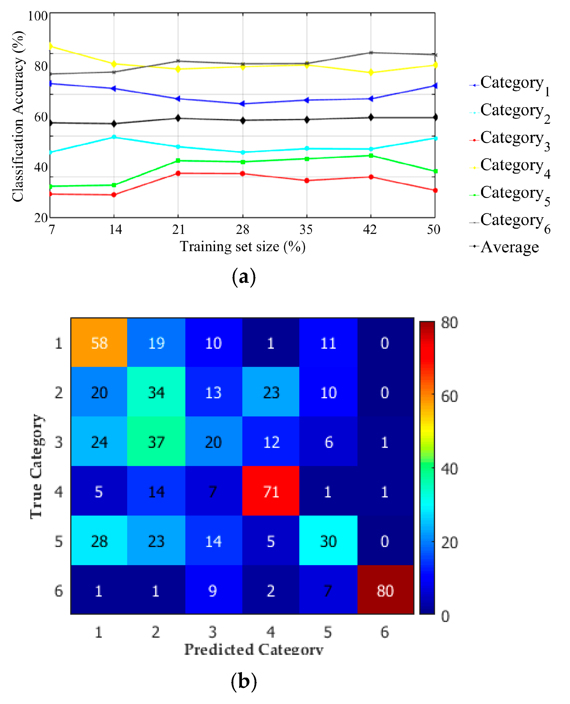
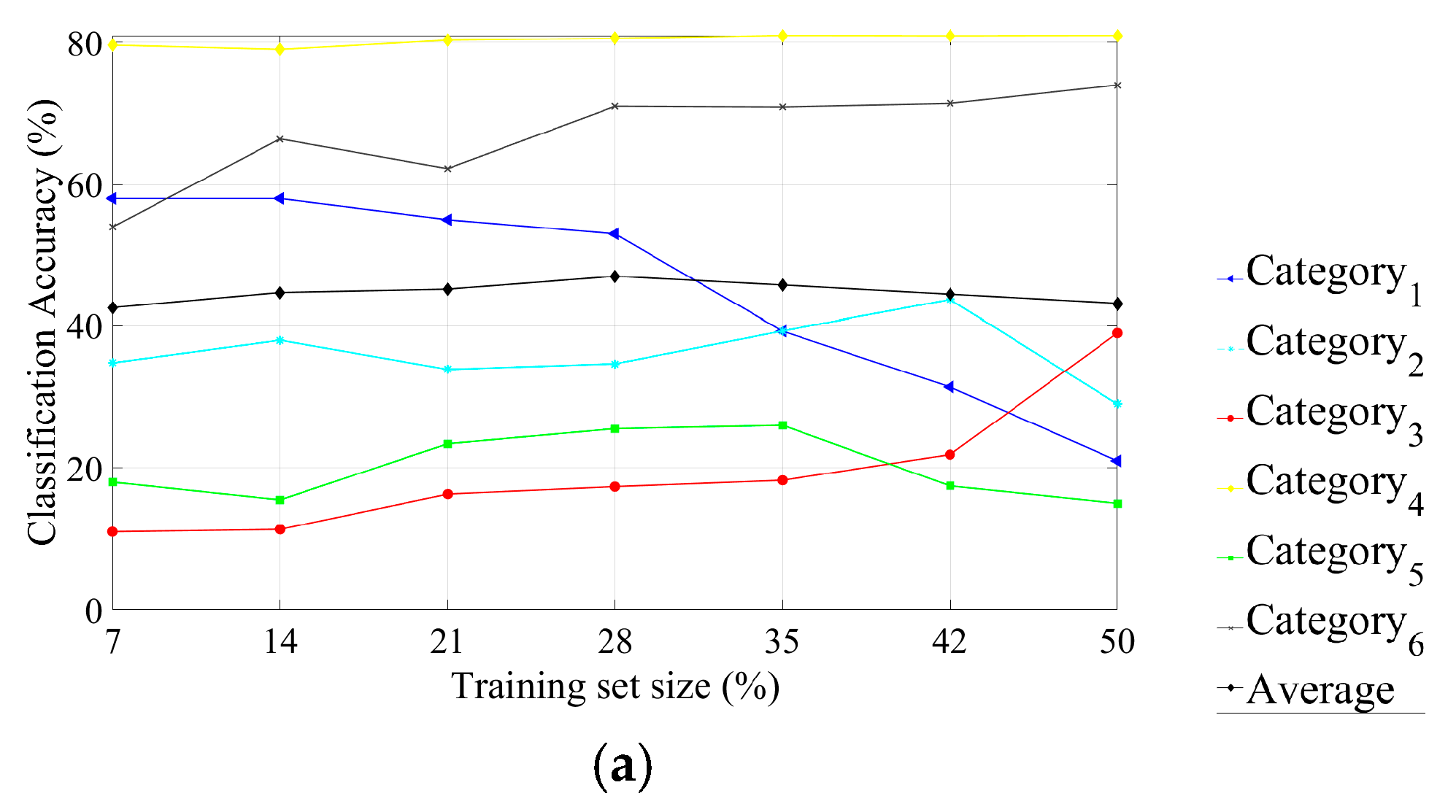
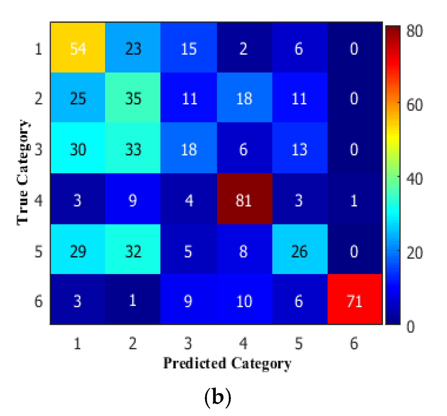
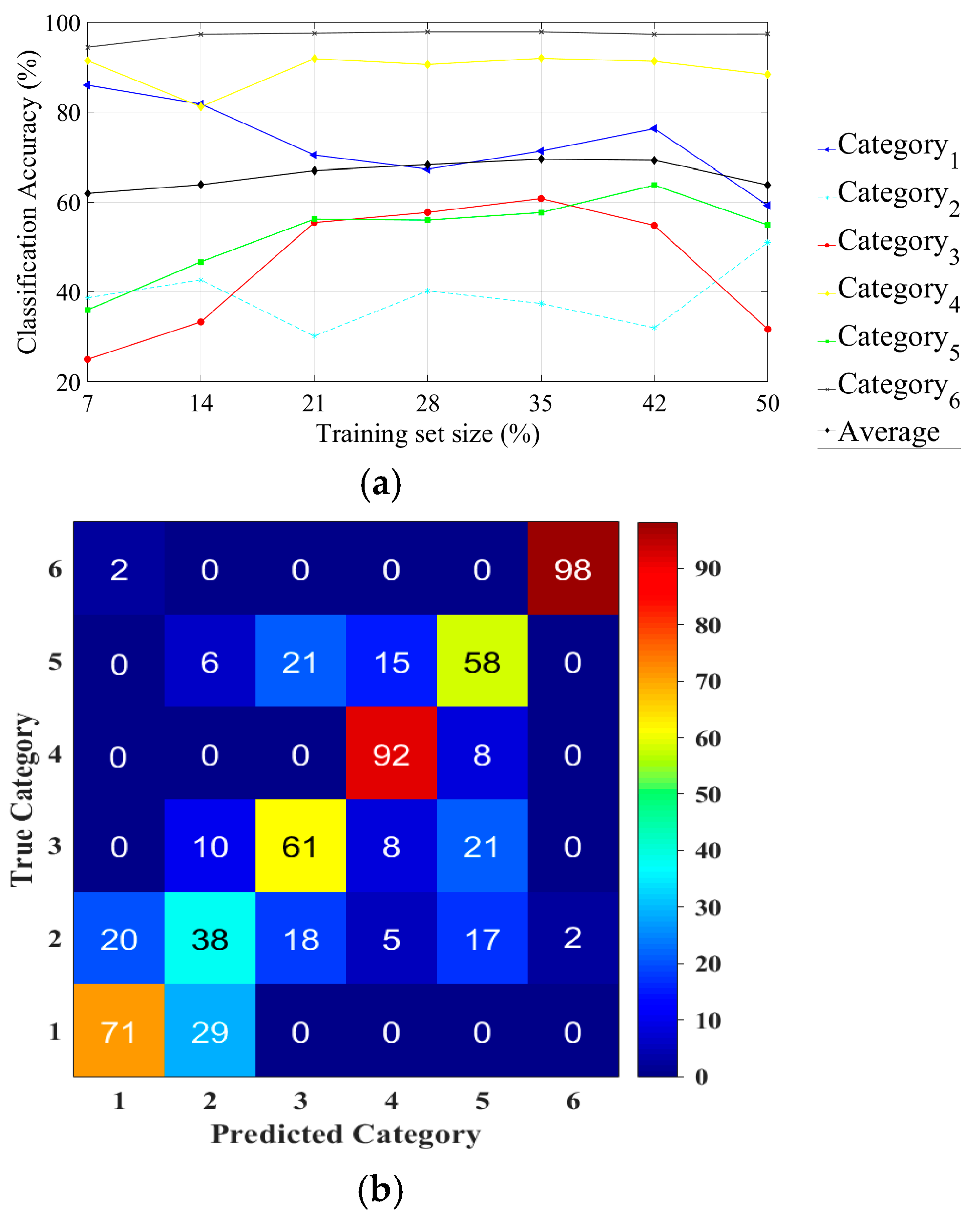
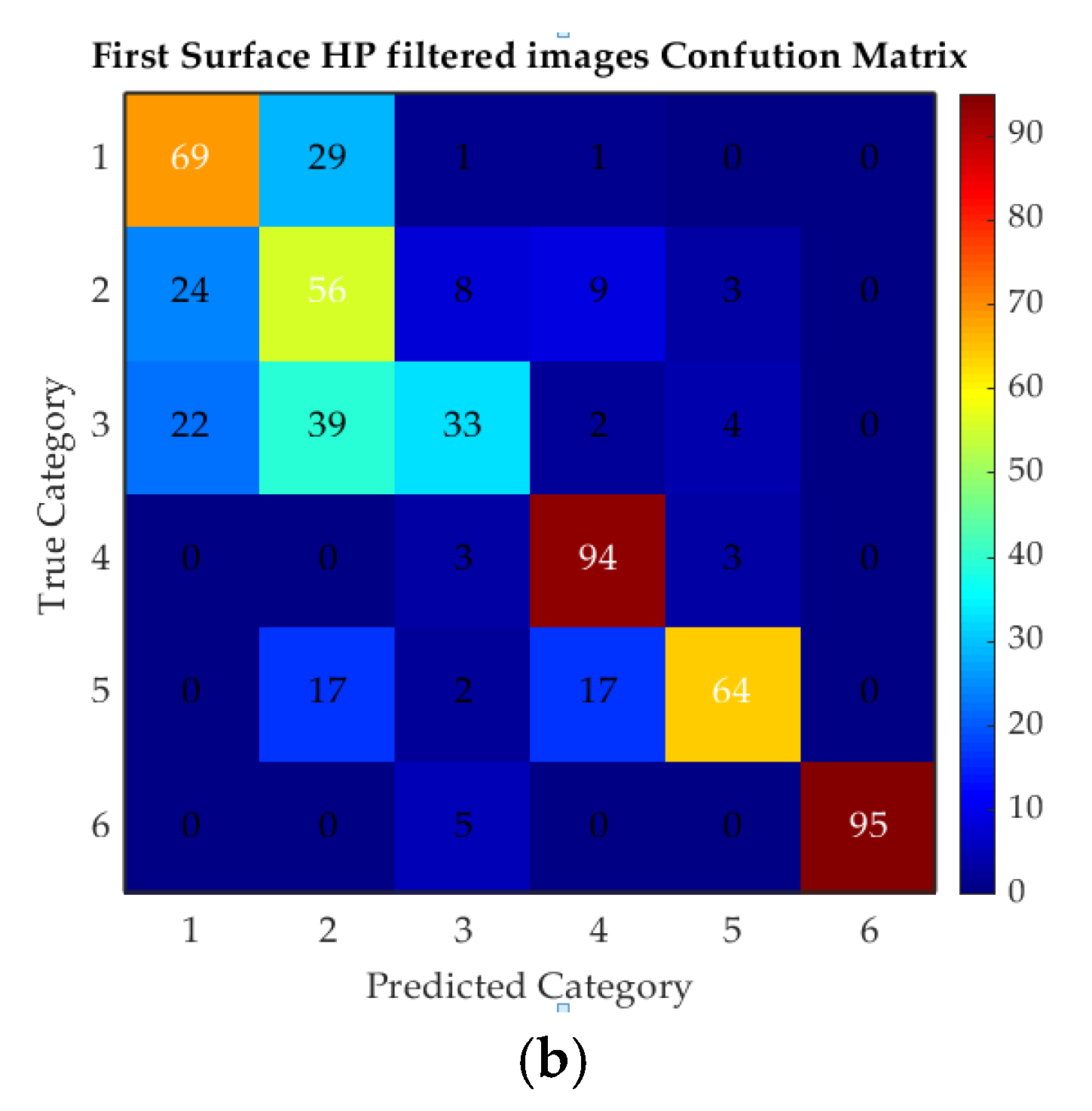
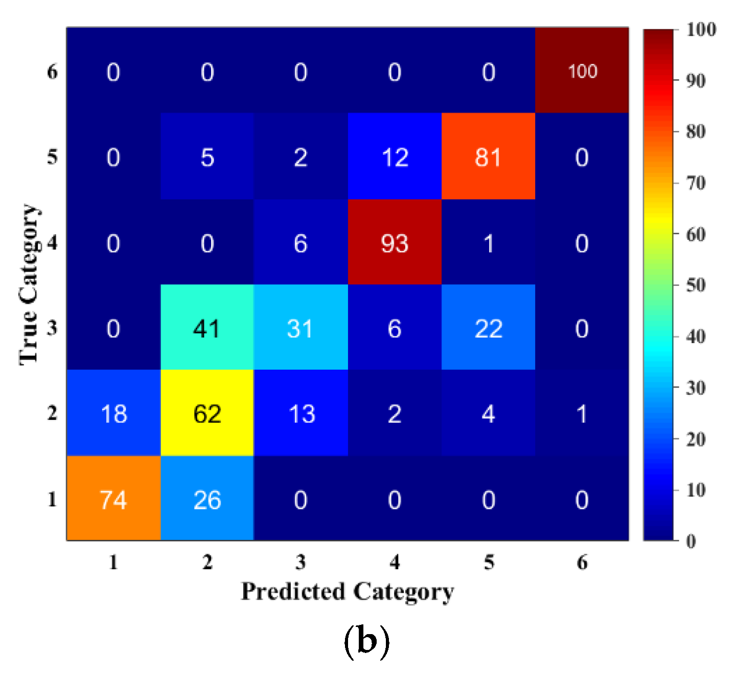
4.3. The Impact of Surface Topography Filtering Types on Topographical Images Classification Accuracy
- Case-1: the impact of considering the three-filtered image data sets together on the six surfaces categories’ classification performances.
- Case-2: the impact of each filter separately on the six surfaces categories’ classification performances.
- Case-3: the impact of each scale of analysis on the six surfaces categories’ classification performances.
4.4. The Impact of Scale of Analysis on Topographical Images Classification Accuracy
5. Conclusions
Author Contributions
Funding
Conflicts of Interest
Appendix A. Analysis by Conventional Methods


| ISO 25178 | |||
| Height Parameters | |||
| Sq | 6.42 | µm | Root-mean-square height |
| Ssk | −0.468 | Skewness | |
| Sku | 3.48 | Kurtosis | |
| Sp | 18.8 | µm | Maximum peak height |
| Sv | 29.0 | µm | Maximum pit height |
| Sz | 47.8 | µm | Maximum height |
| Sa | 5.04 | µm | Arithmetic mean height |
| Functional Parameters (Volume) | |||
| Vm | 0.243 | Material volume | |
| Vv | 8.02 | Void volume | |
| Vmp | 0.243 | Peak material volume | |
| Vmc | 5.68 | Core material volume | |
| Vvc | 7.13 | Core void volume | |
| Vvv | 0.889 | Pit void volume | |
| Functional Parameters (Stratified surfaces) | |||
| Sk | 15.5 | µm | Core roughness depth |
| Spk | 4.78 | µm | Reduced summit height |
| Svk | 8.12 | µm | Reduced valley depth |
| Smr1 | 8.62 | % | Upper bearing area |
| Smr2 | 87.1 | % | Lower bearing area |
| Spatial Parameters | |||
| Sal | 26.6 | µm | Auto correlation length |
| Str | 0.819 | Texture-aspect ratio | |
| Feature Parameters | |||
| Spd | 0.000312 | Density of peaks | |
| Spc | 0.306 | Arithmetic mean peak curvature | |
| S10z | 38.2 | µm | Ten-point height |
| S5p | 15.4 | µm | Five-point peak height |
| S5v | 22.7 | µm | Five-point pit height |
| Sda | 2333 | µm | Mean dale area |
| Sha | 3135 | µm | Mean hill area |
| Sdv | 1745 | µm | Mean dale volume |
| Shv | 1663 | µm | Mean hill volume |
| EUR 15178N | |||
| Hybrid Parameters | |||
| Sdq | 0.981 | Root-mean-square slope | |
| Sds | 0.00402 | Density of summits | |
| Ssc | 0.248 | Arithmetic mean summit curvature | |
| Sdr | 38.4 | % | Developed interfacial area |
| Sfd | 2.51 | Fractal dimension of the surface | |
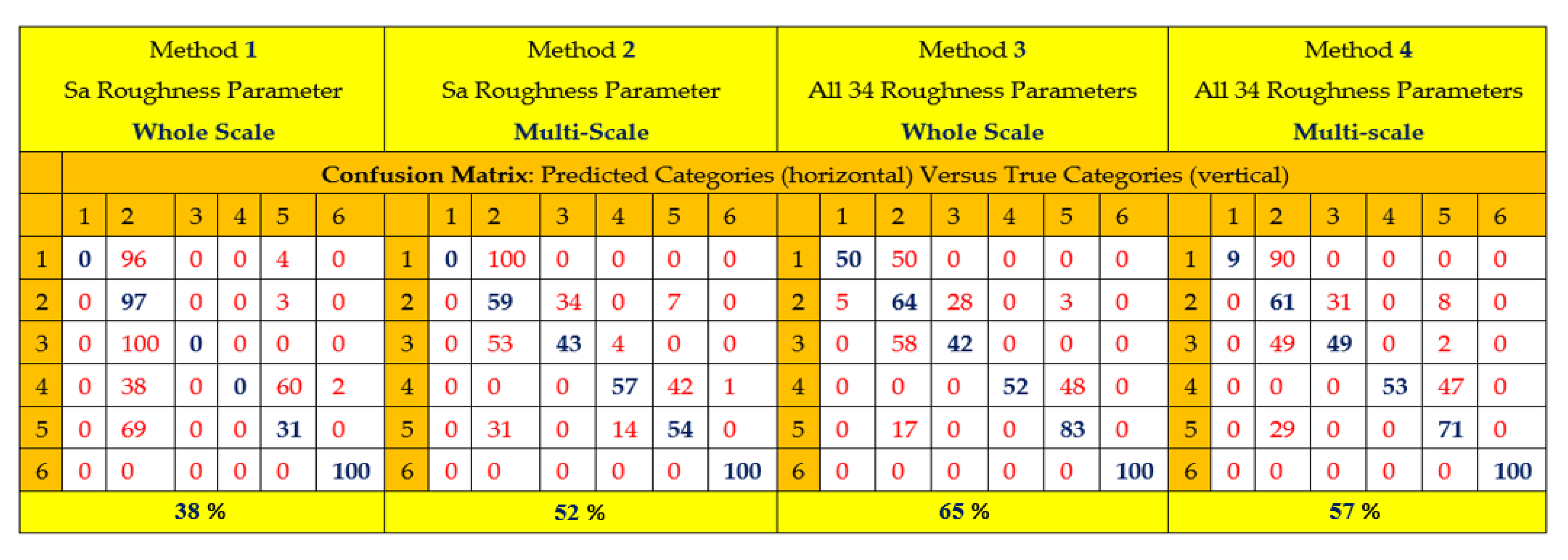
- Method 1. Sa Analyses. Sa is the arithmetic average value of roughness determined from deviations about the center plane. Sa is by far the most common roughness parameter, though this is often for historical reasons and not for particular merit, as the early roughness meters could only measure it. Whitehouse discusses the advantages of this parameter (robust and easy to understand) and the inconvenience (unable to characterize the skewness of the surface amplitude, i.e., difference of peaks and valleys, unable to characterize the size of peaks and valleys) [44]. The Sa is computed without filtering, i.e., at the whole scale. SVM classification is performed with this unique roughness parameter.
- Method 2. Sa Multiscale Analysis. As presented in Section 2.1, multiscale can be used to practice a multiscale decomposition and Sa roughness parameters are computed for all scales for the three Gaussian filters (pass band, low pass, and high pass). Giljean et al. [45] have shown that this multiscale analysis allows for the Sa roughness parameters to detect the size of the peaks and valleys, avoiding the main critic claimed by Whitehouse [44]. One obtains a set of parameters Sa (F,ε), where F is the filter and ε the scale length (cut off filter). From this set, SVM classification is processed.
- Method 3. Whole-scale analysis by a set of roughness parameters. Thirty-four Ri roughness parameters (see Table A1 for their descriptions) with i = {1, 2…,34} are computed without filtering, i.e., at the whole scale. Najjar et al. [46] has shown that the measure of functionality of a surface must be analyzed with the amplitude, spatial, and hybrid parameters to find the best one that characterizes the effect of roughness. They proposed a relevance function to classify the efficiency of roughness parameters based on variance analysis. One obtains a set of parameters Ri from which SVM classification is processed.
- Method 4. Multiscale analysis by a set of roughness parameters. Thirty-four Ri roughness parameters (see Table A1 for their descriptions) with i = {1, 2…,34} are computed for all scales for the three filters (pass band, low pass, and high pass). By analyzing all the roughness parameters of the GPS standard, Le Goic et. [10] showed that, with different types of filtering at different scales, ANOVA discriminates a wide range of tribological mechanisms by classification indexes based on databank of F values created from ANOVA [10]. One obtains a set of parameters Ri (F, ε), where F is the filter and ε is the scale length. From this set, SVM classification is processed.

References
- Ji, M.; Xu, J.; Chen, M.; EL Mansori, M. Enhanced hydrophilicity and tribology behavior of dental zirconia ceramics based on picosecond laser surface texturing. Ceram. Int. 2019, 46. [Google Scholar] [CrossRef]
- Brown, C.A.; Hansen, H.N.; Jiang, X.J.; Blateyron, F.; Berglund, J.; Senin, N.; Bartkowiak, T.; Dixon, B.; Le Goïc, G.; Quinsat, Y.; et al. Multiscale analyses and characterizations of surface topographies. CIRP Ann. 2018, 67, 839–862. [Google Scholar] [CrossRef]
- Ghosh, K.; Pandey, R. Fractal and multifractal analysis of in-doped ZnO thin films deposited on glass, ITO, and silicon substrates. Appl. Phys. A 2019, 125. [Google Scholar] [CrossRef]
- Hosseinabadi, S.; Karimi, Z.; Masoudi, A.A. Random deposition with surface relaxation model accompanied by long-range correlated noise. Phys. A Stat. Mech. Appl. 2020, 560, 125130. [Google Scholar] [CrossRef]
- Huaian, Y.; Xinjia, Z.; Le, T.; Yonglun, C.; Jie, Y. measuring grinding surface roughness based on singular value entropy of quaternion. Meas. Sci. Technol. 2020, 31, 115006. [Google Scholar] [CrossRef]
- Pahuja, R.; Ramulu, M. Characterization of surfaces generated in milling and abrasive water jet of CFRP using wavelet packet transform. IOP Conf. Ser. Mater. Sci. Eng. 2020, 842, 12001. [Google Scholar] [CrossRef]
- Bigerelle, M.; Iost, A. Characterisation of the diffusion states by data compression. Comput. Mater. Sci. 2002, 24, 133–138. [Google Scholar] [CrossRef]
- Zhang, A.; Wang, K.C.P. The fast prefix coding algorithm (FPCA) for 3D pavement surface data compression. Comput. Civ. Infrastruct. Eng. 2017, 32, 173–190. [Google Scholar] [CrossRef]
- Elkhuizen, W.S.; Callewaert, T.W.J.; Leonhardt, E.; Vandivere, A.; Song, Y.; Pont, S.C.; Geraedts, J.M.P.; Dik, J. Comparison of Three 3D scanning techniques for paintings, as applied to vermeer’s ‘girl with a pearl earring. Herit. Sci. 2019, 7, 89. [Google Scholar] [CrossRef]
- Le Goïc, G.; Bigerelle, M.; Samper, S.; Favrelière, H.; Pillet, M. multiscale roughness analysis of engineering surfaces: A comparison of methods for the investigation of functional correlations. Mech. Syst. Signal Process. 2016, 66–67, 437–457. [Google Scholar] [CrossRef]
- Mistry, Y.; Ingole, D.T.; Ingole, M.D. Content based image retrieval using hybrid features and various distance metric. J. Electr. Syst. Inf. Technol. 2017. [Google Scholar] [CrossRef]
- Mehrabi, M.; Zargari, F.; Ghanbari, M. compressed domain content based retrieval using H.264 DC-pictures. Multimed. Tools Appl. 2012, 60, 443–453. [Google Scholar] [CrossRef]
- Rahmani, F.; Zargari, F. Temporal feature vector for video analysis and retrieval in high efficiency video coding compressed domain. Electron. Lett. 2018, 54, 294–295. [Google Scholar] [CrossRef]
- Zargari, F.; Rahmani, F. Visual information retrieval in HEVC compressed domain. In Proceedings of the 23rd Iranian Conference on Electrical Engineering, Tehran, Iran, 10–14 May 2015; pp. 793–798. [Google Scholar] [CrossRef]
- Rahmani, F.; Zargari, F. Compressed domain visual information retrieval based on I-Frames in HEVC. Multimed. Tools Appl. 2017, 76, 7283–7300. [Google Scholar] [CrossRef]
- Yamaghani, M.; Zargari, F. Classification and retrieval of radiology images in H.264/AVC compressed domain. Signal Image Video Process. 2017, 11, 573–580. [Google Scholar] [CrossRef]
- Zargari, F.; Mehrabi, M.; Ghanbari, M. Compressed domain texture based visual information retrieval method for I-Frame coded pictures. IEEE Trans. Consum. Electron. 2010, 56, 728–736. [Google Scholar] [CrossRef]
- Yamghani, A.R.; Zargari, F. Compressed domain video abstraction based on I-Frame of HEVC coded videos. Circuits Syst. Signal Process. 2019, 38, 1695–1716. [Google Scholar] [CrossRef]
- Zygo Corporation. NewView 7200 & 7300 Operating Manual, OMP-0536, Rev. E, ed.; Zygo Corporation: Middlefield, CT, USA, 2011. [Google Scholar]
- Yoshizawa, T. Handbook of Optical Metrology Principles and Applications, 2nd ed.; CRC Press: Boca Raton, FL, USA, 2015. [Google Scholar] [CrossRef]
- Bigerelle, M.; Guillemot, G.; Khawaja, Z.; El Mansori, M.; Antoni, J. Relevance of wavelet shape selection in a complex signal. Mech. Syst. Signal Process. 2013, 41, 14–33. [Google Scholar] [CrossRef]
- Bigerelle, M.; Abdel-Aal, H.A.; Iost, A. Relation between entropy, free energy and computational energy. Int. J. Mater. Prod. Technol. 2010, 38, 35–43. [Google Scholar] [CrossRef]
- Bigerelle, M.; Haidara, H.; Van Gorp, A. Monte carlo simulation of gold nano-colloids aggregation morphologies on a heterogeneous surface. Mater. Sci. Eng. C 2006, 26, 1111–1116. [Google Scholar] [CrossRef]
- Bigerelle, M.; Dalla-Costa, M.; Najjar, D. Multiscale similarity characterization of abraded surfaces. Proc. Inst. Mech. Eng. Part B J. Eng. Manuf. 2007, 221, 1473–1482. [Google Scholar] [CrossRef]
- Dalla Costa, M.; Bigerelle, M.; Najjar, D. A new methodology for quantifying the multi-scale similarity of images. Microelectron Eng. 2007, 84, 424–430. [Google Scholar] [CrossRef]
- Lemesle, J.; Robache, F.; Le Goic, G.; Mansouri, A.; Brown, C.A.; Bigerelle, M. Surface reflectance: An optical method for multiscale curvature characterization of wear on ceramic-metal composites. Materials 2020, 13, 1024. [Google Scholar] [CrossRef] [PubMed] [Green Version]
- Sullivan, G.J.; Ohm, J.; Han, W.; Wiegand, T. Overview of the high efficiency video coding (HEVC) standard. IEEE Trans. Circuits Syst. Video Technol. 2012, 22, 1649–1668. [Google Scholar] [CrossRef]
- Sze, V.; Budagavi, M.; Sullivan, G.J. High Efficiency Video Coding (HEVC): Algorithms and Architectures, 1st ed.; Springer Publishing Company, Incorporated: Cham, Switzerland, 2014. [Google Scholar] [CrossRef]
- Li, J.; Li, B.; Xu, J.; Xiong, R.; Gao, W. Fully connected network-based intra prediction for image coding. IEEE Trans. Image Process. 2018, 27, 3236–3247. [Google Scholar] [CrossRef]
- Flynn, D.; Marpe, D.; Naccari, M.; Nguyen, T.; Rosewarne, C.; Sharman, K.; Sole, J.; Xu, J. Overview of the range extensions for the HEVC Standard: Tools, profiles, and performance. IEEE Trans. Circuits Syst. Video Technol. 2016, 26, 4–19. [Google Scholar] [CrossRef]
- Humeau-heurtier, A. Texture feature extraction methods: A survey. IEEE Access 2019, 7, 8975–9000. [Google Scholar] [CrossRef]
- Faust, O.; Acharya, U.R.; Meiburger, K.M.; Molinari, F.; Koh, J.E.W.; Yeong, C.H.; Kongmebhol, P.; Ng, K.H. Comparative assessment of texture features for the identification of cancer in ultrasound images: A review. Biocybern. Biomed. Eng. 2018, 38, 275–296. [Google Scholar] [CrossRef] [Green Version]
- Lan, Z. Study on multi-scale window determination for GLCM texture description in high-resolution remote sensing image geo-analysis supported by GIS and domain knowledge. Int. J. Geo Inf. 2018, 7, 175. [Google Scholar] [CrossRef] [Green Version]
- Pérez-Barnuevo, L. Automated recognition of drill core textures: A geometallurgical tool for mineral processing prediction. Miner. Eng. 2017, 118. [Google Scholar] [CrossRef]
- García-ordás, M.T.; Alegre-gutiérrez, E.; Alaiz-rodríguez, R.; González-castro, V. Tool wear monitoring using an online, automatic and low cost system based on local texture. Mech. Syst. Signal Process. 2018, 112, 98–112. [Google Scholar] [CrossRef]
- Binias, B.; Myszor, D. A Machine learning approach to the detection of pilot’ s reaction to unexpected events based on EEG signals. Comput. Intell. Neurosci. 2018, 14, 1–9. [Google Scholar] [CrossRef] [Green Version]
- Zhang, X.; Cui, J.; Wang, W.; Lin, C. A study for texture feature extraction of high-resolution satellite images based on a direction measure and gray level co-occurrence matrix fusion algorithm. Sensors 2017, 17, 1474. [Google Scholar] [CrossRef] [PubMed] [Green Version]
- Gao, L.; Ye, M.; Wu, C. Cancer classification based on support vector machine optimized by particle swarm optimization. Molecules 2017, 22, 2086. [Google Scholar] [CrossRef] [PubMed] [Green Version]
- Zeng, N.; Qiu, H.; Wang, Z.; Liu, W.; Zhang, H.; Li, Y. A new switching-delayed-PSO-based optimized SVM algorithm for diagnosis of alzheimer’s disease. Neurocomputing 2018, 320, 195–202. [Google Scholar] [CrossRef]
- Machine, V. A novel method for the recognition of air visibility level based on the optimal binary tree support vector machine. Atmosphere 2018, 9, 481. [Google Scholar] [CrossRef] [Green Version]
- Ortegon, J.; Ledesma-Alonso, R.; Barbosa, R.; Castillo, J.; Castillo Atoche, A. Material phase classification by means of support vector machines. Comput. Mater. Sci. 2017, 148, 336–342. [Google Scholar] [CrossRef] [Green Version]
- Ben-david, S.; Shalev-Shwartz, S. Understanding Machine Learning: From Theory to Algorithms; Cambridge University Press: Cambridge, UK, 2014. [Google Scholar]
- Zhang, Z.; Chen, H.; Xu, Y.; Zhong, J.; Lv, N.; Chen, S. Multisensor-based real-time quality monitoring by means of feature extraction, selection and modeling for Al alloy in arc welding. Mech. Syst. Signal Process. 2015, 61, 151–165. [Google Scholar] [CrossRef]
- Whitehouse, D.J. Handbook of Surface Metrology, 1st ed.; Institute of Physics Publishing for Rank Taylor Hobson Co., Bristol: London, UK, 1994. [Google Scholar]
- Giljean, S.; Najjar, D.; Bigerelle, M.; Alain, I. Multiscale analysis of abrasion damage on stainless steel. Surf. Eng. 2008, 24, 8–17. [Google Scholar] [CrossRef]
- Najjar, D.; Bigerelle, M.; Iost, A. The Computer-based bootstrap method as a tool to select a relevant surface roughness parameter. Wear 2003, 254, 450–460. [Google Scholar] [CrossRef]


| Lens Magnification | 50× |
|---|---|
| Map resolution (pixel) | 640 × 480 |
| Number of stitches | 5 × 27, 20% overlapping |
| Final investigated area (mm) | 6.16 × 0.89 |
| Lateral resolution (µm) | 0.44 |
| Final resolution (pixel) | 13,952 × 2014 |
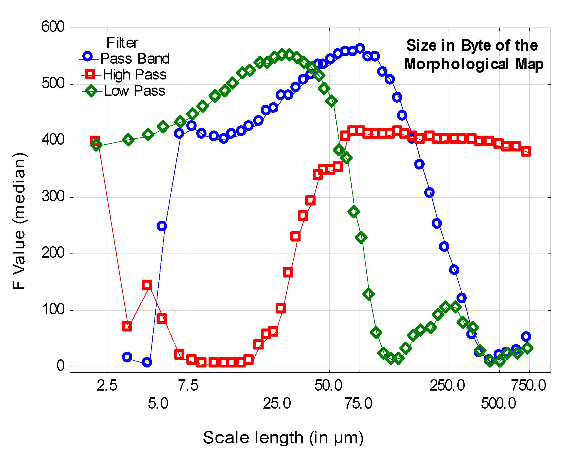
| Filter | Scale | Fmean | F5th | F50th | F95th |
|---|---|---|---|---|---|
| Band pass | 78.2 | 566 | 441 | 558 | 721 |
| High pass | 78.2 | 418 | 334 | 414 | 515 |
| Low pass | 29.6 | 552 | 454 | 548 | 666 |
| Coding Options | Chosen Parameter |
|---|---|
| Encoder version | 16.12 |
| Profile | Main-still-picture |
| Internal bit depth | 8 |
| Frames to be encoded | 1 |
| Max CU width | 16 |
| Max CU height | 16 |
| GOP | 1 |
| Search range | 64 |
| Quantization parameter | 0 |
| Transform skip | Disabled |
| Transform skip Fast | Disabled |
| Deblocking filter | 0 |
| Sample adaptive offset | Disabled |
| Trans quant bypass ena | 0 |
| CU Trans quant bypass | 0 |
Publisher’s Note: MDPI stays neutral with regard to jurisdictional claims in published maps and institutional affiliations. |
© 2020 by the authors. Licensee MDPI, Basel, Switzerland. This article is an open access article distributed under the terms and conditions of the Creative Commons Attribution (CC BY) license (http://creativecommons.org/licenses/by/4.0/).
Share and Cite
Eseholi, T.; Coudoux, F.-X.; Corlay, P.; Sadli, R.; Bigerelle, M. A Multiscale Topographical Analysis Based on Morphological Information: The HEVC Multiscale Decomposition. Materials 2020, 13, 5582. https://doi.org/10.3390/ma13235582
Eseholi T, Coudoux F-X, Corlay P, Sadli R, Bigerelle M. A Multiscale Topographical Analysis Based on Morphological Information: The HEVC Multiscale Decomposition. Materials. 2020; 13(23):5582. https://doi.org/10.3390/ma13235582
Chicago/Turabian StyleEseholi, Tarek, François-Xavier Coudoux, Patrick Corlay, Rahmad Sadli, and Maxence Bigerelle. 2020. "A Multiscale Topographical Analysis Based on Morphological Information: The HEVC Multiscale Decomposition" Materials 13, no. 23: 5582. https://doi.org/10.3390/ma13235582