Mixture Optimization of Recycled Aggregate Concrete Using Hybrid Machine Learning Model


Abstract
:1. Introduction
1.1. Related Work
1.2. Research Significance
2. Machine Learning Basis
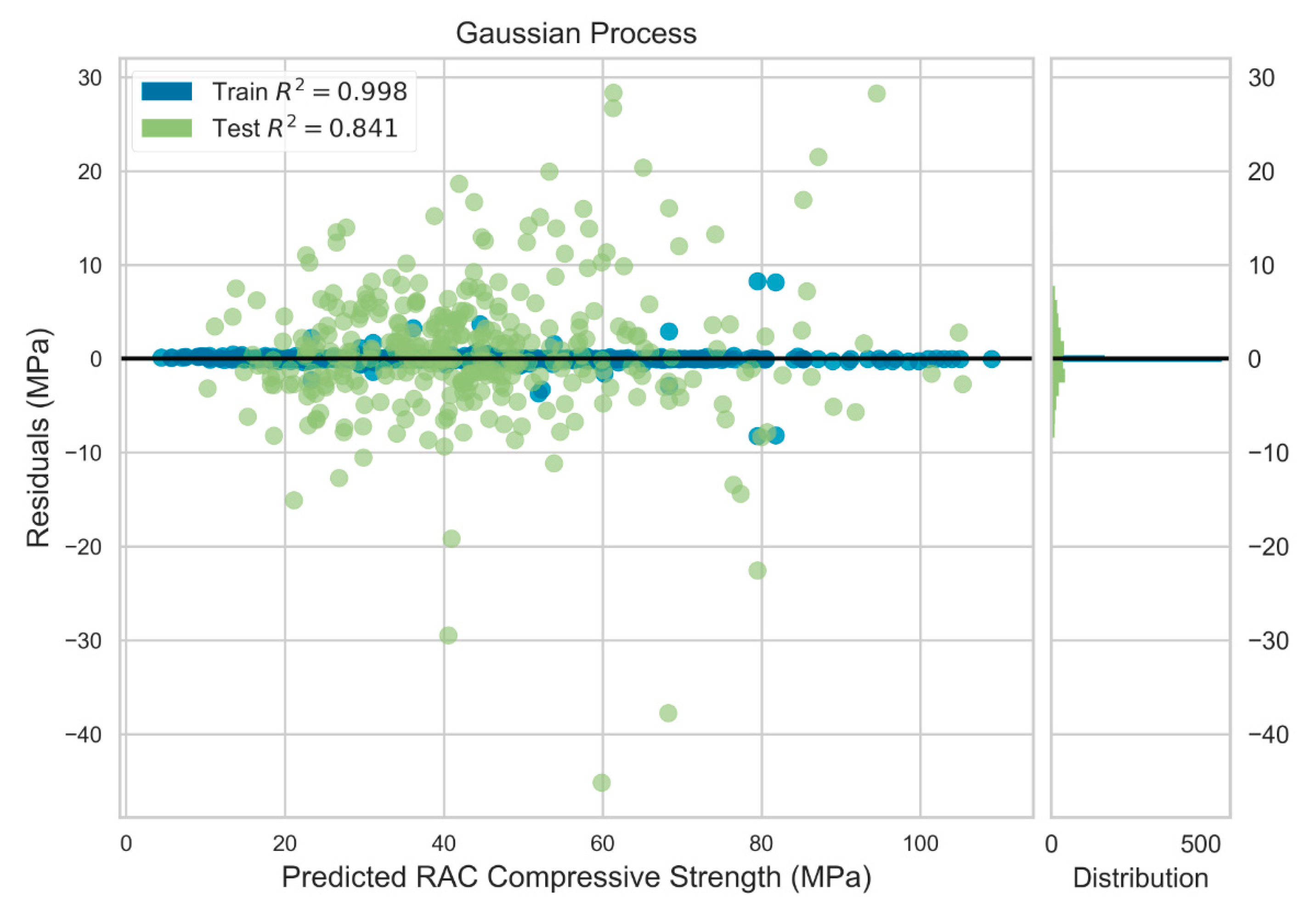
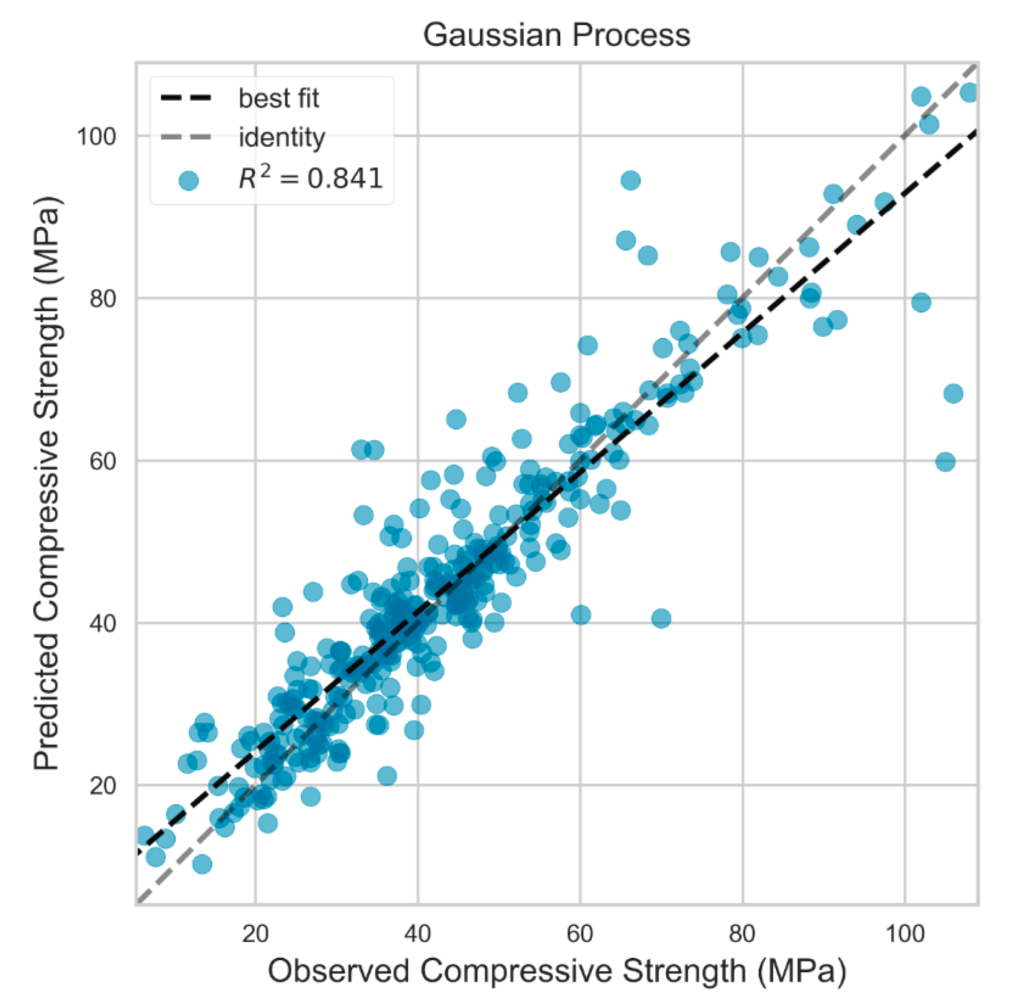
2.1. Gaussian Processes
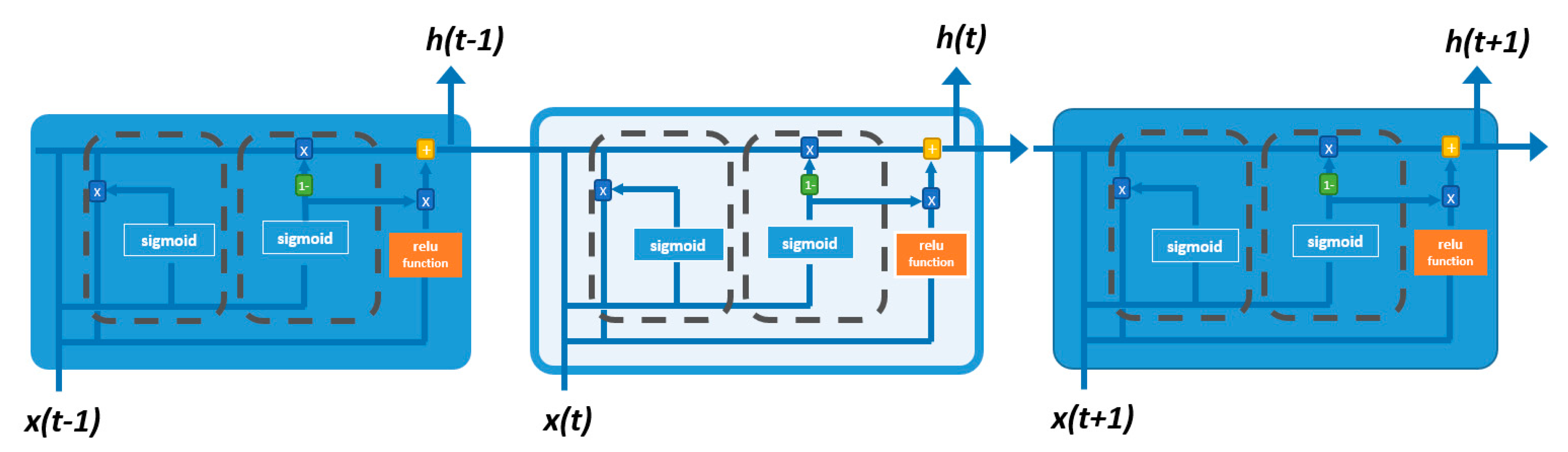
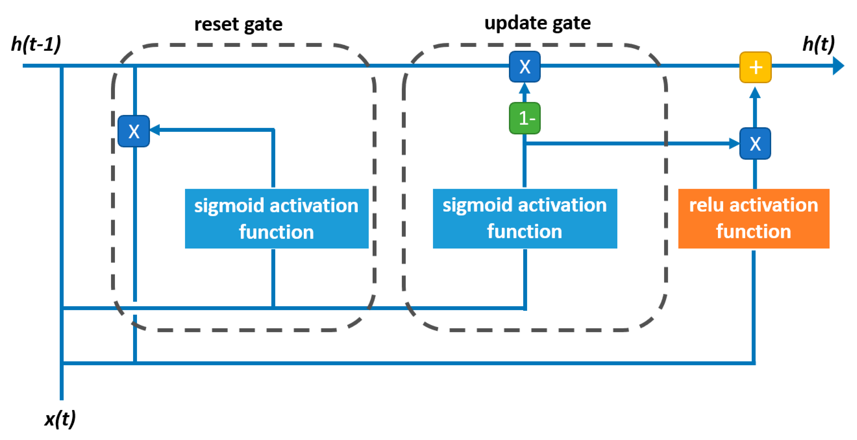
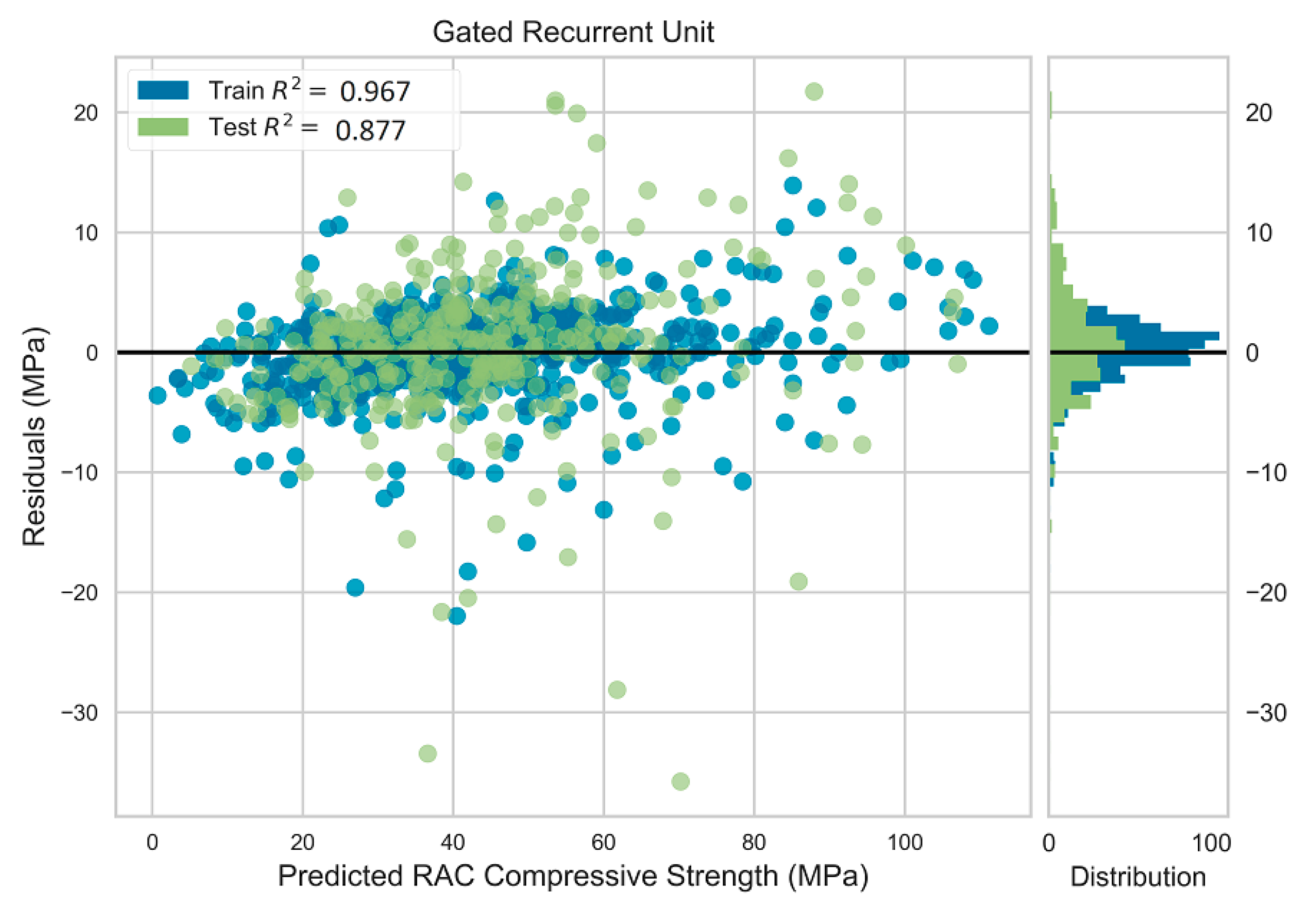
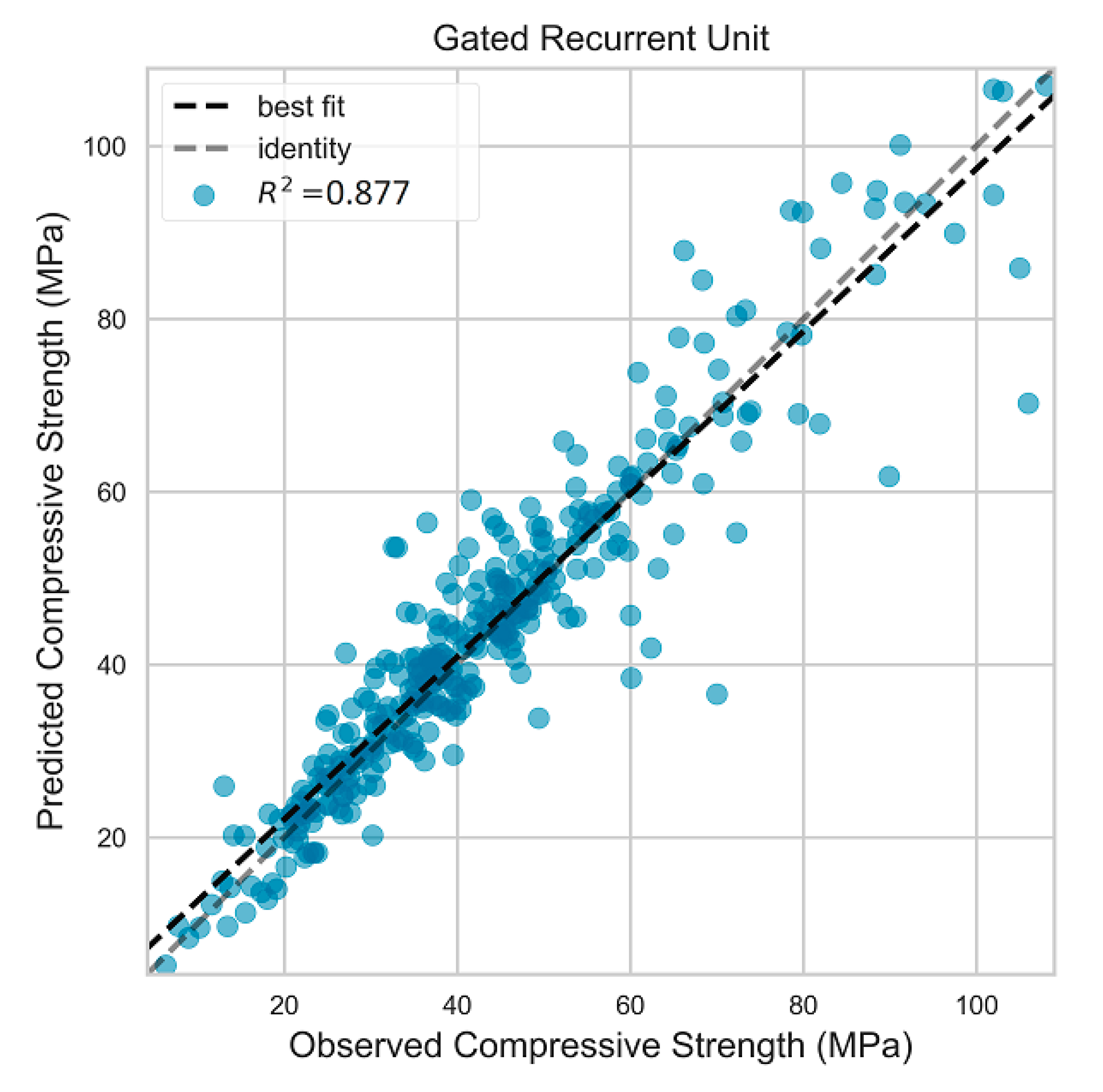
2.2. Recurrent Neural Networks
2.3. Gradient Boosting Decision Trees
3. Dataset Creation and Model Development
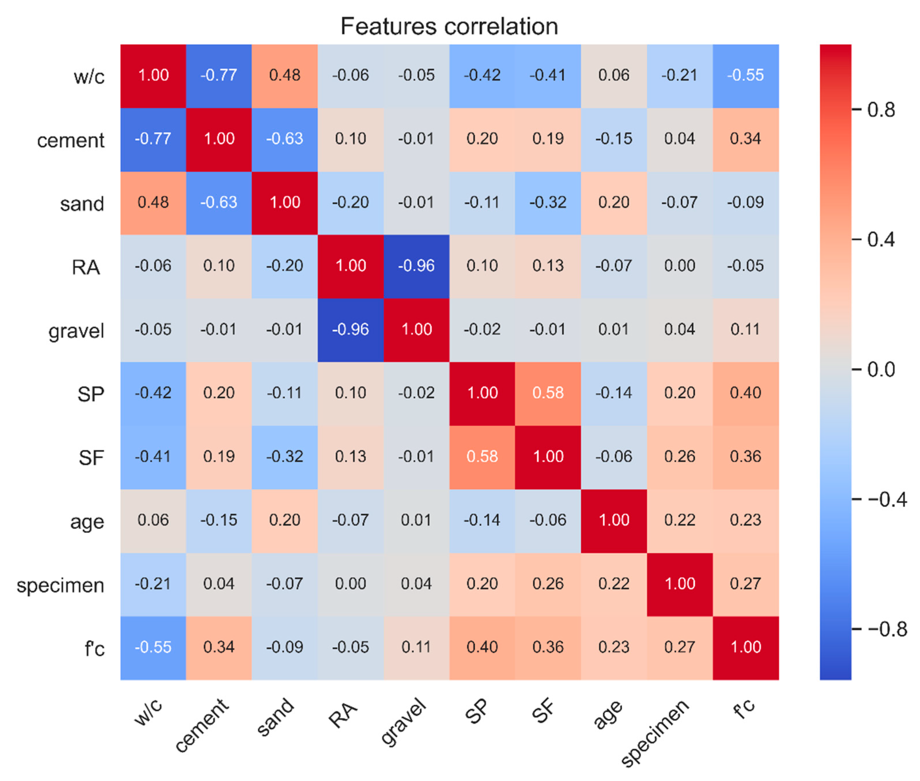
3.1. Data Collection and Preprocessing
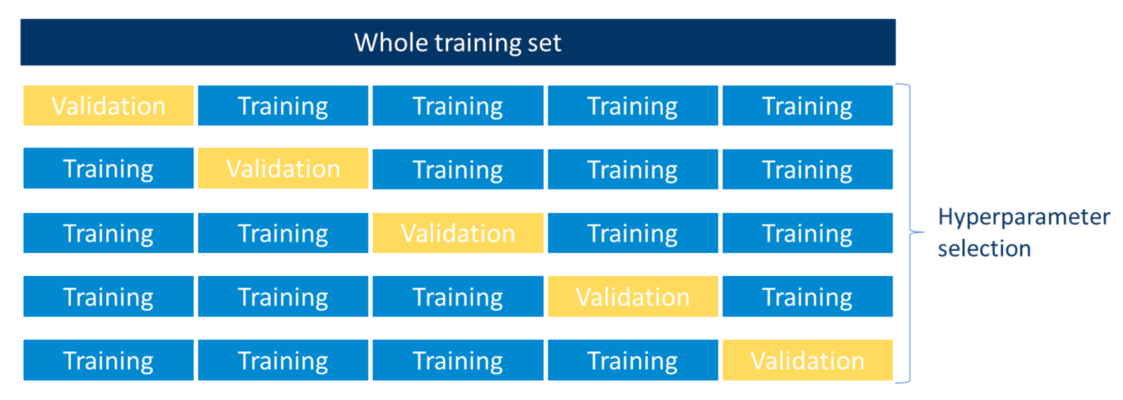
3.2. Hyperparameter Tuning
3.3. Model Development
3.3.1. GP Model
3.3.2. RNN Model
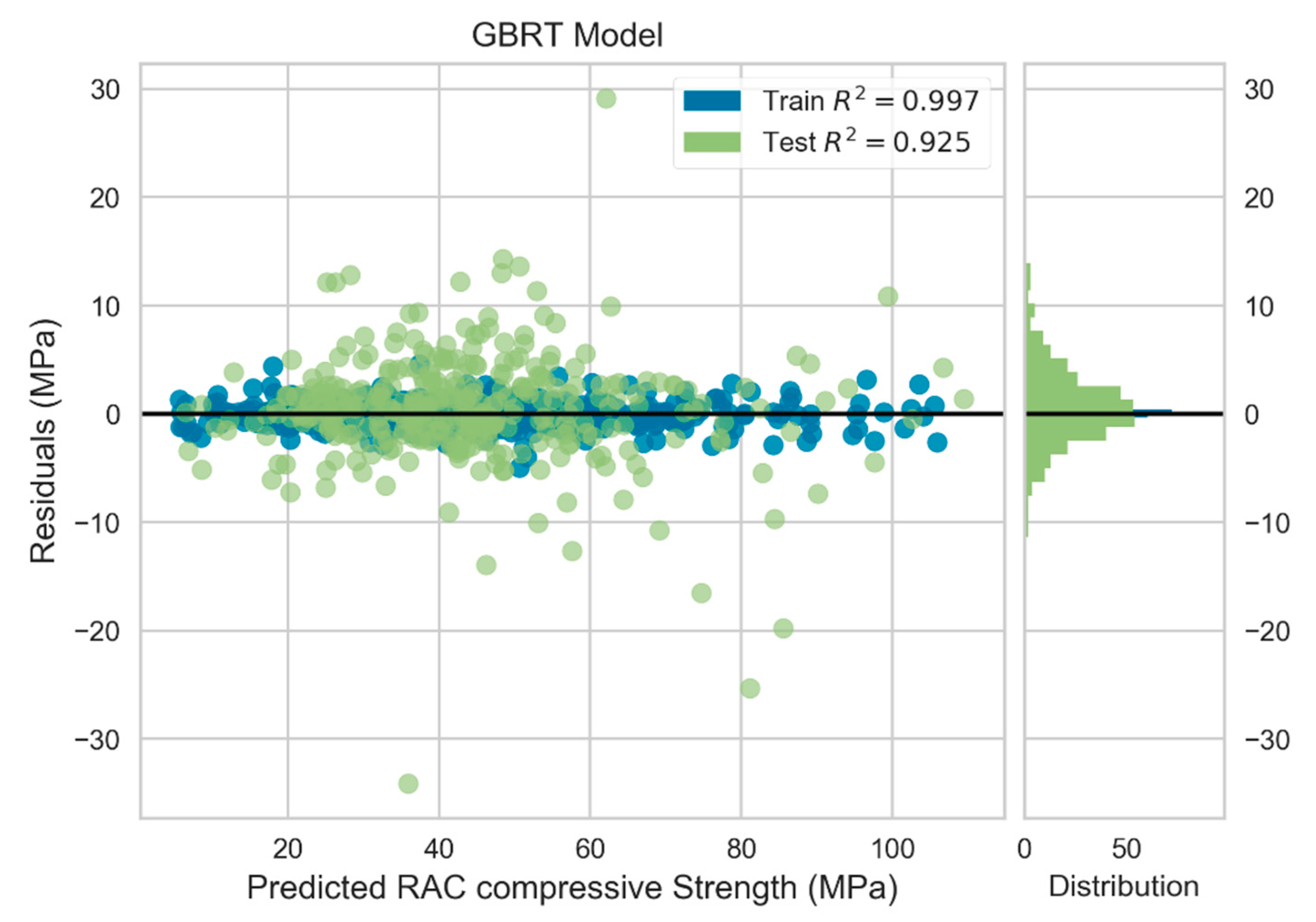
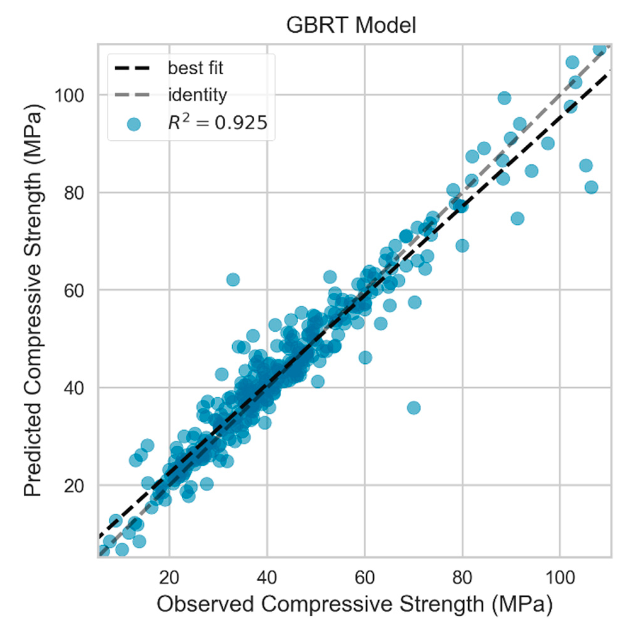
3.3.3. GBRT Model
3.4. RAC Mixture Optimization
4. Results, Discussion, and Recommendations
4.1. Prediction Performance of ML Models
4.2. Comparison of Model Performance
4.3. Comparison with Previous Studies
4.4. RAC Mixture Proportioning and Optimization
5. Conclusions
Author Contributions
Funding
Acknowledgments
Conflicts of Interest
References
- Naderpour, H.; Rafiean, A.H.; Fakharian, P. Compressive strength prediction of environmentally friendly concrete using artificial neural networks. J. Build. Eng. 2018, 16, 213–219. [Google Scholar] [CrossRef]
- Duan, Z.H.; Kou, S.C.; Poon, C.S. Prediction of compressive strength of recycled aggregate concrete using artificial neural networks. Constr. Build. Mater. 2013, 40, 1200–1206. [Google Scholar] [CrossRef]
- Gholampour, A.; Gandomi, A.H.; Ozbakkaloglu, T. New formulations for mechanical properties of recycled aggregate concrete using gene expression programming. Constr. Build. Mater. 2017, 130, 122–145. [Google Scholar] [CrossRef]
- Yeheyis, M.; Hewage, K.; Alam, M.; Eskicioglu, C.; Sadiq, R. An overview of construction and demolition waste management in Canada: A lifecycle analysis approach to sustainability. Clean Technol. Environ. Policy 2012, 15, 81–91. [Google Scholar] [CrossRef]
- Gonzalález-Fonteboa, B.; Martínez-Abella, F. Concretes with Aggregates from Demolition and Construction Waste and Silica Fume. Materials and Mechanical Properties. Build. Environ. 2008, 43, 429–437. [Google Scholar] [CrossRef]
- Topçu, I.B.; Saridemir, M.; Sarıdemir, M. Prediction of mechanical properties of recycled aggregate concretes containing silica fume using artificial neural networks and fuzzy logic. Comput. Mater. Sci. 2008, 42, 74–82. [Google Scholar] [CrossRef]
- Pedro, D.; De Brito, J.; Evangelista, L. Performance of concrete made with aggregates recycled from precasting industry waste: Influence of the crushing process. Mater. Struct. 2014, 48, 3965–3978. [Google Scholar] [CrossRef]
- Duan, Z.H.; Poon, C.S. Properties of recycled aggregate concrete made with recycled aggregates with different amounts of old adhered mortars. Mater. Des. 2014, 58, 19–29. [Google Scholar] [CrossRef]
- Poon, C.S.; Shui, Z.H.; Lam, L.; Fok, H.; Kou, S.C. Influence of moisture states of natural and recycled aggregates on the slump and compressive strength of concrete. Cem. Concr. Res. 2004, 34, 31–36. [Google Scholar] [CrossRef]
- Silva, R.V.; de Brito, J.; Dhir, R.K. The influence of the use of recycled aggregates on the compressive strength of concrete: A review. Eur. J. Environ. Civ. Eng. 2014, 19, 825–849. [Google Scholar] [CrossRef]
- Deshpande, N.; Londhe, S.; Kulkarni, S. Modeling Compressive Strength of Recycled Aggregate Concrete by Artificial Neural Network, Model Tree and Non-Linear Regression. Int. J. Sustain. Built Environ. 2014, 3, 187–198. [Google Scholar] [CrossRef] [Green Version]
- Xu, J.; Chen, Y.; Xie, T.; Zhao, X.; Xiong, B.; Chen, Z. Prediction of triaxial behavior of recycled aggregate concrete using multivariable regression and artificial neural network techniques. Constr. Build. Mater. 2019, 226, 534–554. [Google Scholar] [CrossRef]
- Xu, J.; Zhao, X.; Yu, Y.; Xie, T.; Yang, G.; Xue, J. Parametric sensitivity analysis and modelling of mechanical properties of normal- and high-strength recycled aggregate concrete using grey theory, multiple nonlinear regression and artificial neural networks. Constr. Build. Mater. 2019, 211, 479–491. [Google Scholar] [CrossRef]
- Behnood, A.; Olek, J.; Glinicki, M.A. Predicting modulus elasticity of recycled aggregate concrete using M5′ model tree algorithm. Constr. Build. Mater. 2015, 94, 137–147. [Google Scholar] [CrossRef]
- Khademi, F.; Jamal, S.M.; Deshpande, N.; Londhe, S. Predicting strength of recycled aggregate concrete using Artificial Neural Network, Adaptive Neuro-Fuzzy Inference System and Multiple Linear Regression. Int. J. Sustain. Built Environ. 2016, 5, 355–369. [Google Scholar] [CrossRef] [Green Version]
- Deng, F.; He, Y.; Zhou, S.; Yu, Y.; Cheng, H.; Wu, X. Compressive Strength Prediction of Recycled Concrete Based on Deep Learning. Constr. Build. Mater. 2018, 175, 562–569. [Google Scholar] [CrossRef]
- Ziolkowski, P.; Niedostatkiewicz, M. Machine Learning Techniques in Concrete Mix Design. Materials 2019, 12, 1256. [Google Scholar] [CrossRef] [Green Version]
- Simon, M.J. Concrete Mixture Optimization Using Statistical Methods: Final Report; Office of Infrastructure Research and Development: McLean, VA, USA, 2003.
- Yeh, I.C. Computer-Aided Design for Optimum Concrete Mixtures. Cem. Concr. Compos. 2007, 29, 193–202. [Google Scholar] [CrossRef]
- Cheng, M.-Y.; Prayogo, D.; Wu, Y.-W. Novel Genetic Algorithm-Based Evolutionary Support Vector Machine for Optimizing High-Performance Concrete Mixture. J. Comput. Civ. Eng. 2014, 28, 06014003. [Google Scholar] [CrossRef] [Green Version]
- Golafshani, E.M.; Behnood, A. Estimating the optimal mix design of silica fume concrete using biogeography-based programming. Cem. Concr. Compos. 2019, 96, 95–105. [Google Scholar] [CrossRef]
- Gholampour, A.; Mansouri, I.; Kisi, O.; Ozbakkaloglu, T. Evaluation of mechanical properties of concretes containing coarse recycled concrete aggregates using multivariate adaptive regression splines (MARS), M5 model tree (M5Tree), and least squares support vector regression (LSSVR) models. Neural Comput. Appl. 2018, 32, 295–308. [Google Scholar] [CrossRef]
- Dantas, A.T.A.; Leite, M.B.; De Jesus Nagahama, K. Prediction of compressive strength of concrete containing construction and demolition waste using artificial neural networks. Constr. Build. Mater. 2013, 38, 717–722. [Google Scholar] [CrossRef]
- Salehi, H.; Burgueño, R. Emerging artificial intelligence methods in structural engineering. Eng. Struct. 2018, 171, 170–189. [Google Scholar] [CrossRef]
- Mahdavinejad, M.S.; Rezvan, M.; Barekatain, M.; Adibi, P.; Barnaghi, P.; Sheth, A.P. Machine learning for internet of things data analysis: A survey. Digit. Commun. Netw. 2018, 4, 161–175. [Google Scholar] [CrossRef]
- Murphy, K.P. Machine Learning: A Probabilistic Perspective; MIT Press: Cambridge, MA, USA, 2012. [Google Scholar]
- Marsland, S. Machine Learning: An Algorithmic Perspective; Taylor & Francis: New York, NY, USA, 2015. [Google Scholar]
- Noori, M.; Hassani, H.; Javaherian, A.; Amindavar, H.; Torabi, S. Automatic fault detection in seismic data using Gaussian process regression. J. Appl. Geophys. 2019, 163, 117–131. [Google Scholar] [CrossRef]
- Rasmussen, C.E.; Williams, C.K.I. Gaussian Processes for Machine Learning; MIT Press: Cambridge, MA, USA, 2006. [Google Scholar]
- Omran, B.A.; Chen, Q.; Jin, R. Comparison of Data Mining Techniques for Predicting Compressive Strength of Environmentally Friendly Concrete. J. Comput. Civ. Eng. 2016, 30, 04016029. [Google Scholar] [CrossRef] [Green Version]
- Lawrence, N. Probabilistic Non-linear Principal Component Analysis with Gaussian Process Latent Variable Model. J. Mach. Learn. Res. 2005, 6, 1783–1816. [Google Scholar]
- Williams, C.K.I.; Barber, D. Bayesian classification with Gaussian processes. IEEE Trans. Pattern Anal. Mach. Intell. 1998, 20, 1342–1351. [Google Scholar] [CrossRef] [Green Version]
- Tobar, F.; Bui, T.D.; Turner, R.E. Learning stationary time series using Gaussian processes with nonparametric kernels. Adv. Neural. Inf. Process. Syst. 2015, 2015, 3501–3509. [Google Scholar]
- Lecun, Y.; Bengio, Y.; Hinton, G. Deep learning. Nature 2015, 521, 436–444. [Google Scholar] [CrossRef]
- Ye, X.W.; Jin, T.; Chen, P.Y. Structural crack detection using deep learning–based fully convolutional networks. Adv. Struct. Eng. 2019, 22, 3412–3419. [Google Scholar] [CrossRef]
- Toh, G.; Park, J. Review of vibration-based structural health monitoring using deep learning. Appl. Sci. 2020, 10, 1680. [Google Scholar] [CrossRef]
- Gulli, A.; Pal, S. Deep Learning with Keras; Packt Publishing: Birmingham, UK, 2017. [Google Scholar]
- Chollet, F. Deep Learning with Python; Manning Publigations Co.: New York, NY, USA, 2018. [Google Scholar]
- Zhao, H.; Chen, Z.; Jiang, H.; Jing, W.; Sun, L.; Feng, M. Evaluation of three deep learning models for early crop classification using Sentinel-1A imagery time series-a case study in Zhanjiang, China. Remote Sens. 2019, 11, 2673. [Google Scholar] [CrossRef] [Green Version]
- Yao, K.; Cohn, T.; Vylomova, K.; Duh, K.; Dyer, C. Depth-Gated Recurrent Neural Networks. arXiv 2015, arXiv:1508.03790. [Google Scholar]
- Zhan, X.; Zhang, S.; Szeto, W.Y.; Chen, X. Multi-step-ahead traffic speed forecasting using multi-output gradient boosting regression tree. J. Intell. Transp. Syst. Technol. Plan. Oper. 2020, 24, 125–141. [Google Scholar] [CrossRef]
- Friedman, J. Greedy Function Approximation: A Gradient Boosting Machine. Ann. Stat. 2001, 29, 1189–1232. [Google Scholar] [CrossRef]
- Persson, C.; Bacher, P.; Shiga, T.; Madsen, H. Multi-site solar power forecasting using gradient boosted regression trees. Sol. Energy 2017, 150, 423–436. [Google Scholar] [CrossRef]
- Friedman, J.H. Stochastic gradient boosting. Comput. Stat. Data Anal. 2002, 38, 367–378. [Google Scholar] [CrossRef]
- Benesty, J.; Chen, J.; Huang, Y.; Cohen, I. Noise Reduction in Speech Processing. Nat. Comput. Ser. 2009, 2, 37–40. [Google Scholar]
- Limbachiya, M.C.; Leelawat, T.; Dhir, R.K. Use of recycled concrete aggregate in high-strength concrete. Mater. Struct. Constr. 2000, 33, 574–580. [Google Scholar] [CrossRef]
- Manzi, S.; Mazzotti, C.; Bignozzi, M.C. Short and long-term behavior of structural concrete with recycled concrete aggregate. Cem. Concr. Compos. 2013, 37, 312–318. [Google Scholar] [CrossRef]
- Ajdukiewicz, A.; Kliszczewicz, A. Influence of recycled aggregates on mechanical properties of HS/HPC. Cem. Concr. Compos. 2002, 24, 269–279. [Google Scholar] [CrossRef]
- Ajdukiewicz, A.B.; Kliszczewicz, A.T. Comparative Tests of Beams and Columns Made of Recycled Aggregate Concrete and Natural Aggregate Concrete. J. Adv. Concr. Technol. 2007, 5, 259–273. [Google Scholar] [CrossRef] [Green Version]
- Gómez-Soberón, J.M.V. Porosity of recycled concrete with substitution of recycled concrete aggregate: An experimental study. Cem. Concr. Res. 2002, 32, 1301–1311. [Google Scholar] [CrossRef] [Green Version]
- Sheen, Y.-N.; Wang, H.-Y.; Juang, Y.-P.; Le, D.-H. Assessment on the engineering properties of ready-mixed concrete using recycled aggregates. Constr. Build. Mater. 2013, 45, 298–305. [Google Scholar] [CrossRef]
- Lin, Y.H.; Tyan, Y.Y.; Chang, T.P.; Chang, C.Y. An assessment of optimal mixture for concrete made with recycled concrete aggregates. Cem. Concr. Res. 2004, 34, 1373–1380. [Google Scholar] [CrossRef]
- Thomas, C.; Setién, J.; Polanco, J.A.; Alaejos, P.; de Juan, M.S. Durability of recycled aggregate concrete. Constr. Build. Mater. 2013, 40, 1054–1065. [Google Scholar] [CrossRef]
- Ulloa, V.A.; García-Taengua, E.; Pelufo, M.J.; Domingo, A.; Serna, P. New views on effect of recycled aggregates on concrete compressive strength. ACI Mater. J. 2013, 110, 687–696. [Google Scholar]
- Matias, D.; de Brito, J.; Rosa, A.; Pedro, D. Mechanical properties of concrete produced with recycled coarse aggregates—Influence of the use of superplasticizers. Constr. Build. Mater. 2013, 44, 101–109. [Google Scholar] [CrossRef]
- Taffese, W.Z. Suitability Investigation of Recycled Concrete Aggregates for Concrete Production: An Experimental Case Study. Adv. Civ. Eng. 2018, 2018, 8368351. [Google Scholar] [CrossRef]
- Etxeberria, M.; Marí, A.R.; Vázquez, E. Recycled aggregate concrete as structural material. Mater. Struct. Constr. 2007, 40, 529–541. [Google Scholar] [CrossRef]
- Andreu, G.; Miren, E. Experimental analysis of properties of high performance recycled aggregate concrete. Constr. Build. Mater. 2014, 52, 227–235. [Google Scholar] [CrossRef]
- Etxeberria, M.; Vázquez, E.; Marí, A.; Barra, M. Influence of amount of recycled coarse aggregates and production process on properties of recycled aggregate concrete. Cem. Concr. Res. 2007, 37, 735–742. [Google Scholar] [CrossRef]
- Beltrán, M.G.; Agrela, F.; Barbudo, A.; Ayuso, J.; Ramírez, A. Mechanical and durability properties of concretes manufactured with biomass bottom ash and recycled coarse aggregates. Constr. Build. Mater. 2014, 72, 231–238. [Google Scholar] [CrossRef]
- Kou, S.C.; Poon, C.S.; Chan, D. Influence of Fly Ash as Cement Replacement on the Properties of Recycled Aggregate Concrete. J. Mater. Civ. Eng. 2007, 19, 709–717. [Google Scholar] [CrossRef]
- Beltrán, M.G.; Barbudo, A.; Agrela, F.; Galvín, A.P.; Jiménez, J.R. Effect of cement addition on the properties of recycled concretes to reach control concretes strengths. J. Clean. Prod. 2014, 79, 124–133. [Google Scholar] [CrossRef]
- Poon, C.S.; Kou, S.C.; Lam, L. Influence of recycled aggregate on slump and bleeding of fresh concrete. Mater. Struct. Constr. 2007, 40, 981–988. [Google Scholar] [CrossRef]
- Çakır, Ö.; Sofyanlı, Ö.Ö. Influence of silica fume on mechanical and physical properties of recycled aggregate concrete. HBRC J. 2015, 11, 157–166. [Google Scholar] [CrossRef] [Green Version]
- Rahal, K. Mechanical properties of concrete with recycled coarse aggregate. Build. Environ. 2007, 42, 407–415. [Google Scholar] [CrossRef]
- Carneiro, J.A.; Lima, P.R.L.; Leite, M.B.; Filho, R.D.T. Compressive stress-strain behavior of steel fiber reinforced-recycled aggregate concrete. Cem. Concr. Compos. 2014, 46, 65–72. [Google Scholar] [CrossRef]
- Sato, R.; Maruyama, I.; Sogabe, T.; Sogo, M. Flexural behavior of reinforced recycled concrete beams. J. Adv. Concr. Technol. 2007, 5, 43–61. [Google Scholar] [CrossRef]
- Dilbas, H.; Şimşek, M.; Çakir, Ö. An investigation on mechanical and physical properties of recycled aggregate concrete (RAC) with and without silica fume. Constr. Build. Mater. 2014, 61, 50–59. [Google Scholar] [CrossRef]
- Casuccio, M.; Torrijos, M.C.; Giaccio, G.; Zerbino, R. Failure mechanism of recycled aggregate concrete. Constr. Build. Mater. 2008, 22, 1500–1506. [Google Scholar] [CrossRef]
- Kou, S.C.; Poon, C.S.; Chan, D. Influence of fly ash as a cement addition on the hardened properties of recycled aggregate concrete. Mater. Struct. Constr. 2008, 41, 1191–1201. [Google Scholar] [CrossRef]
- Folino, P.; Xargay, H. Recycled aggregate concrete—Mechanical behavior under uniaxial and triaxial compression. Constr. Build. Mater. 2014, 56, 21–31. [Google Scholar] [CrossRef]
- Yang, K.-H.; Chung, H.-S.; Ashou, A.F. Influence of Type and Replacement Level of Recycled Aggregates on Concrete Properties. ACI Mater. J. 2008, 105, 289–296. [Google Scholar]
- Gayarre, F.L.; Pérez, C.L.C.; López, M.A.S.; Cabo, A.D. The effect of curing conditions on the compressive strength of recycled aggregate concrete. Constr. Build. Mater. 2014, 53, 260–266. [Google Scholar] [CrossRef]
- Domingo-Cabo, A.; Lázaro, C.; López-Gayarre, F.; Serrano-López, M.A.; Serna, P.; Castaño-Tabares, J.O. Creep and shrinkage of recycled aggregate concrete. Constr. Build. Mater. 2009, 23, 2545–2553. [Google Scholar] [CrossRef]
- Medina, C.; Zhu, W.; Howind, T.; de Rojas, M.I.S.; Frías, M. Influence of mixed recycled aggregate on the physical-mechanical properties of recycled concrete. J. Clean. Prod. 2014, 68, 216–225. [Google Scholar] [CrossRef]
- Corinaldesi, V. Mechanical and elastic behaviour of concretes made of recycled-concrete coarse aggregates. Constr. Build. Mater. 2010, 24, 1616–1620. [Google Scholar] [CrossRef]
- Kumutha, R.; Vijai, K. Strength of concrete incorporating aggregates recycled from demolition waste. J. Eng. Appl. Sci. 2010, 5, 64–71. [Google Scholar]
- Pepe, M.; Filho, R.D.T.; Koenders, E.A.B.; Martinelli, E. Alternative processing procedures for recycled aggregates in structural concrete. Constr. Build. Mater. 2014, 69, 124–132. [Google Scholar] [CrossRef]
- Malešev, M.; Radonjanin, V.; Marinković, S. Recycled concrete as aggregate for structural concrete production. Sustainability 2010, 2, 1204–1225. [Google Scholar] [CrossRef] [Green Version]
- Wardeh, G.; Ghorbel, E.; Gomart, H. Mix Design and Properties of Recycled Aggregate Concretes: Applicability of Eurocode 2. Int. J. Concr. Struct. Mater. 2015, 9, 1–20. [Google Scholar] [CrossRef] [Green Version]
- Belén, G.F.; Fernando, M.A.; Diego, C.L.; Sindy, S.P. Stress-strain relationship in axial compression for concrete using recycled saturated coarse aggregate. Constr. Build. Mater. 2011, 25, 2335–2342. [Google Scholar] [CrossRef]
- Haitao, Y.; Shizhu, T. Preparation and properties of high-strength recycled concrete in cold areas. Mater. Constr. 2015, 65, 2–9. [Google Scholar] [CrossRef] [Green Version]
- Fathifazl, G.; Razaqpur, A.G.; Isgor, O.B.; Abbas, A.; Fournier, B.; Foo, S. Creep and drying shrinkage characteristics of concrete produced with coarse recycled concrete aggregate. Cem. Concr. Compos. 2011, 33, 1026–1037. [Google Scholar] [CrossRef]
- Tam, V.W.Y.; Kotrayothar, D.; Xiao, J. Long-term deformation behaviour of recycled aggregate concrete. Constr. Build. Mater. 2015, 100, 262–272. [Google Scholar] [CrossRef]
- Rao, M.C.; Bhattacharyya, S.K.; Barai, S.V. Influence of field recycled coarse aggregate on properties of concrete. Mater. Struct. Constr. 2011, 44, 205–220. [Google Scholar]
- Abdel-Hay, A.S. Properties of recycled concrete aggregate under different curing conditions. HBRC J. 2017, 13, 271–276. [Google Scholar] [CrossRef] [Green Version]
- Somna, R.; Jaturapitakkul, C.; Chalee, W.; Rattanachu, P. Effect of the Water to Binder Ratio and Ground Fly Ash on Properties of Recycled Aggregate Concrete. J. Mater. Civ. Eng. 2012, 24, 16–22. [Google Scholar] [CrossRef]
- Zheng, C.; Lou, C.; Du, G.; Li, X.; Liu, Z.; Li, L. Mechanical properties of recycled concrete with demolished waste concrete aggregate and clay brick aggregate. Results Phys. 2018, 9, 1317–1322. [Google Scholar] [CrossRef]
- Elhakam, A.A.; Mohamed, A.E.; Awad, E. Influence of self-healing, mixing method and adding silica fume on mechanical properties of recycled aggregates concrete. Constr. Build. Mater. 2012, 35, 421–427. [Google Scholar] [CrossRef]
- Nepomuceno, M.C.S.; Isidoro, R.A.S.; Catarino, J.P.G. Mechanical performance evaluation of concrete made with recycled ceramic coarse aggregates from industrial brick waste. Constr. Build. Mater. 2018, 165, 284–294. [Google Scholar] [CrossRef]
- Barbudo, A.; de Brito, J.; Evangelista, L.; Bravo, M.; Agrela, F. Influence of water-reducing admixtures on the mechanical performance of recycled concrete. J. Clean. Prod. 2013, 59, 93–98. [Google Scholar] [CrossRef]
- Mohammed, N.; Sarsam, K.; Hussien, M. The influence of recycled concrete aggregate on the properties of concrete. In MATEC Web of Conferences; EDP Sciences: Ulis, France, 2018; Volume 162, pp. 1–7. [Google Scholar]
- Butler, L.; West, J.S.; Tighe, S.L. Effect of recycled concrete coarse aggregate from multiple sources on the hardened properties of concrete with equivalent compressive strength. Constr. Build. Mater. 2013, 47, 1292–1301. [Google Scholar] [CrossRef]
- Thomas, C.; Setién, J.; Polanco, J.A.; Cimentada, A.I.; Medina, C. Influence of curing conditions on recycled aggregate concrete. Constr. Build. Mater. 2018, 172, 618–625. [Google Scholar] [CrossRef]
- Ismail, S.; Ramli, M. Engineering properties of treated recycled concrete aggregate (RCA) for structural applications. Constr. Build. Mater. 2013, 44, 464–476. [Google Scholar] [CrossRef]
- Younis, K.H.; Pilakoutas, K. Strength prediction model and methods for improving recycled aggregate concrete. Constr. Build. Mater. 2013, 49, 688–701. [Google Scholar] [CrossRef]
- Kim, K.; Shin, M.; Cha, S. Combined effects of recycled aggregate and fly ash towards concrete sustainability. Constr. Build. Mater. 2013, 48, 499–507. [Google Scholar] [CrossRef]
- Shanker, M.; Hu, M.Y.; Hung, M.S. Effect of Data Standardization on Neural Network Training. Omega Int. J. 1996, 24, 385–397. [Google Scholar] [CrossRef]
- Nilsen, V.; Pham, L.T.; Hibbard, M.; Klager, A.; Cramer, S.M.; Morgan, D. Prediction of concrete coefficient of thermal expansion and other properties using machine learning. Constr. Build. Mater. 2019, 220, 587–595. [Google Scholar] [CrossRef]
- Hastie, T.; Tibshirani, R.; Friedman, J. The Elements of Statistical Learning, 2nd ed.; Springer: Berlin/Heidelberg, Germany, 2008. [Google Scholar]
- Bardenet, R.; Brendel, M.; Kégl, B.; Sebag, M. Collaborative hyperparameter tuning. In Proceedings of the 30th International Conference on Machine Learning (ICML 2013), Atlanta, GA, USA, 16–21 June 2013; Volume 2, pp. 858–866. [Google Scholar]
- Bergstra, J.; Yamins, D.; Cox, D.D. Making a science of model search: Hyperparameter optimization in hundreds of dimensions for vision architectures. In Proceedings of the 30th International Conference on Machine Learning (ICML 2013), Atlanta, GA, USA, 16–21 June 2013; Volume 1, pp. 115–123. [Google Scholar]
- Bergstra, J.; Bengio, Y. Random search for hyper-parameter optimization. J. Mach. Learn. Res. 2012, 13, 281–305. [Google Scholar]
- Varoquaux, G.; Buitinck, L.; Louppe, G.; Grisel, O.; Pedregosa, F.; Mueller, A. Scikit-learn. GetMob. Mob. Comput. Commun. 2015, 19, 29–33. [Google Scholar] [CrossRef]
- Whang, J.; Matsukawa, A. Exploring Batch Normalization in Recurrent Neural Networks. Stanford Center for Professional Development. Available online: https://jaywhang.com/assets/batchnorm_rnn.pdf (accessed on 28 September 2020).
- Ioffe, S.; Szegedy, C. Batch normalization: Accelerating deep network training by reducing internal covariate shift. In Proceedings of the 32nd International Conference on Machine Learning (ICML 2015), Lille, France, 6–11 July 2015; Volume 1, pp. 448–456. [Google Scholar]
- Chollet, F. Keras. GitHub Repository. 2015. Available online: https://github.com/fchollet/keras (accessed on 28 September 2020).
- Marani, A.; Nehdi, M.L. Machine learning prediction of compressive strength for phase change materials integrated cementitious composites. Constr. Build. Mater. 2020, 265, 120286. [Google Scholar] [CrossRef]
- Penadés-Plà, V.; García-Segura, T.; Martí, J.V.; Yepes, V. A review of multi-criteria decision-making methods applied to the sustainable bridge design. Sustainability 2016, 8, 1295. [Google Scholar] [CrossRef] [Green Version]
- Lu, P.; Chen, S.; Zheng, Y. Artificial intelligence in civil engineering. Math. Probl. Eng. 2012, 2012, 1–22. [Google Scholar] [CrossRef] [Green Version]
- Wijayasundara, M.; Mendis, P.; Zhang, L.; Sofi, M. Financial assessment of manufacturing recycled aggregate concrete in ready-mix concrete plants. Resour. Conserv. Recycl. 2016, 109, 187–201. [Google Scholar] [CrossRef]


| Machine Learning Technique | No. of Samples | Ref. |
|---|---|---|
| Artificial neural networks, adaptive neuro-fuzzy inference system and multiple linear regression | 257 | [15] |
| Artificial neural networks | 168 | [2] |
| Artificial neural networks, model tree and non-linear regression model | 257 | [11] |
| Artificial neural networks and fuzzy logic | 210 | [6] |
| Convolutional neural networks | 74 | [16] |
| Artificial neural networks | 139 | [1] |
| Artificial neural networks | 1178 | [23] |
| Multivariate adaptive regression splines, M5 model tree and least support vector regression | 650 | [22] |
| Authors | No. of Samples | Ref. | Authors | No. of Samples | Ref. |
|---|---|---|---|---|---|
| M. C. Limbachiya et al. | 12 | [46] | S. Manzi et al. | 10 | [47] |
| A. Ajdukiewicz and A. Kliszczewicz | 117 | [48] | A. B. Ajdukiewicz & A. T. Kliszczewicz | 16 | [49] |
| J. M. V. Gómez-Soberón | 15 | [50] | Y.-N. Sheen et al. | 27 | [51] |
| Y. H. Lin et al. | 24 | [52] | C. Thomas et al. | 72 | [53] |
| C. S. Poon et al. | 36 | [9] | V. A. Ulloa et al. | 18 | [54] |
| D. Matias et al. | 9 | [55] | W. Z. Taffese | 10 | [56] |
| M. Etxeberria et al. | 4 | [57] | G. Andreu and E. Miren | 30 | [58] |
| M. Etxeberria et al. | 12 | [59] | M. G. Beltrán et al. | 9 | [60] |
| S. C. Kou et al. | 40 | [61] | M. G. Beltrán et al. | 8 | [62] |
| C. S. Poon et al. | 8 | [63] | Ö. Çakır and Ö. Ö. Sofyanlı | 27 | [64] |
| K. Rahal | 70 | [65] | J. A. Carneiro et al. | 2 | [66] |
| R. Sato et al. | 11 | [67] | H. Dilbas et al. | 12 | [68] |
| M. Casuccio et al. | 9 | [69] | Z. H. Duan and C. S. Poon | 26 | [8] |
| S. C. Kou et al. | 24 | [70] | P. Folino and H. Xargay | 4 | [71] |
| K.-H. Yang et al. | 42 | [72] | F. López Gayarre et al. | 14 | [73] |
| A. Domingo-Cabo et al. | 8 | [74] | C. Medina et al. | 16 | [75] |
| V. Corinaldesi | 10 | [76] | D. Pedro et al. | 18 | [7] |
| R. Kumutha and K. Vijai | 12 | [77] | M. Pepe et al. | 15 | [78] |
| M. Malešev et al. | 9 | [79] | G. Wardeh et al. | 16 | [80] |
| G. F. Belén et al. | 16 | [81] | Y. Haitao and T. Shizhu | 20 | [82] |
| G. Fathifazl et al. | 6 | [83] | V. W. Y. Tam et al. | 24 | [84] |
| M. Chakradhara Rao et al. | 16 | [85] | A. S. Abdel-Hay | 4 | [86] |
| R. Somna | 18 | [87] | C. Zheng et al. | 36 | [88] |
| A. Abd Elhakam et al. | 30 | [89] | M. C. S. Nepomuceno et al. | 15 | [90] |
| A. Barbudo et al. | 36 | [91] | N. Mohammed et al. | 12 | [92] |
| L. Butler et al. | 8 | [93] | C. Thomas et al. | 23 | [94] |
| S. Ismail and M. Ramli | 12 | [95] | K. H. Younis and K. Pilakoutas | 18 | [96] |
| K. Kim et al. | 18 | [97] |
| Input Feature | Units | Min. | Max. | Mean | Standard Deviation |
| Water-to-cement ratio | - | 0.24 | 1.02 | 0.49 | 0.12 |
| Cement content | kg/m3 | 210.00 | 650.00 | 387.60 | 71.36 |
| Sand content | kg/m3 | 419.52 | 1010.00 | 691.71 | 131.65 |
| Recycled aggregate content | kg/m3 | 0.00 | 1358.00 | 527.83 | 444.75 |
| Gavel content | kg/m3 | 0.00 | 1524.00 | 542.94 | 470.19 |
| Superplasticizer | kg/m3 | 0.00 | 45.00 | 2.63 | 4.53 |
| Silica fume content | kg/m3 | 0.00 | 50.00 | 3.47 | 11.60 |
| Age | Days | 2.00 | 365.00 | 44.57 | 70.69 |
| Specimen type | Type | 1.00 | 5.00 | 2.79 | 1.15 |
| Output | Units | Min. | Max. | Mean | Standard Deviation |
| Compressive strength | MPa | 4.30 | 108.51 | 43.57 | 17.72 |
| Hyperparameter | Assigned Value |
|---|---|
| Length scale 1, | 0.6 |
| Periodicity, | 16.0 |
| Sigma naught, | 1.9 |
| Length scale 2, | 1 |
| Nu, | 0.5 |
| Layer | Units | Activation Function | Recurrent Activation Function | Kernel Initializer | Recurrent Initializer |
|---|---|---|---|---|---|
| Gated recurrent unit | 239 | ReLU | Sigmoid | Random Uniform | Constant |
| Gated recurrent unit | 238 | Sigmoid | ReLU | Random Uniform | Zeros |
| Gated recurrent unit | 217 | SELU | Softsign | Constant | Zeros |
| Dense | 1 | Softplus | - | - | - |
| Hyperparameter | Number of Estimators | Learning Rate | Min Samples Split | Min Samples Leaf | Max Depth | Max Features | Subsample |
|---|---|---|---|---|---|---|---|
| Value | 315 | 0.44 | 33 | 17 | 5 | 7 | 0.98 |
| Ingredient | Units | Currency | Unit Price |
|---|---|---|---|
| Water | $/kg | Canadian dollar | 0.004 |
| Cement | $/kg | Canadian dollar | 0.43 |
| Sand | $/kg | Canadian dollar | 0.28 |
| Recycled coarse aggregate | $/kg | Canadian dollar | 0.20 |
| Gavel | $/kg | Canadian dollar | 0.20 |
| Superplasticizer | $/kg | Canadian dollar | 71.07 |
| Silica fume | $/kg | Canadian dollar | 2.85 |
| Input Feature | Unit | 25 MPa | 30 MPa | 35 MPa | 40 MPa | ||||
|---|---|---|---|---|---|---|---|---|---|
| Upper Limit | Lower Limit | Upper Limit | Lower Limit | Upper Limit | Lower Limit | Upper Limit | Lower Limit | ||
| Water | kg/m3 | 350 | 200 | 350 | 190 | 230 | 160 | 230 | 160 |
| Cement | kg/m3 | 424 | 290 | 424 | 292 | 424 | 323 | 424 | 280 |
| Sand | kg/m3 | 942 | 650 | 942 | 650 | 942 | 720 | 942 | 750 |
| RCA a | kg/m3 | 1080 | 700 | 1080 | 750 | 1080 | 550 | 900 | 750 |
| Gavel | kg/m3 | 511 | 50 | 511 | 50 | 511 | 100 | 750 | 220 |
| SP b | kg/m3 | 0 | 0 | 0 | 0 | 0 | 0 | 2 | 0.9 |
| Age | Days | 28 | 28 | 28 | 28 | 28 | 28 | 28 | 28 |
| Specimen | Type | 1 | 1 | 1 | 1 | 1 | 1 | 1 | 1 |
| Optimized Mix | Water | Cement | Sand | RCA a | Gravel | SP b | Age | ST c |
|---|---|---|---|---|---|---|---|---|
| (kg/m3) | (kg/m3) | (kg/m3) | (kg/m3) | (kg/m3) | (kg/m3) | Days | Type | |
| 25 MPa | 246.46 | 296.62 | 701.67 | 711.90 | 155.23 | 0.00 | 28 | 1 |
| 30 MPa | 239.56 | 298.52 | 701.67 | 760.33 | 155.23 | 0.00 | 28 | 1 |
| 35 MPa | 181.68 | 327.99 | 759.29 | 566.60 | 193.82 | 0.00 | 28 | 1 |
| 40 MPa | 178.83 | 310.45 | 767.23 | 768.92 | 313.78 | 1.23 | 28 | 1 |
| Input Feature | Units | 25 MPa | 30 MPa | 35 MPa | 40 MPa | ||||
|---|---|---|---|---|---|---|---|---|---|
| Base | Opt. | Base | Opt. | Base | Opt. | Base | Opt. | ||
| Water | kg/m3 | 234.10 | 246.46 | 190.00 | 239.56 | 175.00 | 181.68 | 187.00 | 178.83 |
| Cement | kg/m3 | 390.16 | 296.62 | 380.00 | 298.52 | 350.00 | 327.99 | 311.00 | 310.45 |
| Sand | kg/m3 | 702.30 | 701.67 | 637.00 | 701.67 | 730.00 | 759.29 | 840.00 | 767.23 |
| RCA a | kg/m3 | 1053.45 | 711.90 | 1123.00 | 760.33 | 989.00 | 566.60 | 0.00 | 768.92 |
| Gravel | kg/m3 | 0.00 | 155.23 | 0.00 | 155.23 | 0.00 | 193.82 | 935.00 | 313.78 |
| SP b | kg/m3 | 0.00 | 0.00 | 0.00 | 0.00 | 1.68 | 0.00 | 1.56 | 1.23 |
| Age | Days | 28 | 28 | 28 | 28 | 28 | 28 | 28 | 28 |
| ST c | Type | 1 | 1 | 1 | 1 | 1 | 1 | 1 | 1 |
| F’c | MPa | 25.3 | 25.5 | 30.1 | 29.6 | 36.0 | 35.5 | 40.0 | 39.9 |
| Price | CAD | 577.21 | 499.44 | 568.49 | 510.02 | 673.94 | 507.12 | 668.66 | 654.35 |
| Random Seed and Global Performance | Set | RMSE b | MAE c | R2 |
|---|---|---|---|---|
| RS a = 59 | Test | 7.468 | 5.157 | 0.827 |
| Train | 0.556 | 0.111 | 0.999 | |
| RS a = 1718 | Test | 7.589 | 5.197 | 0.834 |
| Train | 0.789 | 0.144 | 0.998 | |
| RS a = 1009 | Test | 6.582 | 4.762 | 0.854 |
| Train | 0.595 | 0.103 | 0.999 | |
| RS a = 3097 | Test | 7.492 | 4.875 | 0.841 |
| Train | 0.680 | 0.135 | 0.998 | |
| RS a = 7 | Test | 6.305 | 4.566 | 0.862 |
| Train | 1.055 | 0.197 | 0.997 | |
| Average | Test | 7.087 | 4.911 | 0.844 |
| Train | 0.735 | 0.138 | 0.998 | |
| Standard Deviation | Test | 0.597 | 0.267 | 0.014 |
| Train | 0.200 | 0.037 | 0.001 |
| Random Seed and Global Performance | Set | RMSE b | MAE c | R2 |
|---|---|---|---|---|
| RS a = 59 | Test | 7.298 | 4.663 | 0.835 |
| Train | 3.064 | 2.16 | 0.97 | |
| RS a = 1718 | Test | 6.927 | 4.567 | 0.861 |
| Train | 3.140 | 2.274 | 0.968 | |
| RS a = 1009 | Test | 5.778 | 4.106 | 0.888 |
| Train | 3.172 | 2.316 | 0.969 | |
| RS a = 3097 | Test | 6.589 | 4.312 | 0.877 |
| Train | 3.144 | 2.251 | 0.967 | |
| RS a = 7 | Test | 5.918 | 4.172 | 0.878 |
| Train | 3.394 | 2.422 | 0.965 | |
| Average | Test | 6.502 | 4.364 | 0.868 |
| Train | 3.183 | 2.285 | 0.968 | |
| Standard Deviation | Test | 0.649 | 0.243 | 0.021 |
| Train | 0.125 | 0.096 | 0.002 |
| Random Seed and Global Performance | Set | RMSE b | MAE c | R2 |
|---|---|---|---|---|
| RS a = 59 | Test | 5.124 | 3.354 | 0.918 |
| Train | 1.102 | 0.743 | 0.996 | |
| RS a = 1718 | Test | 5.359 | 3.698 | 0.917 |
| Train | 1.008 | 0.710 | 0.996 | |
| RS a = 1009 | Test | 4.640 | 3.196 | 0.927 |
| Train | 0.965 | 0.683 | 0.997 | |
| RS a = 3097 | Test | 5.168 | 3.335 | 0.924 |
| Train | 0.970 | 0.704 | 0.996 | |
| RS a = 7 | Test | 5.087 | 3.398 | 0.911 |
| Train | 1.052 | 0.748 | 0.996 | |
| Mean | Test | 5.076 | 3.396 | 0.919 |
| Train | 1.019 | 0.718 | 0.996 | |
| Standard Deviation | Test | 0.236 | 0.165 | 0.005 |
| Train | 0.051 | 0.024 | 0.0003 |
| Machine Learning Technique | R2 | RMSE | No. of Samples | Ref. |
|---|---|---|---|---|
| Multiple linear regression | 0.609 | 9.975 | 257 | [15] |
| Artificial neural networks | 0.919 | 4.446 | ||
| Adaptive neuro-fuzzy inference system | 0.908 | 5.045 | ||
| Artificial neural networks | 0.995 | 3.6804 | 168 | [2] |
| Artificial neural networks | 0.903 | - | 257 | [11] |
| Model tree | 0.757 | - | ||
| Non-linear regression model | 0.740 | - | ||
| Artificial neural networks | 0.998 | 2.395 | 210 | [6] |
| Fuzzy logic | 0.996 | 3.866 | ||
| Artificial neural networks | 0.688 | - | 139 | [1] |
| Artificial neural networks | 0.971 | - | 1178 | [23] |
| Multivariate adaptive regression splines | - | 8.750 | 650 | [22] |
| M5 model tree | - | 8.250 | ||
| Least support vector regression | - | 7.550 | ||
| Gradient Boosting a | 0.919 | 5.076 | 1134 | - |
| Deep Learning a | 0.868 | 6.502 |
© 2020 by the authors. Licensee MDPI, Basel, Switzerland. This article is an open access article distributed under the terms and conditions of the Creative Commons Attribution (CC BY) license (http://creativecommons.org/licenses/by/4.0/).
Share and Cite
Nunez, I.; Marani, A.; Nehdi, M.L. Mixture Optimization of Recycled Aggregate Concrete Using Hybrid Machine Learning Model. Materials 2020, 13, 4331. https://doi.org/10.3390/ma13194331
Nunez I, Marani A, Nehdi ML. Mixture Optimization of Recycled Aggregate Concrete Using Hybrid Machine Learning Model. Materials. 2020; 13(19):4331. https://doi.org/10.3390/ma13194331
Chicago/Turabian StyleNunez, Itzel, Afshin Marani, and Moncef L. Nehdi. 2020. "Mixture Optimization of Recycled Aggregate Concrete Using Hybrid Machine Learning Model" Materials 13, no. 19: 4331. https://doi.org/10.3390/ma13194331