Simulation of Shape Memory Alloy (SMA)-Bias Spring Actuation for Self-Shaping Architecture: Investigation of Parametric Sensitivity


Abstract
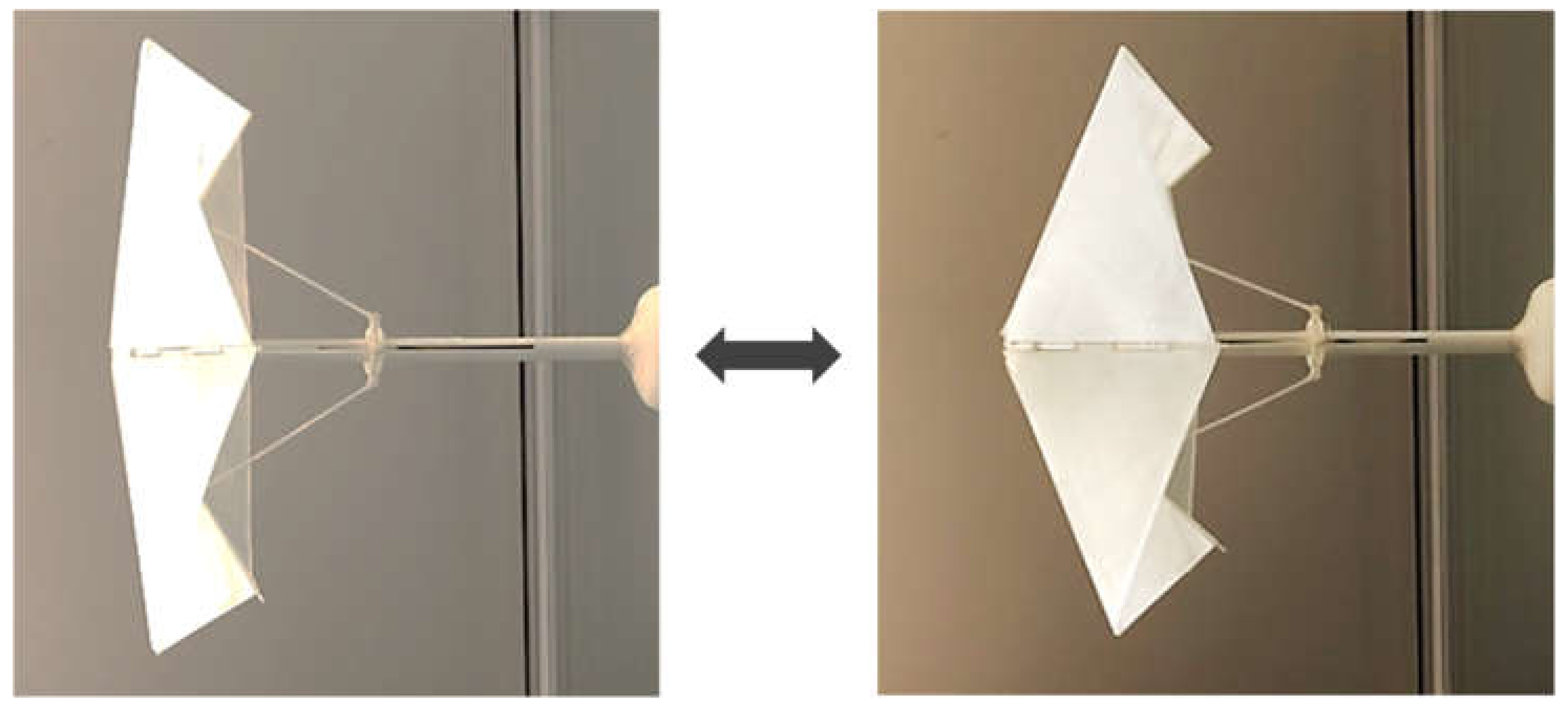
:1. Introduction
2. Materials and Methods
2.1. Theoretical SMA Constitutive Model
2.2. Modeling of 1-D SMA-Bias Spring Actuation
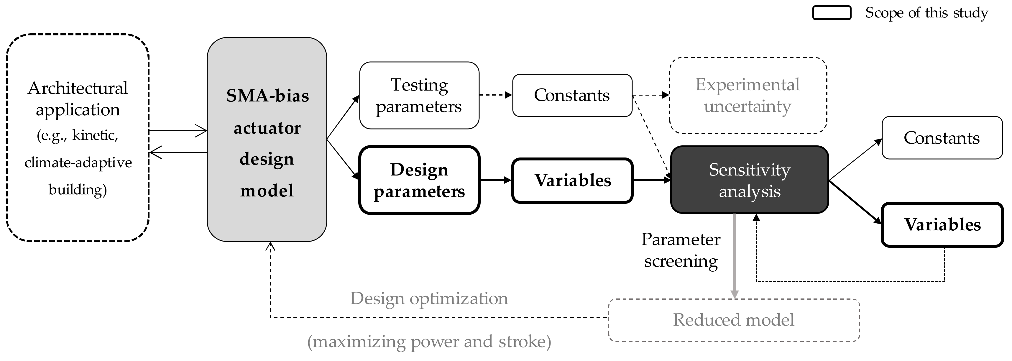
2.3. Sensitivity Analysis (SA) and Monte Carlo Approach to Simulation
2.4. Study Parameters
3. Results and Discussion
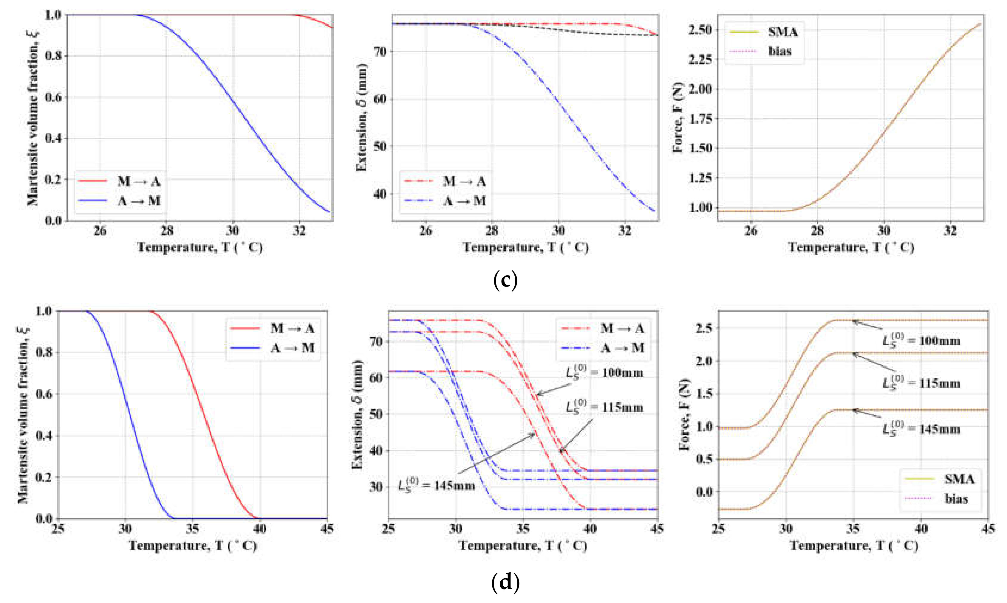
3.1. Experimental Parameter Investigation
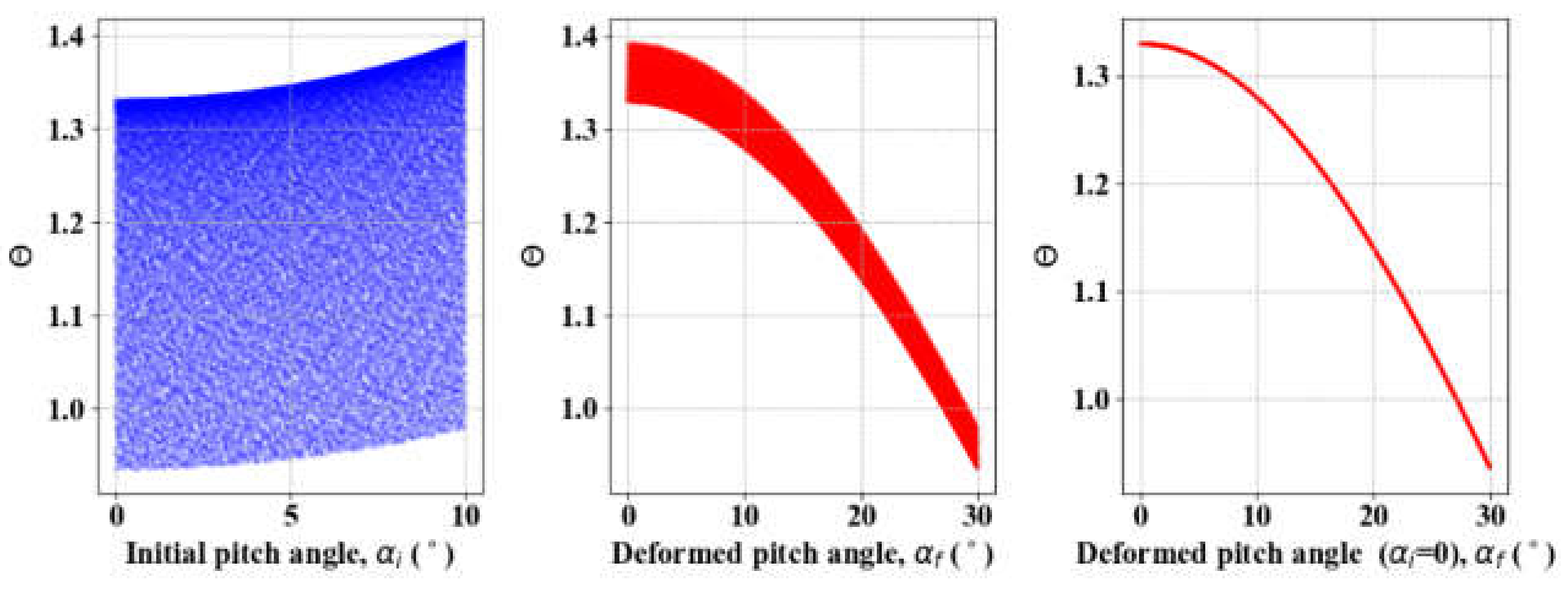
3.2. SA: Spring Pitch Angle Variation
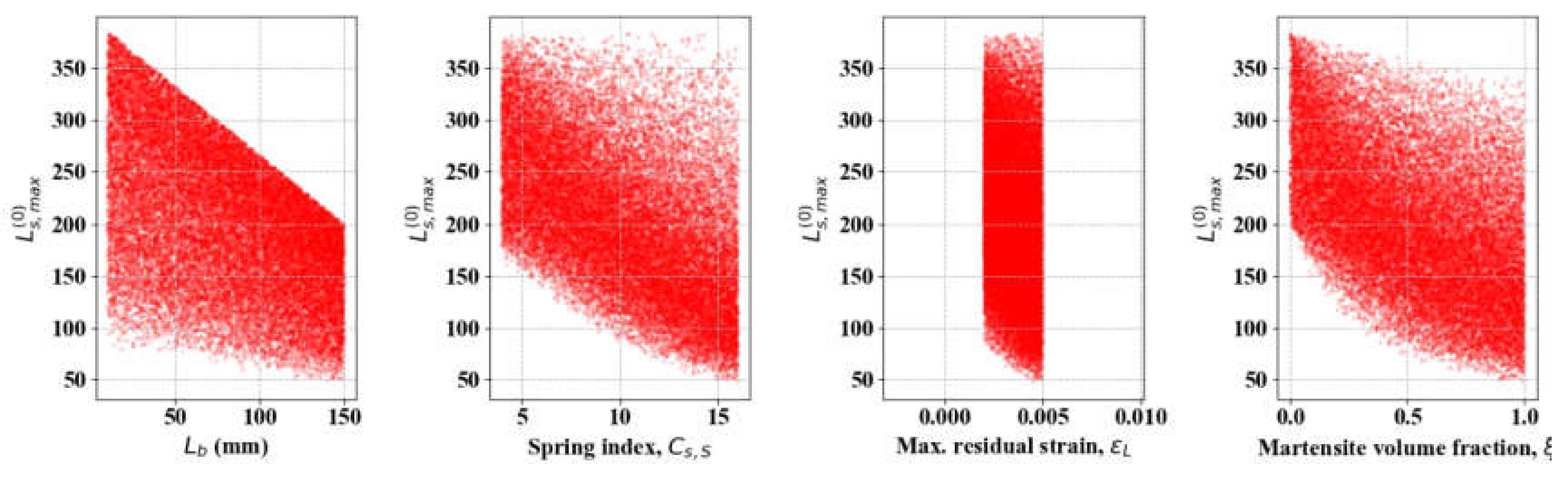
3.3. SA: Limit of Initial SMA Length ()
3.4. SA: SMA Displacement ()
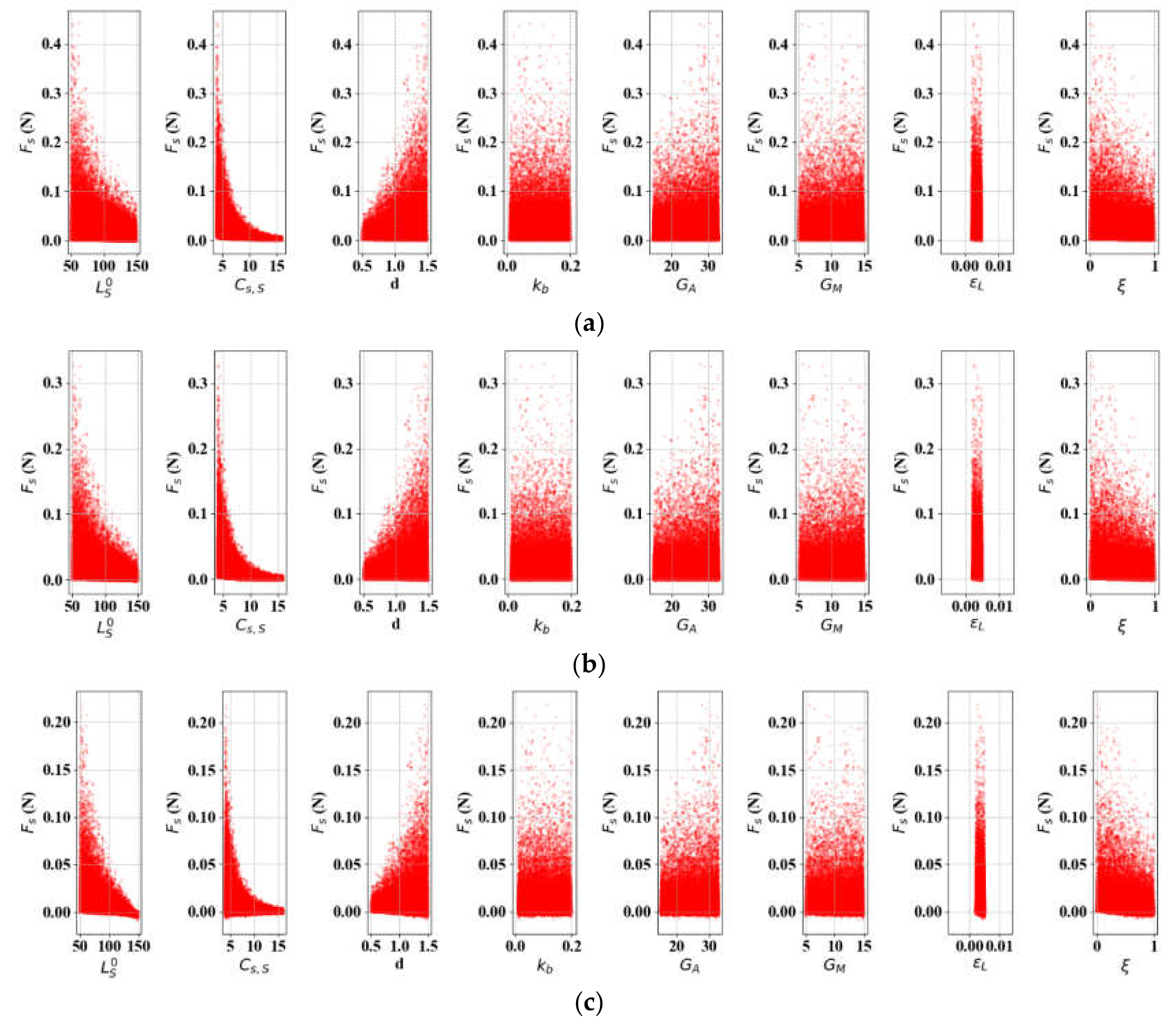
3.5. SA: Actuation Force ()
3.6. SA: Maximum Output Stroke and Force
4. Discussion and Concluding Remarks
4.1. Rankings of Parameter Importance in SMA-Bias Actuator Design
4.2. Trade-Off between Output Stroke and Force
4.3. Temperature Dependency of Actuator Performance
4.4. Reduction in Model Complexity and Uncertainty in SA
Funding
Acknowledgments
Conflicts of Interest
Nomenclature
| Abbreviation | ||
| Specific Helmholtz free energy | J/g | |
| A, M | Austenite, martensite | - |
| , | Austenitic (A) and martensitic (M) alloy stiffness | N/mm2 |
| Martensite volume fraction | - | |
| , | Stress-temperature curve gradient in austenite and martensite | - |
| Specific enthalpy (latent heat) | J/g | |
| Coefficient of spring pitch angles | - | |
| L | Total length of actuator spring connection | mm |
| Original length of bias spring | mm | |
| Original length of shape memory alloy (SMA) spring | mm | |
| SMA spring shear modulus | N/mm2 | |
| SMA spring deflection | mm | |
| Output stroke of actuation | mm | |
| SMA spring force | N | |
| Output force of actuation | N | |
| SMA spring index | - | |
| Bias spring coefficient | N/mm | |
| Residual strain | - | |
| ST | Total Sobol index | - |
| Critical temperature | °C |
References
- Elahinia, M.H. Shape Memory Alloy Actuators: Design, Fabrication, and Experimental Evaluation; John Wiley & Sons, Ltd.: West Sussex, UK, 2016. [Google Scholar]
- Rogers, C.A.; Giurgiutiu, V.; Leung, C.K.Y. Smart Materials for Civil Engineering Application. In Emerging Materials for Civil Infrastructure: State of the Art; Lopez-Anido, R.A., Naik, T.R., Eds.; American Society of Civil Engineers (ASCE): Reston, VA, USA, 2000. [Google Scholar]
- Lecce, L.; Concilio, A. Shape Memory Alloy Engineering for Aerospace, Structural and Biomedical Applications; Butterworth-Heinemann: Oxford, UK, 2014. [Google Scholar]
- Jani, J.M.; Leary, M.; Subic, A.; Gibson, M.A. A review of shape memory alloy research, applications and opportunities. Mater. Des. 2014, 56, 1078–1113. [Google Scholar] [CrossRef]
- Arun, D.I.; Chakravarthy, P.; Arockia Kumar, R.; Santhosh, B. Shape Memory Materials, 1st ed.; CRC Press: Boca Raton, FL, USA, 2018. [Google Scholar]
- Sellitto, A.; Riccio, A. Overview and Future Advanced Engineering Applications for Morphing Surfaces by Shape Memory Alloy Materials. Materials 2019, 12, 708. [Google Scholar] [CrossRef] [PubMed] [Green Version]
- Grinham, J.; Blabolil, R.; Haak, J. Harvest Shade Screens: Programming Material for Optimal Energy Building Skins. In Proceedings of the 34th Annual Conference of the Association for Computer Aided Design in Architecture (ACADIA), Los Angeles, CA, USA, 23 October 2014; pp. 281–290. [Google Scholar]
- Formentini, M.; Lenci, S. An innovative building envelope (kinetic façade) with Shape Memory Alloys used as actuators and sensors. Autom. Constr. 2018, 85, 220–231. [Google Scholar] [CrossRef]
- Vazquez, E.; Randall, C.; Duarte, J.P. Shape-changing Architectural Skins: A Review on Materials, Design and Fabrication Strategies and Performance Analysis. J. Facade Des. Eng. 2019, 7, 93–114. [Google Scholar]
- Yi, H.; Kim, D.; Kim, Y.; Kim, D.; Koh, J.-S.; Kim, M.-J. 3d-Printed Attachable Kinetic Shading Device with Alternate Actuation: Use of Shape-Memory Alloy (SMA) for Climate-Adaptive Responsive Architecture. Autom. Constr. 2020, 114, 103151. [Google Scholar] [CrossRef]
- Andani, M.T.; Bucchi, F.; Elahinia, M.H. Sma Actuation Mechanisms. In Shape Memory Alloy Actuators: Design, Fabrication, and Experimental Evaluation; Elahinia, M.H., Ed.; John Wiley & Sons, Ltd.: West Sussex, UK, 2016; pp. 85–123. [Google Scholar]
- White, E.L.; Case, J.C.; Kramer-Bottiglio, R. A Soft Parallel Kinematic Mechanism. Soft Robot. 2018, 5, 36–53. [Google Scholar] [CrossRef]
- Boufayed, R.; Chapelle, F.; Destrebecq, J.F.; Balandraud, X. Finite element analysis of a prestressed mechanism with multi-antagonistic and hysteretic SMA actuation. Meccanica 2020, 55, 1–18. [Google Scholar] [CrossRef]
- Degeratu, S.; Bizdoaca, N.G.; Manolea, G.; Diaconu, I.; Petrisor, A.; Degeratu, V. On the Design of a Shape Memory Alloy Spring Actuator Using Thermal Analysis. WSEAS Trans. Syst. 2008, 7, 1006–1015. [Google Scholar]
- Tanaka, K.A. Thermomechanical Sketch of Shape Memory Effect: One-Dimensional Tensile Behavior. Res. Mech. 1986, 18, 251–263. [Google Scholar]
- Brinson, L. One-Dimensional Constitutive Behavior of Shape Memory Alloys: Thermomechanical Derivation with Non-Constant Material Functions and Redefined Martensite Internal Variable. J. Intell. Mater. Syst. Struct. 1993, 4, 229–242. [Google Scholar] [CrossRef]
- Liang, C.; Rogers, C.A. One-Dimensional Thermomechanical Constitutive Relations for Shape Memory Materials. J. Intell. Mater. Syst. Struct. 1997, 8, 285–302. [Google Scholar] [CrossRef]
- An, S.-M.; Ryu, J.; Cho, M.; Cho, K.-J. Engineering design framework for a shape memory alloy coil spring actuator using a static two-state model. Smart Mater. Struct. 2012, 21, 55009. [Google Scholar] [CrossRef]
- Fortini, A.; Merlin, M.; Rizzoni, R.; Marfia, S. TWSME of a NiTi strip in free bending conditions: Experimental and theoretical approach. Frattura Integr. Strutt. 2014, 8, 74–84. [Google Scholar] [CrossRef] [Green Version]
- Spaggiari, A.; Spinella, I.; Dragoni, E. Design equations for binary shape memory actuators under arbitrary external forces. J. Intell. Mater. Syst. Struct. 2012, 24, 682–694. [Google Scholar] [CrossRef]
- Yoo, Y.-I.; Kim, Y.-J.; Shin, D.-K.; Lee, J.-J. Development of martensite transformation kinetics of NiTi shape memory alloys under compression. Int. J. Solids Struct. 2015, 64, 51–61. [Google Scholar] [CrossRef]
- Xia, L.; Yang, M.; Li, L.; Zhang, X. Aerodynamic Design Based on Global Sensitivity Analysis Method. Xibei Gongye Daxue Xuebao/J. Northwest. Polytech. Univ. 2018, 36, 49–56. [Google Scholar] [CrossRef] [Green Version]
- Gan, Y.; Duan, Q.; Gong, W.; Tong, C.; Sun, Y.; Chu, W.; Ye, A.; Miao, C.; Di, Z. A comprehensive evaluation of various sensitivity analysis methods: A case study with a hydrological model. Environ. Model. Softw. 2014, 51, 269–285. [Google Scholar] [CrossRef] [Green Version]
- Shirani, M.; Kadkhodaei, M. One dimensional constitutive model with transformation surfaces for phase transition in shape memory alloys considering the effect of loading history. Int. J. Solids Struct. 2016, 81, 117–129. [Google Scholar] [CrossRef]
- Associated Spring RAYMOND. Design Handbook: Engineering Guide to Spring Design; Barnes Group Inc.: Bristol, CT, USA, 1988. [Google Scholar]
- Duerig, T.W.; Bhattacharya, K. The Influence of the R-Phase on the Superelastic Behavior of NiTi. Shape Mem. Superelasticity 2015, 1, 153–161. [Google Scholar] [CrossRef]
- Zhang, X.; Sehitoglu, H. Crystallography of the B2→R→B19′ phase transformations in NiTi. Mater. Sci. Eng. A 2004, 374, 292–302. [Google Scholar] [CrossRef]
- Koh, J.-S. Design of Shape Memory Alloy Coil Spring Actuator for Improving Performance in Cyclic Actuation. Materials 2018, 11, 2324. [Google Scholar] [CrossRef] [PubMed] [Green Version]
- Islam, A.B.M.R.; Karadoğan, E. Analysis of One-Dimensional Ivshin–Pence Shape Memory Alloy Constitutive Model for Sensitivity and Uncertainty. Materials 2020, 13, 1482. [Google Scholar] [CrossRef] [PubMed] [Green Version]


| Model Output | Design Parameter (■) | Testing Parameter (□) | ||||||||||||||
|---|---|---|---|---|---|---|---|---|---|---|---|---|---|---|---|---|
| 1 | ■ | ■ | ||||||||||||||
| 1 | ■ | ■ | ■ | ■ | ■ | □ | □ | □ | □ | □ | □ | |||||
| 1 | ■ | ■ | ■ | ■ | ■ | ■ | ■ | ■ | □ | □ | □ | □ | □ | □ | □ | □ |
| ■ | ■ | ■ | ■ | ■ | ■ | ■ | ■ | □ | □ | |||||||
| ■ | ■ | ■ | ■ | ■ | ■ | □ | □ | □ | □ | □ | □ | □ | □ | |||
| 1 | ■ | ■ | ■ | ■ | ■ | □ | □ | □ | □ | □ | □ | □ | □ | |||
| ■ | ■ | ■ | ■ | ■ | □ | □ | □ | □ | □ | □ | □ | □ | ||||
| ■ | ■ | ■ | ■ | ■ | □ | □ | □ | □ | □ | □ | □ | □ | ||||
| 1 | ■ | ■ | ■ | ■ | ■ | ■ | ■ | ■ | □ | □ | □ | □ | □ | □ | □ | □ |
| 1 | ■ | ■ | ■ | ■ | ■ | □ | □ | □ | □ | □ | □ | □ | □ | |||
| (kg/m3) | D (mm) | d (mm) | GA (GPa) | GM (GPa) | |||
|---|---|---|---|---|---|---|---|
| 6.45E+3 | 6.75 | 0.9 | 7.5 | 31.35 | 15.24 | 13.87 | 4.82 |
| Mf (°C) | Ms (°C) | As (°C) | Af (°C) | Tcr (°C) | ν | αi (°) | εL |
| 26.9 | 33.8 | 31.6 | 40.1 | 35.9 | 0.33 | 0 | 0.0035 |
| 0.317 (0.01611) | 0.347 (0.0211) | 0.043 (0.00411) | 0.355 (0.02311) |
| 50 | 0.644 | 0.627 | 0.231 | 0.233 | 0.779 | 0.784 | 0.027 | 0.026 | 0.011 | 0.012 | 0 | 0.000 | 0.083 | 0.070 | 50 |
| 60 | 0.646 | 0.632 | 0.231 | 0.233 | 0.778 | 0.782 | 0.027 | 0.026 | 0.011 | 0.012 | 0.001 | 0.000 | 0.084 | 0.074 | 60 |
| 70 | 0.648 | 0.637 | 0.230 | 0.232 | 0.777 | 0.781 | 0.027 | 0.026 | 0.011 | 0.011 | 0.001 | 0.000 | 0.086 | 0.078 | 70 |
| 80 | 0.651 | 0.643 | 0.230 | 0.231 | 0.776 | 0.779 | 0.027 | 0.026 | 0.011 | 0.011 | 0.001 | 0.000 | 0.088 | 0.082 | 80 |
| 90 | 0.654 | 0.650 | 0.229 | 0.230 | 0.775 | 0.776 | 0.027 | 0.027 | 0.010 | 0.011 | 0.001 | 0.001 | 0.091 | 0.087 | 90 |
| 100 | 0.657 | 0.657 | 0.228 | 0.228 | 0.773 | 0.773 | 0.027 | 0.027 | 0.010 | 0.010 | 0.001 | 0.001 | 0.094 | 0.094 | 100 |
| 110 | 0.662 | 0.667 | 0.227 | 0.226 | 0.771 | 0.769 | 0.027 | 0.027 | 0.010 | 0.010 | 0.001 | 0.002 | 0.098 | 0.102 | 110 |
| 120 | 0.667 | 0.678 | 0.226 | 0.223 | 0.768 | 0.764 | 0.027 | 0.027 | 0.010 | 0.009 | 0.002 | 0.002 | 0.103 | 0.114 | 120 |
| 130 | 0.674 | 0.691 | 0.224 | 0.219 | 0.765 | 0.757 | 0.027 | 0.028 | 0.009 | 0.008 | 0.002 | 0.004 | 0.110 | 0.130 | 130 |
| 140 | 0.683 | 0.707 | 0.221 | 0.214 | 0.761 | 0.749 | 0.027 | 0.028 | 0.009 | 0.007 | 0.003 | 0.007 | 0.120 | 0.153 | 140 |
| 150 | 0.695 | 0.725 | 0.218 | 0.208 | 0.754 | 0.737 | 0.027 | 0.028 | 0.008 | 0.007 | 0.005 | 0.012 | 0.136 | 0.191 | 150 |
| 50 | 0.50 | 8.09 | 8.43 | 3.27 | 3.34 | 0.00 | 0.00 | 0.19 | 0.19 | 0.15 | 0.14 | 0.00 | 0.00 | 0.85 | 0.89 | 0.87 | 50 |
| 60 | 0.58 | 8.08 | 8.41 | 3.26 | 3.31 | 0.00 | 0.00 | 0.19 | 0.19 | 0.15 | 0.14 | 0.00 | 0.00 | 0.85 | 0.92 | 0.88 | 60 |
| 70 | 0.67 | 8.06 | 8.39 | 3.25 | 3.28 | 0.00 | 0.00 | 0.19 | 0.19 | 0.15 | 0.13 | 0.00 | 0.00 | 0.86 | 0.94 | 0.89 | 70 |
| 80 | 0.78 | 8.03 | 8.36 | 3.24 | 3.25 | 0.00 | 0.00 | 0.19 | 0.18 | 0.15 | 0.13 | 0.00 | 0.00 | 0.86 | 0.98 | 0.90 | 80 |
| 90 | 0.93 | 8.00 | 8.32 | 3.23 | 3.22 | 0.00 | 0.00 | 0.19 | 0.18 | 0.15 | 0.13 | 0.00 | 0.01 | 0.87 | 1.01 | 0.92 | 90 |
| 100 | 1.12 | 7.97 | 8.27 | 3.22 | 3.18 | 0.00 | 0.00 | 0.19 | 0.18 | 0.15 | 0.13 | 0.00 | 0.01 | 0.88 | 1.06 | 0.93 | 100 |
| 110 | 1.37 | 7.93 | 8.19 | 3.20 | 3.13 | 0.00 | 0.00 | 0.19 | 0.18 | 0.15 | 0.13 | 0.01 | 0.01 | 0.88 | 1.11 | 0.95 | 110 |
| 120 | 1.71 | 7.88 | 8.09 | 3.18 | 3.07 | 0.00 | 0.00 | 0.19 | 0.18 | 0.15 | 0.12 | 0.01 | 0.02 | 0.89 | 1.18 | 0.97 | 120 |
| 130 | 2.17 | 7.82 | 7.95 | 3.16 | 2.99 | 0.00 | 0.00 | 0.18 | 0.18 | 0.15 | 0.12 | 0.01 | 0.03 | 0.90 | 1.26 | 1.00 | 130 |
| 140 | 2.81 | 7.74 | 7.73 | 3.13 | 2.89 | 0.00 | 0.00 | 0.18 | 0.17 | 0.15 | 0.11 | 0.01 | 0.04 | 0.91 | 1.36 | 1.02 | 140 |
| 150 | 3.70 | 7.64 | 7.42 | 3.10 | 2.78 | 0.00 | 0.00 | 0.18 | 0.16 | 0.14 | 0.11 | 0.01 | 0.06 | 0.92 | 1.47 | 1.05 | 150 |
| 0.107 | 0.074 | 0.157 | 0.099 | 0.16 | 0.406 | 0.573 | |
| 0.101 | 0.06 | 0.155 | 0.119 | 0.193 | 0.364 | 0.549 |
| Output | |||||||||||
|---|---|---|---|---|---|---|---|---|---|---|---|
| 3 | 2 | * | 1 | ||||||||
| 1 | - | - | 2 | 3 | 1 | * | * | * | 4 | ||
| 2 | - | - | 2 | 3 | 1 | * | * | * | 4 | ||
| 3 | 2 | - | 1 | 3 | * | * | * | * | 4 | ||
| 4 | - | 3 | 1 | 2 | * | * | * | * | 4 | ||
| 5 | 7 | 4 | 6 | 3 | - | - | - | 2 | 1 | ||
| 6 | 7 | 4 | 5 | 3 | - | - | - | 2 | 1 |
© 2020 by the author. Licensee MDPI, Basel, Switzerland. This article is an open access article distributed under the terms and conditions of the Creative Commons Attribution (CC BY) license (http://creativecommons.org/licenses/by/4.0/).
Share and Cite
Yi, H. Simulation of Shape Memory Alloy (SMA)-Bias Spring Actuation for Self-Shaping Architecture: Investigation of Parametric Sensitivity. Materials 2020, 13, 2485. https://doi.org/10.3390/ma13112485
Yi H. Simulation of Shape Memory Alloy (SMA)-Bias Spring Actuation for Self-Shaping Architecture: Investigation of Parametric Sensitivity. Materials. 2020; 13(11):2485. https://doi.org/10.3390/ma13112485
Chicago/Turabian StyleYi, Hwang. 2020. "Simulation of Shape Memory Alloy (SMA)-Bias Spring Actuation for Self-Shaping Architecture: Investigation of Parametric Sensitivity" Materials 13, no. 11: 2485. https://doi.org/10.3390/ma13112485