A Fast Beamforming Method to Localize an Acoustic Emission Source under Unknown Wave Speed


Abstract
:1. Introduction
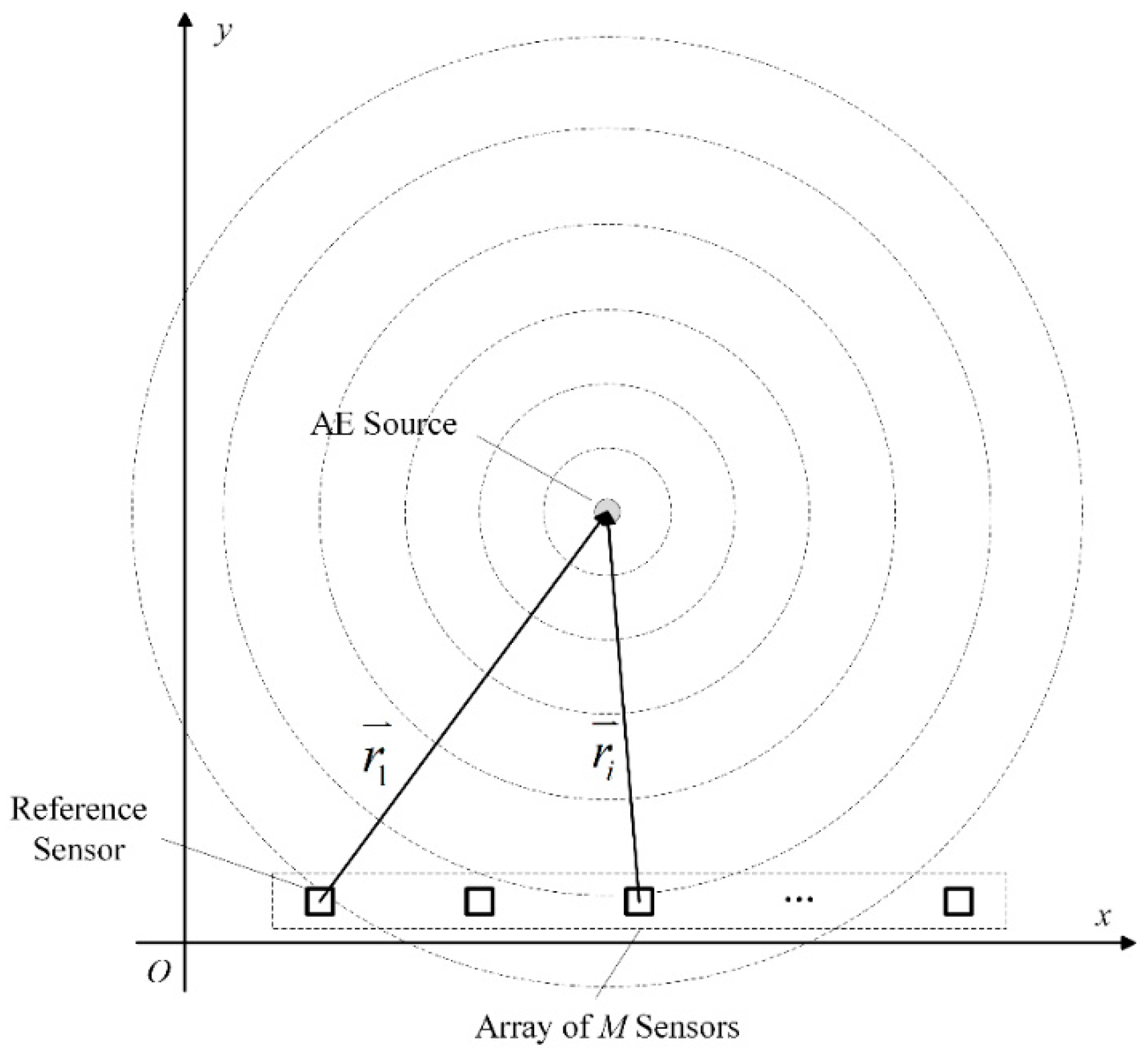
2. Principles
3. Implementation and Test of the Algorithm
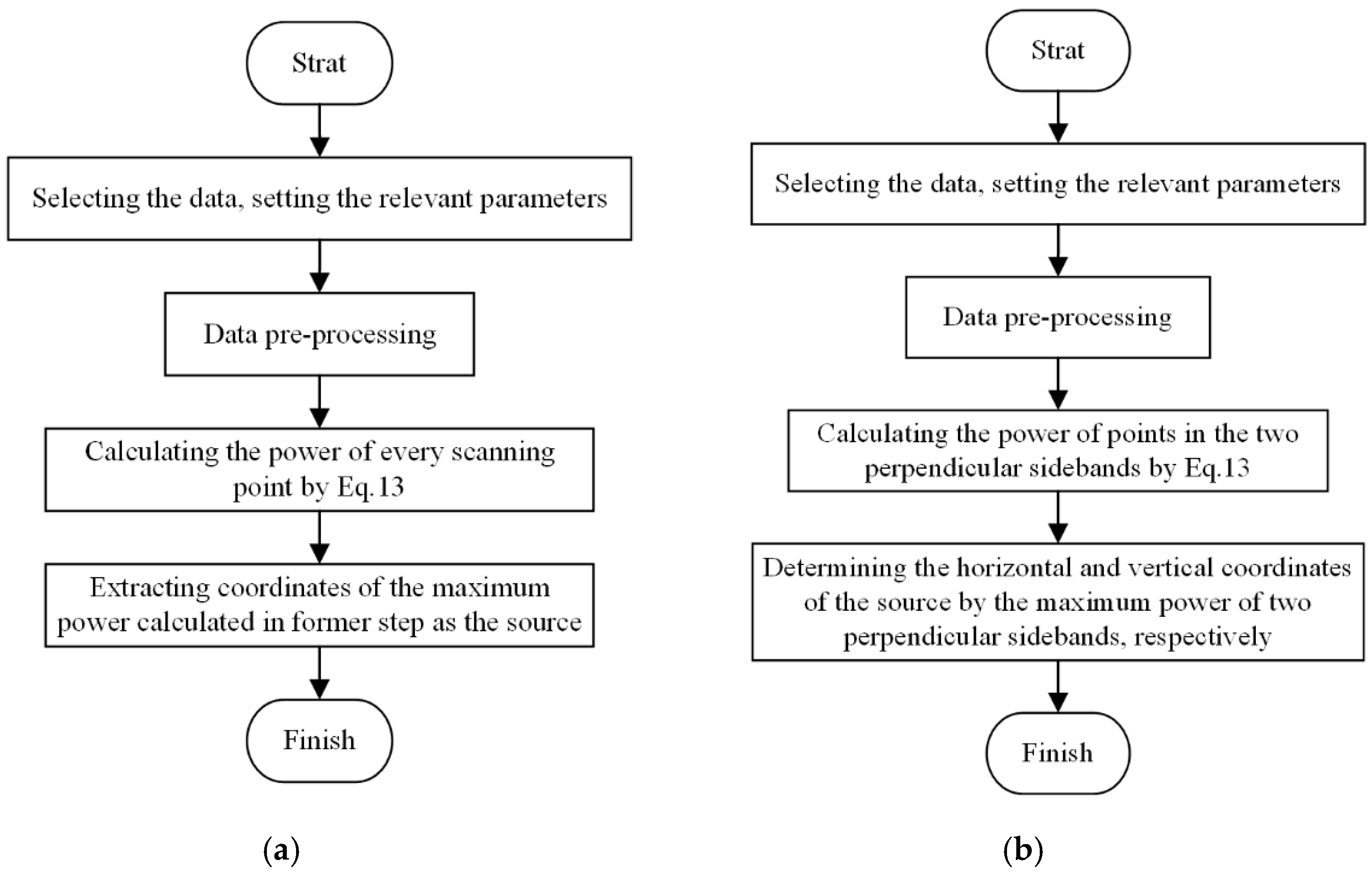
3.1. Implementation and Improvement of the Proposed Algorithm
3.2. Principle of the Fast Algorithm
4. Experimental Verification
5. Conclusions
Author Contributions
Funding
Conflicts of Interest
References
- Mei, H.; Haider, M.F.; Joseph, R.; Migot, A.; Giurgiutiu, V. Recent advances in piezoelectric wafer active sensors for structural health monitoring applications. Sensors 2019, 19, 383. [Google Scholar] [CrossRef] [PubMed]
- Sikdar, S.; Banerjee, S. Structural Health Monitoring of Advanced Composites Using Guided Waves; Stefana, G., Ed.; LAP LAMBERT Academic Publishing: Mauritius, East Africa, 2017; ISBN 978-620-2-02697-0. [Google Scholar]
- Kundu, A.; Eaton, M.J.; Al-jumaili, S.K.; Sikdar, S.; Pullin, R. Acoustic emission based damage localization in composites structures using Bayesian identification. J. Phys. Conf. Ser. 2017, 842, 012081. [Google Scholar] [CrossRef] [Green Version]
- Sikdar, S.; Ostachowicz, W.; Pal, J. Damage-induced Acoustic Emission Source Identification in an Advanced Sandwich Composite Structure. Compos. Struct. 2018, 202, 860–866. [Google Scholar] [CrossRef]
- Sikdar, S.; Mirgal, P.; Banerjee, S.; Ostachowicz, W. Damage-induced acoustic emission source monitoring in a honeycomb sandwich composite structure. Compos. Part B Eng. 2018, 158, 179–188. [Google Scholar] [CrossRef]
- Worden, K.; Manson, G.; Allman, D. Experimental validation of a structural health monitoring methodology: Part I. novelty detection on a laboratory structure. J. Sound Vib. 2003, 259, 323–343. [Google Scholar] [CrossRef]
- Kundu, T. Acoustic Source Localization. Ultrasonics 2014, 54, 25–38. [Google Scholar] [CrossRef] [PubMed]
- Yu, H.S.; Xiao, D.H.; Ma, X.X.; He, T. Near-field beamforming performance analysis for acoustic emission source localization. J. Vibroeng. 2014, 16, 2035–2046. [Google Scholar]
- Ziola, S.M.; Gorman, M.R. Source location in thin plates using cross-correlation. J. Acoust. Soc. Am. 1991, 90, 2551–2556. [Google Scholar] [CrossRef]
- Hamstad, M.A.; Gallagher, A.O.; Gary, J. Examination of the application of a wavelet transform to acoustic emission signals: Part 2. Source location. J. Acoust. Emiss. 2002, 20, 62–82. [Google Scholar]
- Carpinteri, A.; Xu, J.; Lacidogna, G.; Manuello, A. Reliable onset time determination and source location of acoustic emissions in concrete structures. Cem. Concr. Compos. 2012, 34, 529–537. [Google Scholar] [CrossRef]
- Kundu, T.; Nakatani, H.; Takeda, N. Acoustic source localization in anisotropic plates. Ultrasonics 2012, 52, 740–746. [Google Scholar] [CrossRef] [PubMed]
- Park, W.H.; Packo, P.; Kundu, T. Acoustic source localization in an anisotropic plate without knowing its material properties—A new approach. Ultrasonics 2017, 79, 9–17. [Google Scholar] [CrossRef] [PubMed]
- Hensman, J.; Mills, R.; Pierce, S.G.; Worden, K.; Eaton, M. Locating acoustic emission sources in complex structures using gaussian processes. Mech. Syst. Signal Process. 2010, 24, 211–223. [Google Scholar] [CrossRef]
- McCrory, J.P.; Al-Jumaili, S.K.; Crivelli, D.; Pearson, M.R.; Eaton, M.J.; Featherston, C.A.; Guagliano, M.; Holford, K.M.; Pullin, R. Damage classification in carbon fibre composites using acoustic emission: A comparison of three techniques. Compos. Part B 2015, 68, 424–430. [Google Scholar] [CrossRef] [Green Version]
- McLaskey, G.C.; Glaser, S.D.; Grosse, C.U. Beamforming array techniques for acoustic emission monitoring of large concrete structures. J. Sound Vib. 2010, 12, 2384–2394. [Google Scholar] [CrossRef]
- He, T.; Pan, Q.; Liu, Y.G.; Liu, X.D.; Hu, D.Y. Near-field beamforming analysis for AE source localization. Ultrasonics 2012, 5, 587–592. [Google Scholar] [CrossRef] [PubMed]
- He, T.; Xie, Y.; Shan, Y.C.; Liu, X.D. Localizing two acoustic emission sources simultaneously using beamforming and singular value decomposition. Ultrasonics 2018, 1, 3–22. [Google Scholar] [CrossRef] [PubMed]
- Xiao, D.H.; He, T.; Pan, Q.; Liu, X.D.; Wang, J.; Shan, Y.C. A novel acoustic emission beamforming method with two uniform linear arrays on plate-like structures. Ultrasonics 2014, 54, 737–745. [Google Scholar] [CrossRef] [PubMed]
- Huston, R.D. Optimal array configurations for a bartlett beamformer in an arctic environment. J. Acoust. Soc. Am. 1993, 93, 2419. [Google Scholar] [CrossRef]
- Liu, X.D.; Xiao, D.H.; Shan, Y.C.; Pan, Q.; He, T. Solder joint failure localization of welded joint based on acoustic emission beamforming. Ultrasonics 2017, 74, 221–232. [Google Scholar] [CrossRef] [PubMed]


| Speed (m·s−1) | Location | |||||||
|---|---|---|---|---|---|---|---|---|
| AE Sources (mm, mm) | ||||||||
| Set 1 | Set 2 | Set 3 | Set 4 | |||||
| x | y | x | y | x | y | x | y | |
| 270 | 390 | 210 | 450 | 270 | 270 | 390 | 390 | |
| 2000 | 270 | 390 | 210 | 450 | 270 | 270 | 390 | 390 |
| 4000 | 270 | 390 | 210 | 450 | 270 | 270 | 390 | 390 |
| 6000 | 270 | 390 | 210 | 450 | 270 | 270 | 390 | 390 |
| 8000 | 270 | 390 | 210 | 450 | 270 | 270 | 390 | 390 |
| 10,000 | 270 | 390 | 210 | 450 | 270 | 270 | 390 | 390 |
| 12,000 | 270 | 390 | 210 | 450 | 270 | 270 | 390 | 390 |
| Results | AE Sources (mm, mm) | Average Time (s) | |||||||
|---|---|---|---|---|---|---|---|---|---|
| Set 1 | Set 2 | Set 3 | Set 4 | ||||||
| x | y | x | y | x | y | x | y | ||
| 270 | 390 | 210 | 450 | 270 | 270 | 390 | 270 | ||
| BBM | 270 | 390 | 210 | 450 | 270 | 270 | 390 | 270 | 224.38 |
| FBBM | 270 | 390 | 210 | 450 | 270 | 270 | 390 | 270 | 0.72 |
| Speed (m·s−1) | Location | |||||||
|---|---|---|---|---|---|---|---|---|
| AE Sources (mm, mm) | ||||||||
| Set 1 | Set 2 | Set 3 | Set 4 | |||||
| x | y | x | y | x | y | x | y | |
| 270 | 390 | 210 | 450 | 270 | 270 | 390 | 390 | |
| 2000 | 270 | 390 | 210 | 450 | 270 | 270 | 390 | 390 |
| 4000 | 270 | 390 | 210 | 450 | 270 | 270 | 390 | 390 |
| 6000 | 270 | 390 | 210 | 450 | 270 | 270 | 390 | 390 |
| 8000 | 270 | 390 | 210 | 450 | 270 | 270 | 390 | 390 |
| 10,000 | 270 | 390 | 210 | 450 | 270 | 270 | 390 | 390 |
| 12,000 | 270 | 390 | 210 | 450 | 270 | 270 | 390 | 390 |
| Categories of Algorithm | Propagation Speed (m·s−1) | AE Sources (mm, mm) | |||||||
| Set 1 | Set 2 | Set 3 | Set 4 | ||||||
| x | y | x | y | x | y | x | y | ||
| 450 | 450 | 390 | 390 | 210 | 450 | 270 | 390 | ||
| Delay-and-sum beamforming [19] | 2000 | 440 | 450 | 390 | 390 | 210 | 460 | 260 | 390 |
| 2500 | 450 | 460 | 390 | 390 | 200 | 460 | 260 | 390 | |
| 3000 | 450 | 460 | 390 | 390 | 200 | 470 | 260 | 390 | |
| 3500 | 450 | 460 | 390 | 420 | 200 | 470 | 260 | 390 | |
| 4000 | 450 | 460 | 390 | 420 | 200 | 470 | 260 | 390 | |
| Fast Bartlett beamforming | 2000 | 450 | 450 | 390 | 390 | 210 | 450 | 270 | 390 |
| 2500 | 450 | 450 | 390 | 390 | 210 | 450 | 270 | 390 | |
| 3000 | 450 | 450 | 390 | 390 | 210 | 450 | 270 | 390 | |
| 3500 | 450 | 450 | 390 | 390 | 210 | 450 | 270 | 390 | |
| 4000 | 450 | 450 | 390 | 390 | 210 | 450 | 270 | 390 | |
| 6000 | 450 | 450 | 390 | 390 | 210 | 450 | 270 | 390 | |
| 8000 | 450 | 450 | 390 | 390 | 210 | 450 | 270 | 390 | |
| 10,000 | 450 | 450 | 389 | 390 | 210 | 450 | 270 | 390 | |
| 12,000 | 450 | 449 | 390 | 390 | 211 | 449 | 270 | 390 | |
| Categories of Algorithm | Propagation Speed (m·s−1) | Set 5 | Set 6 | Set 7 | Set 8 | ||||
| x | y | x | y | x | x | x | y | ||
| 210 | 210 | 270 | 270 | 450 | 210 | 390 | 270 | ||
| Delay-and-sum beamforming [19] | 2000 | 210 | 250 | 270 | 260 | 470 | 260 | 390 | 290 |
| 2500 | 210 | 240 | 270 | 260 | 470 | 230 | 390 | 260 | |
| 3000 | 210 | 240 | 260 | 260 | 460 | 220 | 390 | 260 | |
| 3500 | 210 | 250 | 260 | 260 | 460 | 220 | 390 | 260 | |
| 4000 | 210 | 250 | 260 | 260 | 460 | 220 | 390 | 270 | |
| Fast Bartlett beamforming | 2000 | 210 | 210 | 270 | 270 | 450 | 210 | 390 | 270 |
| 2500 | 210 | 210 | 270 | 270 | 450 | 210 | 390 | 270 | |
| 3000 | 210 | 210 | 270 | 270 | 450 | 210 | 390 | 270 | |
| 3500 | 210 | 210 | 270 | 270 | 450 | 210 | 390 | 270 | |
| 4000 | 210 | 210 | 270 | 270 | 450 | 210 | 390 | 270 | |
| 6000 | 210 | 210 | 270 | 270 | 450 | 210 | 390 | 270 | |
| 8000 | 210 | 211 | 270 | 270 | 450 | 210 | 390 | 270 | |
| 10,000 | 210 | 208 | 270 | 270 | 450 | 210 | 390 | 270 | |
| 12,000 | 210 | 213 | 270 | 270 | 450 | 210 | 390 | 270 | |
| Scanning Accuracy (mm) | Delay-and-Sum Beamforming (s) | Fast Bartlett Beamforming (s) | Ratio |
|---|---|---|---|
| 5 | 8.49 | 0.17 | 50.69 |
| 2 | 49.16 | 0.35 | 139.96 |
| 1 | 193.26 | 0.72 | 269.49 |
| 0.5 | 780.19 | 2.13 | 366.50 |
| 0.2 | 4887.19 | 11.63 | 420.09 |
© 2019 by the authors. Licensee MDPI, Basel, Switzerland. This article is an open access article distributed under the terms and conditions of the Creative Commons Attribution (CC BY) license (http://creativecommons.org/licenses/by/4.0/).
Share and Cite
Tai, J.; He, T.; Pan, Q.; Zhang, D.; Wang, X. A Fast Beamforming Method to Localize an Acoustic Emission Source under Unknown Wave Speed. Materials 2019, 12, 735. https://doi.org/10.3390/ma12050735
Tai J, He T, Pan Q, Zhang D, Wang X. A Fast Beamforming Method to Localize an Acoustic Emission Source under Unknown Wave Speed. Materials. 2019; 12(5):735. https://doi.org/10.3390/ma12050735
Chicago/Turabian StyleTai, Junfei, Tian He, Qiang Pan, Dayi Zhang, and Xiaoran Wang. 2019. "A Fast Beamforming Method to Localize an Acoustic Emission Source under Unknown Wave Speed" Materials 12, no. 5: 735. https://doi.org/10.3390/ma12050735