Simplification of a Mechanistic Model of Biomass Combustion for On-Line Computations

Abstract

Increasing utilization of intermittent energy resources requires flexibility from energy boilers which can be achieved with advanced control methods employing dynamic process models. The performance of the model-based control methods depends on the ability of the underlying model to describe combustion phenomena under varying power demand. This paper presents an approach to the simplification of a mechanistic model developed for combustion phenomena investigation. The aim of the approach is to simplify the dynamic model of biomass combustion for applications requiring fast computational times while retaining the ability of the model to describe the underlying combustion phenomena. The approach for that comprises three phases. In the first phase, the main mechanisms of heat and mass transfer and limiting factors of the reactions are identified in each zone. In the second phase, each of the partial differential equations from the full scale model are reduced to a number of ordinary differential equations (ODEs) defining the overall balances of the zones. In the last phase, mathematical equations are formulated based on the mass and energy balances formed in the previous step. The simplified model for online computations was successfully built and validated against industrial data.

1. Introduction

Increasing flexibility demands force boilers to operate with wide ranges of load levels and fast transitions between these levels. Model-based control is an excellent technique to achieve optimal load transitions and wide operational ranges. The model-based control methods utilize the process model to obtain a reliable assessment of the key variables of the process state and to predict the future boiler behavior, which is required to ensure extensive control over the combustion process. Thus, further improvement in terms of combustion efficiency and flexibility of boilers demands that the model be able to provide accurate descriptions of combustion phenomena.

Gray-box modeling which comprises ordinary differential equations (ODEs) with parameters identified in order to fit a particular boiler system is a rather popular modeling technique for online applications. For instance, Hogg and El-Rabaie [1] utilized a gray box coal combustion model to develop a generalized predictive control strategy for a 200 MW boiler. Similarly, the most recent application of this technique discusses modelling of boilers of various scales. Bauer et al. [2] developed a gray box model whose structure was based on process knowledge obtained by analyzing mathematical correlations of char combustion. In order to fit the predictions of the model, to the process data empirical coefficients were obtained through model identification. Gölles et al. [3] modeled combustion in a 30 kW boiler using a black-box model to describe the key states present in a boiler. Similarly, Kortela and Jämsä-Jounela [4] used gray-box modeling to model biomass firing in a 16 MW BioGrate boiler. Instead, Flynn and O’Malley [5], constructed a model based on air/mass flows and the adiabatic flame temperature for predicting the key process variables. Although, these models describe the amount of fuel on the grate, they lack important variables such as fuel and gas temperatures which are essential for prediction pollutant emissions.

In mechanistic modeling for real time and control applications two approaches have been presented in the literature. In the first approach, the burning fuel bed of a sloping-grate boiler is represented as a lumped model, developed by Paces and Kozek [6]. The fuel layer is divided in horizontal direction and each lump describes fuel drying, pyrolysis, char combustion and cooling zone. The model comprises gaseous and solid phases and the chemical reactions in these phases are governed by linearized Arrhenius equations. The model developed by Paces and Kozek [6] relied on parameter identification in order to achieve satisfactory accuracy in describing biomass combustion. In the second approach, developed by Belkhir et al. [7], the layer was also divided into gaseous and solid phase, in contrast, only the fuel oxidation reaction was described in the model assuming mass transfer controlled reactions.

Fuzzy logic—neural networks have also been proposed for the modeling of energy boilers [8]. For instance, Peng et al. [9] used a Gaussian radial basis function (RBF), autoregressive model with exogenous inputs (ARX) to describe combustion in a coal-fired boiler for the development of a nonlinear model predictive control strategy for efficiency improvement of the de-NO_x reaction. This approach proved to be effective in minimizing ammonia consumption in the de-NO_x reaction. The main approach of describing fuel combustion in ARX models is to relate fuel and air flows to boiler power output [10] or to steam production [11,12].

The models proposed for on-line applications can be divided into two categories based on the degree of involvement of identification methods: (1) fully data-based methods—ARX, ANN-ARX, ANN-fuzzy; and (2) models based on ODEs with identified parameter functions. Nevertheless, both these model categories suffer from limitations, such as data-overfitting and insufficient reproducibility of nonlinear process behavior. In addition, industrial processes tend to operate at a limited number of regimes and thus the identification of less frequently occurring operational conditions is inherently difficult. For non-linear processes, such as biomass combustion, mechanistic modeling is the only method which can guarantee acceptable accuracy and robustness, since non-linear system identification suffers from several shortcomings. Morari and Lee [13] highlighted numerous issues related to nonlinear model identification, such as model structure determination, test input signal design, multiple input-multiple output model fitting algorithm and uncertainty quantification for robust control. However, mechanistic models developed for real time applications neglect important phenomena such as moisture evaporation due to convective and radiative heat transfer which is particularly important in case of moist biomass fuel and in boiler operating under concurrent combustion conditions and overfed fuel beds where hot char comes into contact with moist cold fuel.

On the other hand, several mechanistic models were developed for process phenomena investigation that accurately reproduce the process behavior. Unfortunately, these models are excessively detailed and contain variables and phenomena which have insignificant impact on the descriptive ability of the model. Moreover, in these mechanistic models, all parts of the burning fuel layer are described equally in detail, even the ones which remain at constant conditions for the long duration of time and do not affect the overall burning behavior of a fuel layer. Thus, by only describing the relevant phenomena and the parts of the fuel layer, a significant reduction in the model complexity can be achieved which leads to simpler model implementation, calibration, short computational times and consequently considerably lower hardware requirements which is especial relevant for industrial control systems.

The aim of this study is to simplify mechanistic model to decrease the excessive complexity while retaining the ability of a model to describe combustion phenomena. With the method, we determine the factors, such as heat and mass transfer mechanisms having the largest impact on the model accuracy and disregard the factors with low contribution. In addition, based on the method, we divide the layer into a few zones which eliminates the need for the spatial discretization of the model and considerably shortens the computational time. Based on this, we obtain a novel dynamic combustion model which provides the insight into the burning fuel layer with accuracy comparable to that of the original model, but with a simpler mathematical formulation and significantly shorter computational times. The simplified model was evaluated against the original mechanistic model to ensure its ability to describe combustion phenomena. Furthermore, the model developed in this work has been successfully validated against industrial data from a BioGrate boiler suggesting the applicability of the proposed simplification approach. As a result, this work finally closes the gap between the detailed modeling of biomass combustion for phenomena investigation and the modeling of combustion processes for applications which include process control and monitoring.

The remainder of the paper is structured as follows. Section 2 describes a BioGrate process. Section 3 presents the simplification approach along with the description of the model upon which simplification is based and the simplified model validation. In Section 4, the simplified model is compared against the original and a linear one. Conclusions and future research are presented in Section 5.

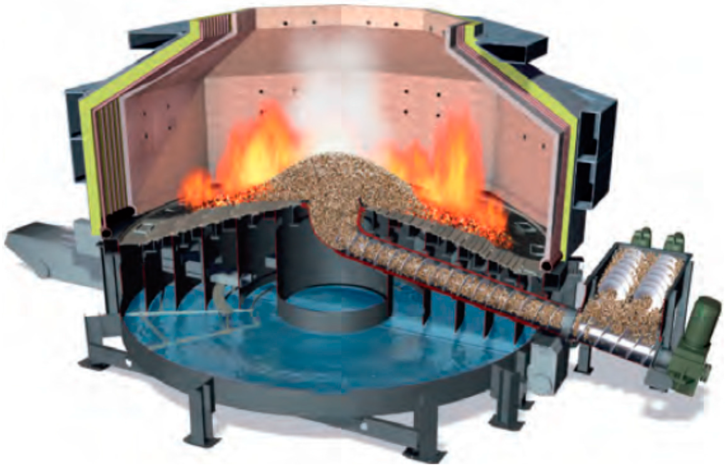
2. Process Description of a BioGrate Boiler

The BioGrate boiler is used for electricity and steam production as well as to supply heat to a local municipal hot water network. BioGrate boilers are based on a conical grate technology that is designed to utilize various fuels with high moisture content. A BioGrate furnace consists of the following functional parts: grate rings, a water-filled ash space below the grate and heat-insulating refractory walls around the grate rings which form the combustion chamber.

To improve the spread of fuel within the combustion chamber, the grate consists of several ring zones, which are further divided into two types of alternating rings: rotating and fixed. Half the rotating rings move clockwise and the rest counter clockwise, distributing the fuel evenly on the grate. As the fuel is fed into the center of the grate from below, the surface of the fuel starts to dry in the center of the cone as a result of heat radiation, which is emitted by the combusting flue gas and reflected back to the grate by the grate walls. The dry fuel then proceeds to the outer rings of the grate, where pyrolysis char gasification and combustion occur. Finally, the resulting ash and carbon residues fall off the edge of the grate into the water-filled annular ash space and Figure 1 shows an outline of a BioGrate furnace.

The air required for combustion is distributed via annular primary air registers below the grate to the nozzles in each grate plate (primary air) and through nozzles in the combustion chamber wall (secondary air). Burning produces heat that is absorbed in several steps: first, the evaporator and water-tube walls of the boiler absorb the energy from the flue gases, which is followed by energy transfer to steam through superheaters. In the third phase, heat is transferred from the flue gas to the feed water by the convective evaporator, before finally the economizers remove the remaining flue-gas energy.

3. Model Development for Process Control and Monitoring

Model development for process control and monitoring purposes proceeds through the simplification of a mechanistic model. Therefore, this section is divided into three main parts. Firstly, the mechanistic model developed by the authors [14,15] is presented, including proposed simplifications based on the subsequent simulation results. The simplified model is then presented and discussed prior to the last section which outlines the validation of the developed model.

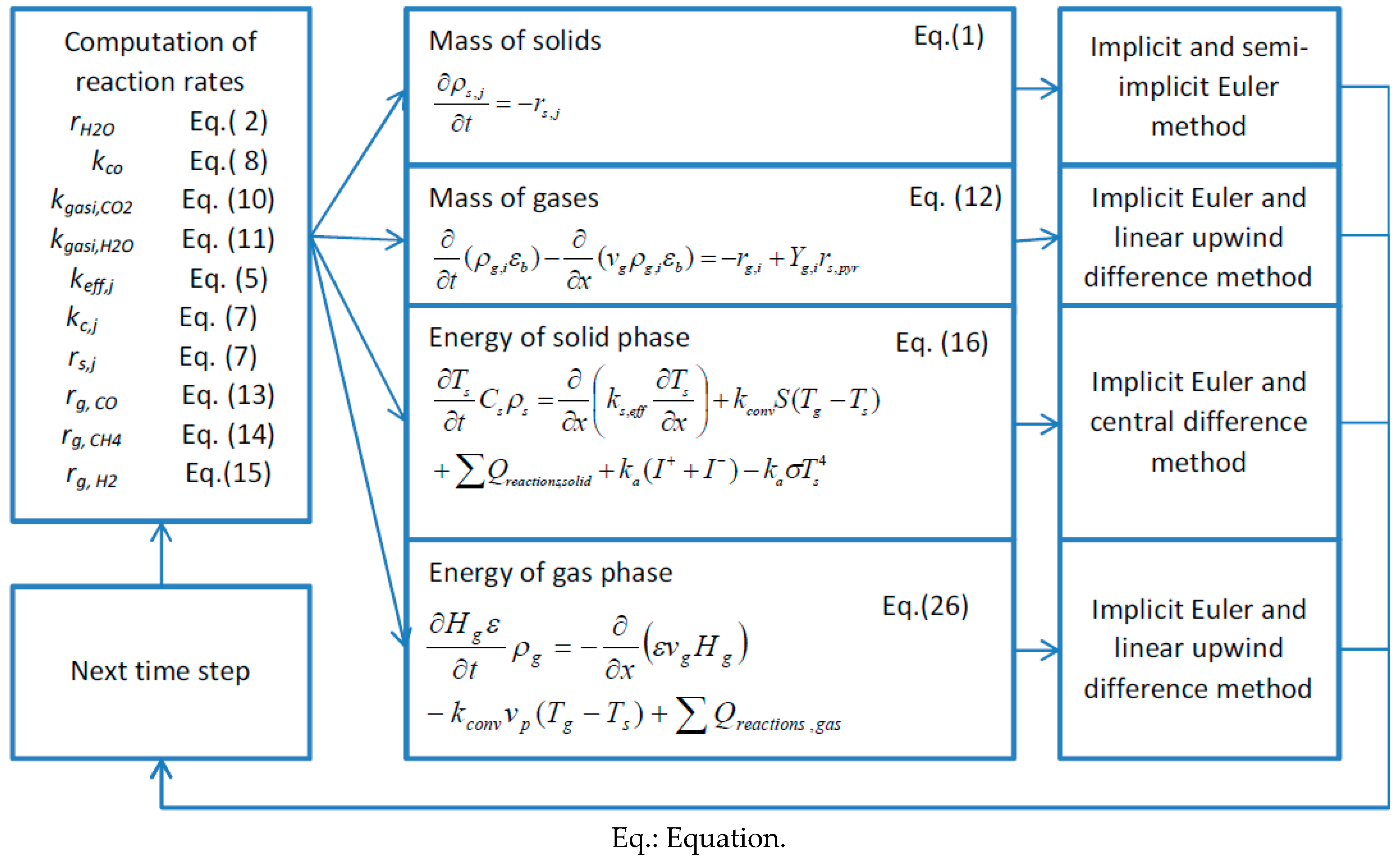
3.1. Mechanistic Model

In a BioGrate boiler, reactions of biomass occur through three main reaction pathways that can take place either in parallel or sequentially with respect to each other: drying, pyrolysis and char conversion and the mechanistic modeling of the BioGrate boiler considers these three stages of the biomass combustion. As the model accounts for mass and energy conservation, it considers two phases, a solid and a gaseous one. The burning fuel bed in a BioGrate boiler is modeled in one dimension using the walking grate concept [14]. The walking grate approach divides the fuel layer into vertical, one-dimensional portions with the fuel movement on a grate assumed to resemble that observed on a traveling grate. As a result, the developed model describes traveling grate combustion and the structure of the model with the solving algorithm is presented in Figure 2.

3.1.1. Modelling of Mass Conservation in the Solid Phase

The solid phase reactions considered by the model include drying, pyrolysis as well as char oxidation and gasification. In general, these can be described by Equation (1) and the reactions considered in the solid phase are presented in

Table 1. Solid phase reactions.

${\mathrm{H}}_2\mathrm{O}\left(\mathrm{l}\right)\stackrel{\phantom{\hspace{1em}\hspace{1em}}}{\to }{\mathrm{H}}_2\mathrm{O}\left(\mathrm{g}\right)$

$\mathrm{Wood}\stackrel{\phantom{\hspace{1em}\hspace{1em}}}{\to }\mathrm{Gas},\mathrm{Tar},\mathrm{Char}$

$\mathrm{C}\left(\mathrm{s}\right)+{\mathsf{\alpha }\mathrm{O}}_2\left(\mathrm{g}\right)\stackrel{\phantom{\hspace{1em}\hspace{1em}}}{\to }2(1-\mathsf{\alpha })\mathrm{CO}\left(\mathrm{g}\right)+(2\mathsf{\alpha }-{1)\mathrm{CO}}_2(\mathrm{g})$

$\mathrm{C}\left(\mathrm{s}\right)+{\mathrm{CO}}_2\left(\mathrm{g}\right)\stackrel{\phantom{\hspace{1em}\hspace{1em}}}{\to }2\mathrm{CO}\left(\mathrm{g}\right)$

$\mathrm{C}\left(\mathrm{s}\right)+{\mathrm{H}}_2\mathrm{O}\left(\mathrm{g}\right)\stackrel{\phantom{\hspace{1em}\hspace{1em}}}{\to }\mathrm{CO}\left(\mathrm{g}\right)+{\mathrm{H}}_2\left(\mathrm{g}\right)$

:

$$\frac{\partial {\mathsf{\rho }}_{\mathrm{s},j}}{\partial t}=-r_{\mathrm{s},j}$$

(1)

The rate of drying, Equation (2), is defined by the energy available for evaporation:

$$r_{{\mathrm{s},\mathrm{H}}_2\mathrm{O}}=\max \left(0,\frac{{\mathsf{\rho }}_{{\mathrm{H}}_2\mathrm{O}}}{{\max (\mathsf{\rho }}_{{\mathrm{H}}_2\mathrm{O}})}\frac{C_{\mathrm{s}}(T_{\mathrm{s}}-378(\mathrm{K}))}{\Delta t\Delta H_{\mathrm{evap}}}\right)$$

(2)

The pyrolysis reaction rates are described by Equations (3) and (4). The volatile matter of the fuel was assumed to contain two pseudo-components with different combination of cellulose, lignin and hemicellulose. The first component mainly contains lignin and slowly decomposes over a large range of temperatures while the second contains mainly cellulose and hemicellulose. The mass fraction of the first volatile component in wood is 0.15.

$$r_{\mathrm{s},\mathrm{pyr},1}=315.6\exp (-80(\mathrm{kJ}/\mathrm{mol})/(R{T}_{\mathrm{s}})){\mathsf{\rho }}_{\mathrm{pyr},1}$$

(3)

$$r_{\mathrm{s},\mathrm{pyr},2}=2.205\cdot {10}^4\exp (-78(\mathrm{kJ}/\mathrm{mol})/(R{T}_{\mathrm{s}})){\mathsf{\rho }}_{\mathrm{pyr},2}$$

(4)

Pomerantsev [16] has proposed to calculate the rate of char burning as a function of either char or oxygen concentration, depending on whichever is limiting. Thus the rates for the char reactions can be calculated by Equation (5):

$$r_{\mathrm{s},i}=k_{\mathrm{eff},i}{\mathsf{\rho }}_{\mathrm{g},i}$$

(5)

For each heterogeneous char reaction, an effective reaction constant—given by Equation (6)—is then calculated as follows:

$$k_{\mathrm{eff},i}=\frac{S{k}_{\mathrm{m},i}{k}_{\mathrm{r},i}}{S{k}_{\mathrm{m},i}+k_{\mathrm{r},i}}$$

(6)

where S is the density number, the particle surface area per unit volume [17], given by Equation (7), k_m,i is the mass transfer coefficient [17], calculated from Equation (8) and k_r,i is the reaction constant:

$$S=\frac{6\left(1-{\mathsf{\epsilon }}_{\mathrm{b}}\right)}{d_{\mathrm{p}}}$$

(7)

where ε_b is the fuel bed porosity and d_p is the particle diameter.

$$k_{\mathrm{m},i}=D_{\mathrm{g},i}/d_{\mathrm{p}}\left(2+{\mathrm{Re}}^{1/2}S{c}^{1/3}\right)$$

(8)

The reaction constants, k_r,i, are determined for three different chemical reactions: oxidation, Equation (9) [18], and reduction with H₂O, Equation (10) [19], and CO₂, Equation (11) [20]:

$$k_{\mathrm{r},\mathrm{C}}=1.1\cdot {10}^6\cdot \exp \left(-114.5(\mathrm{kJ}/\mathrm{mol})/R/T_{\mathrm{s}}\right)$$

(9)

$$k_{{\mathrm{r},\mathrm{H}}_2\mathrm{O}}=9.99\cdot {10}^4\cdot \exp \left(-136(\mathrm{kJ}/\mathrm{mol})/R/T_s\right)\left(1-X\right)\sqrt{1-10\ln (1-X)}$$

(10)

$$k_{\mathrm{r},\hspace{0.17em}{\mathrm{CO}}_2}=1.1\cdot {10}^9\exp \left(-260(\mathrm{kJ}/\mathrm{mol})/R/T_{\mathrm{s}}\right)X$$

(11)

with the associated CO/CO₂ ratio given by Equation (12) [21]:

$${\mathrm{CO}/\mathrm{CO}}_2=4.3\exp (-3390/T_{\mathrm{s}})$$

(12)

3.1.2. Modelling of Mass Conservation in the Gas Phase

The gas phase modelling, presented in Equation (13), describes gas convection, combustion of carbon monoxide (Equation (14)), methane (Equation (15)) [16] and hydrogen (Equation (16)) [16], as well as gas formation in the pyrolysis reaction, Y_g,ir_pyr:

$$\frac{\partial }{\partial t}({\mathsf{\rho }}_{\mathrm{g},i}{\mathsf{\epsilon }}_b)-\frac{\partial }{\partial x}(v_{\mathrm{g}}{\mathsf{\rho }}_{\mathrm{g},i}{\mathsf{\epsilon }}_b)=-r_{\mathrm{g},i}+Y_{\mathrm{g},i}{r}_{\mathrm{pyr}}$$

(13)

where r_pyr is the pyrolysis reaction rate, while Y_g,i is the mass fraction of the gaseous pyrolysis product formed:

$$r_{\mathrm{g},\mathrm{CO}}=1.3\cdot {10}^{14}\exp (-125.5(\mathrm{kJ}/\mathrm{mol})/R/T_{\mathrm{g}})\hspace{0.17em}{C}_{\mathrm{CO}}\hspace{0.17em}{C_{{\mathrm{O}}_2}}^{0.5}\hspace{0.17em}{C_{{\mathrm{H}}_2\mathrm{O}}}^{0.5}$$

(14)

$$r_{{\mathrm{g},\mathrm{CH}}_4}=5.6\cdot {10}^{12}\exp (-103.8(\mathrm{J}/\mathrm{mol})/R/T_{\mathrm{g}})\hspace{0.17em}{C}_{{\mathrm{O}}_2}$$

(15)

$$r_{{\mathrm{g},\mathrm{H}}_2}=2.14\cdot {10}^{14}\exp (-129\text{\hspace{0.17em}}(\mathrm{J}/\mathrm{mol})/R/T_{\mathrm{g}})\hspace{0.17em}{C}_{{\mathrm{O}}_2}$$

(16)

The following gaseous components are considered by the model: water vapor, tar, oxygen, carbon monoxide, carbon dioxide, nitrogen, methane, and hydrogen.

3.1.3. Modelling of Energy Conservation in the Solid Phase

The energy equation for the solid phase describes heat conduction, heat exchange between the phases, energy consumed in the drying and pyrolysis reactions and energy gained by char combustion (Equation (17)):

$$\frac{\partial T_{\mathrm{s}}}{\partial t}{C}_{\mathrm{s}}{\mathsf{\rho }}_{\mathrm{s}}=\frac{\partial }{\partial x}\left({\mathsf{\kappa }}_{\mathrm{s},\mathrm{eff}}\frac{\partial T_{\mathrm{s}}}{\partial x}\right)+k_{\mathrm{conv}}S(T_{\mathrm{g}}-T_{\mathrm{s}})+{\displaystyle \sum Q_{\mathrm{s},i}}+k_{\mathrm{a}}(I^{+}+I^{-})-k_{\mathrm{a}}\mathsf{\sigma }{T}_{\mathrm{s}}^4$$

(17)

The heat conduction in solid particles is described by Equations (18)–(23) [22]:

$${\mathsf{\kappa }}_{\mathrm{s},\mathrm{eff}}={\mathsf{\epsilon }}_{\mathrm{p}}{k}_{\max }+(1-{\mathsf{\epsilon }}_{\mathrm{p}})k_{\min }+k_{\mathrm{s},\hspace{0.17em}\mathrm{rad}}$$

(18)

$$k_{\mathrm{s},\mathrm{rad}}=\frac{4{\mathsf{\epsilon }}_{\mathrm{p}}\mathsf{\sigma }{T_{\mathrm{s}}}^3{d}_{\mathrm{cavity}}}{1-{\mathsf{\epsilon }}_{\mathrm{p}}}$$

(19)

$$d_{\mathrm{cavity}}=3.5\cdot {10}^{-5}\sqrt{{\mathsf{\epsilon }}_{\mathrm{p}}}$$

(20)

$${\mathsf{\epsilon }}_{\mathrm{p}}=1-({\mathsf{\rho }}_{\mathrm{v}}+{\mathsf{\rho }}_{\mathrm{c}})/1500-{\mathsf{\rho }}_{\mathrm{w}}/1000$$

(21)

$$k_{\min }=\frac{k_{\mathrm{g}}{k}_{\mathrm{fiber}}}{{\mathsf{\epsilon }}_{\mathrm{p}}{k}_{\mathrm{fiber}}+(1-{\mathsf{\epsilon }}_{\mathrm{p}})k_{\mathrm{g}}}$$

(22)

$$k_{\max }={\mathsf{\epsilon }}_{\mathrm{p}}{k}_{\mathrm{g}}+(1-{\mathsf{\epsilon }}_{\mathrm{p}})k_{\mathrm{fiber}}$$

(23)

The radiative heat transfer inside the bed is described with a two-flux model given by Equations (24) and (25), where the absorption and scattering coefficients are given by Equation (26) [23]:

$$\frac{\mathrm{d}{I}^{+}}{\mathrm{d}x}=-(k_{\mathrm{a}}+k_{\mathrm{s}})I^{+}+k_{\mathrm{s}}{I}^{-}+\frac{1}{2}{k}_{\mathrm{a}}\mathsf{\sigma }\hspace{0.17em}{T}_{\mathrm{s}}^4$$

(24)

$$-\frac{\mathrm{d}{I}^{-}}{\mathrm{d}x}=-(k_{\mathrm{a}}+k_{\mathrm{s}})I^{-}+k_{\mathrm{s}}{I}^{+}+\frac{1}{2}{k}_{\mathrm{a}}\mathsf{\sigma }\hspace{0.17em}{T}_{\mathrm{s}}^4$$

(25)

$$k_{\mathrm{a}}=-\frac{1}{d_{\mathrm{p}}}\ln ({\mathsf{\epsilon }}_{\mathrm{b}}),\hspace{0.17em}{k}_{\mathrm{s}}=0$$

(26)

3.1.4. Modelling of the Gas Phase Energy Conservation

The energy continuity equation—Equation (27)—of the gas phase considers the heat exchange between the gas and solid phases, the energy received through gas convection, and the energy gained from carbon monoxide, methane and hydrogen oxidation:

$$\frac{\partial H_{\mathrm{g}}{\mathsf{\epsilon }}_{\mathrm{b}}}{\partial t}{\mathsf{\rho }}_{\mathrm{g}}=-\frac{\partial }{\partial x}\left({\mathsf{\epsilon }}_{\mathrm{b}}{v}_{\mathrm{g}}{H}_{\mathrm{g}}\right)-k_{\mathrm{conv}}S(T_{\mathrm{g}}-T_{\mathrm{s}})+{\displaystyle \sum Q_{\mathrm{g},i}}$$

(27)

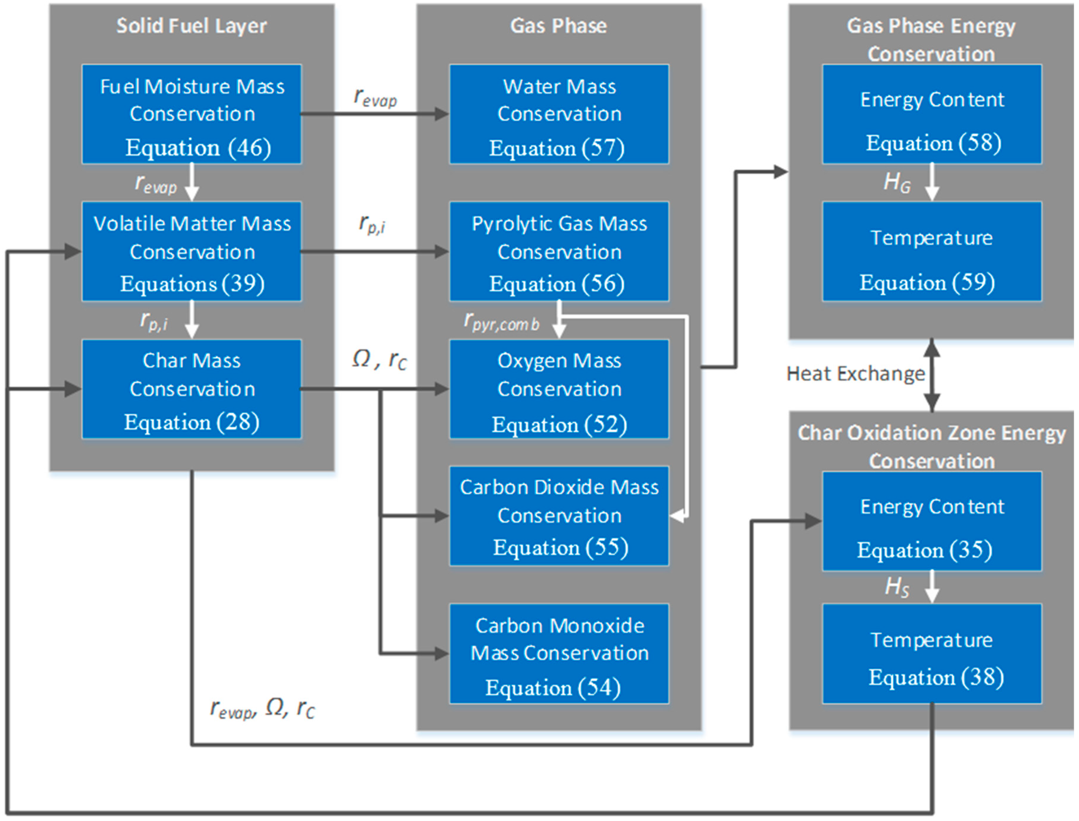
3.2. Development of a Simplified Dynamic Model

The main idea of the simplification is to divide the fuel layer into zones, located between the reaction fronts, and to assume uniform conditions within each zone. This is based on the observation that large temperature and composition gradients exist at the reaction fronts while the degree of variation is limited in between the fronts. Such an approach allows a significant reduction in the number of variables by neglecting the ones which are not critical in a mathematical description of a combustion process.

Simplification of the model developed in this study involves the following three main phases. In the first phase, the main mechanisms of heat and mass transfer and limiting factors of the reactions, such as oxygen concentration and the energy available, are identified in each zone. In the seconds phase, each of the partial differential equations from the full scale model, representing conservation laws at each spatial point, are reduced to a number of ODEs defining the overall balances of the zones. In the last phase, mathematical equations are formulated based on the mass and energy balances formed in the previous step.

3.3. Approach for Simplification of the Mechanistic Model

The simplification of the model developed in this work involves three main phases. The purpose of the first phase is to divide the fuel layer into zones to reduce computational time. This is performed based on the simulation results from the mechanistic model by identifying largest gradients with respect to the char, volatile and moisture content which indicate the end of each respective zone.

In the second phase, the reaction-limiting factors are determined among oxygen concentration, convective, radiative and conductive heat transfer, such that non-restrictive factors can be omitted from the model. This is done by comparing the magnitude of each heat transfer mechanism with respect to each other and by removing the least significant ones. The char oxidation reaction is generally known to be limited by the primary air feed, since almost all oxygen is consumed close to the grate and hence the propagation of the front is limited by oxygen supply [15]. The area on top of the fuel layer is not included into the consideration, since it does not receive oxygen from below. With the absence of oxygen, the low heat conductivity of char can be assumed to prevent the heat flux downwards and to effectively stop the front from propagating. In case of pyrolysis and drying, the front propagation of these reactions is limited by heat transfer from hotter areas as these reactions require sufficient temperature to become active. Thus, the identification of reaction limiting factors can be done based on the gradients in the temperature profile as well as on the radiative heat flux profile.

These considerations result in a significant simplification of the temperature profile as only the temperature of the char layer is assumed to be a variable. Instead, concentration-wise the fuel layer is divided into three zones. This results in a great reduction in computational time by avoiding the need for spatial discretization which results in a significant decrease in the number of equations to be solved.

Finally, the detailed description of the third phase of the simplification approach, namely, the mathematical formulation of the model, is provided in the following.

3.4. Mathematical Formulation of the Simplified Model

This section presents the development of a simplified dynamic model for on-line computations. First, based on the simulation results from the enhanced model the reaction-limiting factors are identified. Then, the equations of the enhanced model are simplified by considering these factors and the model is validated. The simplified model was implemented in the MATLAB computation environment and solved with the implicit Euler method. An overview of the model structure is presented in Figure 3.

Mathematical Formulation of the Dynamic Model for On-Line Computations

In the first phase, the reaction-limiting factors have to be identified, which is done based on simulations of the enhanced mechanistic model. The results from the mechanistic model (Figure 4) suggest the presence of three reaction fronts corresponding to each major reaction: char combustion, pyrolysis, and evaporation zones. This means that the walking grate concept, which described fuel movement on the grate and the temperature and concentration gradients in the horizontal direction in the dynamic model, has to be omitted because of the assumption of uniform conditions inside each zone.

In the second phase, the reaction-limiting factors are identified from the simulation results presented in Figure 4 starting from char oxidation zone. In that zone, oxygen is consumed almost completely by the oxidation reaction. However, the primary air flow initially decreases the temperature of char as it enters the furnace. This effect is shown in Figure 4 as a decrease in temperature which becomes more significant towards the surface of the grate. Thus, in addition to the oxidation reaction also the heat exchange between char and the primary air is significant and can be up to 1000 °C close to the grate.

The pyrolysis zone, which lies above the char oxidation zone, is rather thin and, thus, the temperature of the reacting fuel is close to the char combustion temperature. The simulation results in Figure 4 indicate that the char oxidation and pyrolysis zones overlap since char forms during the devolatilization reaction. Thus, it is assumed that the temperature of the pyrolysis zone equals that of the char oxidation zone.

Moisture evaporation, being an endothermic reaction, is limited by the radiative as well as by the convective heat transfer from the char combustion zone. The heat conduction is neglected due to its low contribution since, conductive heat flux over one char particle and 100 °C temperature gradient is 670 W/m² while in case of radiative heat transfer it is nine times higher (calculated by differentiating the heat flux over the interface between the drying and pyrolysis zones over one particle diameter). However, conduction contributes only slightly to the evaporation due to low heat conductivity of char and thus its effect is neglected. The contribution of the radiative heat transfer mechanism is only significant at the interface of the pyrolysis and the drying zones where temperature exceeds 500 °C. Thus, both heat transfer mechanisms can be assumed to contribute to the moisture evaporation. Next, mathematical equations based on these considerations are presented for each zone, in accordance with the phase three of the approach.

• Char Combustion Zone

In char combustion zone, both the mass and energy are considered in accordance with the general simplification approach.

• Mass Conservation

Char forms during the pyrolysis phase in which cellulose, hemicellulose and lignin decompose to produce volatile gas and char which is subsequently consumed by the oxidation reaction:

$$\frac{\mathrm{d}m{}_{\mathrm{C}}}{\mathrm{d}t}=X_{\mathrm{C}}{\displaystyle \sum _{i=1}^3{r}_{\mathrm{p},i}}-r_{\mathrm{C}}$$

(28)

where m_C is the amount of char on the grate, X_C is the char yield from wood pyrolysis and r_C is the char reaction rate, r_p,i accounts for individual pyrolysis reactions of cellulose, lignin and hemicellulose. The effective char consumption rate is described by Equation (29) and, depending on the conditions, char oxidation is kinetically or mass transfer controlled. Owing to the omission of the spatial coordinates, the term h_CSV was introduced to model the effect of the char layer thickness on the consumption of oxygen. Thus, Equation (29), which describes the effective rate constant of char combustion, assuming that the process can be both reaction and mass transfer controlled, in the mechanistic model, is modified as:

$$k{}_{\mathrm{C},\mathrm{eff}}=h{}_{\mathrm{C}}SVk{}_{{\mathrm{O}}_2}{k}_{\mathrm{C}}/(k_{\mathrm{C}}+h_{\mathrm{C}}SV{k}_{{\mathrm{O}}_2})$$

(29)

where k_C,eff is the effective reaction rate of char, V is the fuel layer volume, k_O2 is the mass transfer coefficient of oxygen onto the surface of char particle, h_C is the mass fraction of char on the grate where the mass transfer coefficient is calculated from the Sherwood number:

$$k_{{\mathrm{O}}_2}=D_{\mathrm{g}}/d_{\mathrm{p}}\left(2+{\mathrm{Re}}^{1/2}S{c}^{1/3}\right)$$

(30)

where D_g is the oxygen diffusivity in air, and d_p is the particle size

The volume of the fuel layer is defined by Equation (31), which assumes that both fuel and char contribute to the overall volume of the fuel bed:

$$V=\frac{m_{\mathrm{fuel}}}{{\mathsf{\rho }}_{\text{fuel}\hspace{0.17em}\text{bed}\hspace{0.17em}\text{dry}}}+\frac{m_{\mathrm{C}}}{{\mathsf{\rho }}_{\mathrm{char}\hspace{0.17em}\mathrm{bed}}}$$

(31)

where ρ_{fuel bed dry} is the density of dry fuel, and ρ_{char bed} is the density of char bed

Parameter S is the density number which describes surface to volume ratio of the fuel layer:

$$S=\frac{6(1-\mathsf{\epsilon })}{d_{\mathrm{p}}}$$

(32)

where ε is the porosity of fuel bed and h_C is the mass fraction of char:

$$h_{\mathrm{C}}=m_{\mathrm{C}}/(m_{\mathrm{fuel}}+m_{{\mathrm{H}}_2\mathrm{O},\mathrm{l}}+m_{\mathrm{C}})$$

(33)

where m_C, m_fuel and m_H2O,l are the amounts of char, fuel and water, respectively. Thus the term h_CSV in Equation (29) effectively describes the overall surface area of char available for the oxidation reaction.

The char combustion kinetics are defined by Equation (34) [24]:

$$k_{\mathrm{C}}=1.1\cdot {10}^6\exp (-114.5(\mathrm{kJ}/\mathrm{mol})/(R{T}_{\mathrm{S}})$$

(34)

• Energy Conservation

The energy balance of the solid phase, as outlined in Equation (35), includes the energy content of char and of minute amounts of volatile components and depends on the energy lost due to emitted radiation and heat transferred to the incoming primary air flow. A fraction of the energy of the solid phase is transferred with the gases formed in pyrolysis and oxidation reactions. Moreover, the enthalpy of the solid phase is increased by oxidation reactions and heat from pyrolysis reactions. As the air is supplied from under the grate, it is heated by the burning char layer, such that:

$$\frac{\mathrm{d}{H}_{\mathrm{S}}}{\mathrm{d}t}=Q_{\mathrm{in}}-Q_{\mathrm{out}}-\Delta H_{\mathrm{evap}}{r}_{\mathrm{evap},\mathrm{rad}}+{\displaystyle \sum _{i=1}^3\left(\Delta H_{\mathrm{p},i}-C_{\mathrm{p},\mathrm{w}}T\right)\hspace{0.17em}{r}_{\mathrm{p},i}+Q_{\mathrm{C}}-Ah(T_{\mathrm{S}}-T_{\mathrm{G},\mathrm{In}})}$$

(35)

where Q_in is the energy of contained in primary air, Q_out is the energy of the gas out flow, ∆H_s is the enthalpy of the solid phase, ∆H_p,i is the pyrolysis heat of component i, C_p,w is the heat capacity of wood, Q_C is the energy form char combustion, A is the total outer surface of the fuel, and h is the heat transfer coefficient.

It is evident from the Equation (35) that depending on the intensity of thermal decomposition, the effect of pyrolysis heat can have a significant effect on the energy balance and thus needs to be estimated. Moreover, the overall pyrolysis enthalpy is fuel specific and is largely dependent on chemical composition of fuel and can be endothermic, neutral or exothermic. The endothermicity or exothermicity is essentially defined by the pyrolytic secondary reactions. In case of the debarking residue used as fuel in BioGrate boiler the pyrolysis heats for cellulose, lignin and hemicellulose were determined to be −100, −600 and −200 kJ/mol, respectively [25]. These are the total reaction heats which include the heat from primary and secondary reactions for each component. Modeling of lignin decomposition is, especially, important since it decomposes slowly and the pyrolysis temperature can increase up to 900 °C before lignin has completely decomposed. In contrast, hemicellulose and cellulose complete decomposition at relatively moderate temperatures.

The char is assumed to react to carbon monoxide and carbon dioxide and the overall energy contribution is described by Equation (36):

$$Q_{\mathrm{C}}=\left(\frac{\Delta H_{\mathrm{CO}}}{M_{\mathrm{CO}}}\frac{2(\Omega -1)}{\Omega }{r}_{\mathrm{C}}+\frac{\Delta H_{{\mathrm{CO}}_2}}{M_{{\mathrm{CO}}_2}}\frac{2-\Omega }{\Omega }-C_{\mathrm{p},\mathrm{C}}{T}_{\mathrm{S}}\right)r_{\mathrm{C}}$$

(36)

where ∆H_CO and ∆H_CO2 is the reaction enthalpy of char oxidation to carbon monoxide and carbon dioxide, respectively, C_p,c is the heat capacity of char, Ω is the stoichiometric coefficient.

The coefficient is given by Equation (37) [21]. This equation accounts for the fact that at high temperatures the breakage of oxygen-carbon complex on the surface of the char particle tends to produce mostly CO [16]:

$$\Omega =\frac{2+2\cdot 4.3\exp \left(-3390/T_{\mathrm{S}}\right)}{2+4.3\exp \left(-3390/T_{\mathrm{S}}\right)}$$

(37)

The temperature of the solid phase can be calculated by dividing the energy content of the char by its enthalpy:

$$T=\frac{H_{\mathrm{S}}}{m_{\mathrm{C}}{C}_{\mathrm{p},\mathrm{c}}+C_{\mathrm{p},\mathrm{w}}{\displaystyle \sum _i^3{m}_{\mathrm{p},i}}}$$

(38)

• Fuel Pyrolysis Zone

For each volatile component of the fuel (cellulose, hemicellulose, and lignin), the following mass conservation equation is devised:

$$\frac{\mathrm{d}{m}_{\mathrm{p},i}}{\mathrm{d}t}=r_{\mathrm{evap}}\frac{X_{\mathrm{p},i}(1-X_{\mathrm{m}})}{X_{\mathrm{m}}}-r_{\mathrm{p},i}$$

(39)

where X_p,i is the fraction of cellulose, hemicellulose and lignin, X_m, the moisture content of the fuel in the furnace, is defined by Equation (40):

$$X_{\mathrm{m}}=\frac{m_{{\mathrm{H}}_2\mathrm{O},\mathrm{l}}}{m_{\mathrm{fuel}}+m_{{\mathrm{H}}_2\mathrm{O},\mathrm{l}}}$$

(40)

Wood pyrolysis, Equation (41), consists of individual devolatilization reactions of cellulose, lignin and hemicellulose the kinetic expressions of which are given by Equations (42)–(44), respectively [26]. These kinetic expressions were shown to reproduce the pyrolysis of debarking residue, the material composition (X_p,i) of which was as follows: cellulose 36 wt%, lignin 40 wt%, hemicellulose 24 wt% [25]:

$$r_{\mathrm{p},i}=k_{\mathrm{p},i}{m}_{\mathrm{p},i}$$

(41)

$$k_{\mathrm{p},1}=8.75\cdot {10}^{18}\exp \left(-233(\mathrm{kJ}/\mathrm{mol})/(\mathrm{R}{T}_{\mathrm{pyr}})\right)$$

(42)

$$k_{\mathrm{p},2}=25\exp \left(-30(\mathrm{kJ}/\mathrm{mol})/(\mathrm{R}{T}_{\mathrm{pyr}})\right)$$

(43)

$$k_{\mathrm{p},3}=5\cdot {10}^8\exp \left(-105(\mathrm{kJ}/\mathrm{mol})/(\mathrm{R}{T}_{\mathrm{pyr}})\right)$$

(44)

where T_pyr is the temperature of pyrolysis, according to the simplification approach it is assumed to be equal to the char combustion temperature.

It was experimentally determined that pyrolysis of fuel produces 74 wt% pyrolytic gas and 26 wt% of char [25]. Due to partial overlapping between char and pyrolysis zones, char combustion and volatile gas combustion might compete if the temperature in char oxidation zone will become excessively low:

$$k_{\mathrm{pyr},\mathrm{comb}}=T_{\mathrm{g}}/T_{\mathrm{s}}{k}_{\mathrm{C}}$$

(45)

• Fuel Drying Zone

Evaporation of moisture is most active at temperatures exceeding 100 °C. However, according to the simplification approach, the temperature profile described by Equation (17) is omitted and the heat flux becomes the determinant factor of moisture evaporation rather than local temperature. Therefore, instead of temperature, the evaporation rate (Equation (46)) is now determined by radiative heat transfer from burning char (Equation (47)) and by convective heat transfer from the gas phase (Equation (48)) [27]:

$$\frac{\mathrm{d}{m}_{{\mathrm{H}}_2\mathrm{O},\mathrm{l}}}{\mathrm{d}t}=X_{\mathrm{m}}{\dot{m}}_{\mathrm{In}}-r_{\mathrm{evap},\mathrm{conv}}-r_{\mathrm{evap},\mathrm{rad}}$$

(46)

The walking grate concept which described fuel movement on the grate is replaced with a continuous fuel input, the term X_mm_In, which describes the moisture content in the fuel feed. r_evap,conv and r_evap,rad are the drying rates due to convective (Equation (47)) and radiative heat transfer (Equation (48)), respectively:

$$r_{\mathrm{evap},\mathrm{rad}}=\mathsf{\sigma }{A}_{\mathrm{moist}}\left(T_{\mathrm{S}}^4-{373}^4\right)/\Delta H_{\mathrm{evap}}$$

(47)

where σ is the Stefan-Boltzmann constant and ∆H_evap is the heat of evaporation:

$$r_{\mathrm{evap},\mathrm{conv}}=h{A}_{\mathrm{moist}}\left(T_{\mathrm{G}}-373\right)/\Delta H_{\mathrm{evap}}$$

(48)

where h is the heat transfer coefficient:

$$h=\frac{2+1.1{\mathrm{Pr}}^{1/3}{\mathrm{Re}}^{3/5}}{d_{\mathrm{p}}}{k}_{\mathrm{air}}$$

(49)

where D_p is the particle diameter.

A_moist is the area of moist fuel:

$$A_{\mathrm{moist}}=A_{\mathrm{moist},0}\frac{m_{{\mathrm{H}}_2\mathrm{O}}}{m_{{\mathrm{H}}_2\mathrm{O}}+m_{\mathrm{C}}+m_{\mathrm{fuel}}}$$

(50)

The amount of wet fuel (Equation (51)) depends on the fuel drying and pyrolysis rates, as described by Equation (41). However, since the walking grate concept is omitted, a variable, m_In, describing fuel feeding rate has to be introduced:

$$\frac{\mathrm{d}{m}_{\mathrm{fuel}}}{\mathrm{d}t}=(1-X_{\mathrm{m}}){\dot{m}}_{\mathrm{In}}-{\displaystyle \sum _{i=1}^3{r}_{\mathrm{p},i}}$$

(51)

where m_fuel is the amount of dry fuel on the grate, X_H2O is the moisture content of fuel, m_In is the feed of the dry fuel, and r_p,i is the reaction rate of the individual wood component (cellulose, hemicellulose and lignin).

• Mass Conservation Equations in the Gas Phase

The amount of oxygen in the fuel layer comprises the oxygen supplied by the primary and secondary air flows, as well as the char reaction rate and the flow of oxygen out of the layer:

$$\frac{\mathrm{d}{m}_{{\mathrm{O}}_2}}{\mathrm{d}t}=0.23{\mathsf{\rho }}_{\mathrm{Air}}{F}_{\mathrm{In}}-\left(k_{\mathrm{eff},\mathrm{c}}+k_{\mathrm{pyr},\mathrm{comb}}+F_{\mathrm{Out}}/V\right)m_{{\mathrm{O}}_2}$$

(52)

where ρ_Air is the density of air at normal pressure at 20 °C, F_In and F_Out are flow into and from the furnace, respectively.

It is assumed that the gas density depends only on the temperature. Therefore, the outflow of gas from the fuel layer depends on the gas expansion, as outlined in Equation (53):

$$F_{\mathrm{Out}}=F_{\mathrm{in}}\frac{{\mathsf{\rho }}_{\mathrm{G}}(T_{\mathrm{G}})}{{\mathsf{\rho }}_{\mathrm{G}}(T_{\mathrm{In}})}$$

(53)

where ρ_G(T_G) is the gas density at the temperature of gas, T_G and ρ_G(T_In) is the gas density at 20 °C.

The amount of carbon monoxide, dioxide and pyrolytic gas are described by Equations (54)–(56) respectively:

$$\frac{\mathrm{d}{m}_{\mathrm{CO}}}{\mathrm{d}t}=\frac{2(\Omega -1)}{\Omega }{r}_{\mathrm{C}}-(F_{\mathrm{Out}}/V)m_{\mathrm{CO}}$$

(54)

$$\frac{\mathrm{d}{m}_{{\mathrm{CO}}_2}}{\mathrm{d}t}=\frac{2-\Omega }{\Omega }{r}_{\mathrm{C}}+{\Omega }_{\mathrm{pyr}}{r}_{\mathrm{pyr},\mathrm{comb}}-(F_{\mathrm{Out}}/V)m_{{\mathrm{CO}}_2}$$

(55)

The transport equations of the pyrolytic components (Equation (56)) were combined into one equation to describe the evolution of volatiles, including gas formation, combustion and flow out of the fuel layer—Equation (57):

$$\frac{\mathrm{d}{m}_{\mathrm{p},\mathrm{G}}}{\mathrm{d}t}=X_{\mathrm{p},\mathrm{G}}{m}_{\mathrm{p},\mathrm{G}}-{\Omega }_{\mathrm{pyr}}{r}_{\mathrm{pyr},\mathrm{comb}}-(F_{\mathrm{Out}}/V)m_{\mathrm{p},\mathrm{G}}$$

(56)

where Ω_pyr is the stoichiometric coefficient of pyrolytic gas combustion:

$$\frac{\mathrm{d}{m}_{{\mathrm{H}}_2\mathrm{O}}}{\mathrm{d}t}=r_{\mathrm{evap}}-(F_{\mathrm{Out}}/V)m_{{\mathrm{H}}_2\mathrm{O}}$$

(57)

• Energy Conservation Equations in the Gas Phase

The enthalpy of the gas phase, defined by Equation (58), is affected by the flow of the primary air and the flow of the reacted gas out of the fuel layer. In addition, the energy is consumed to heat the inflowing primary air and in the heat transfer between the gas and the drying fuel. The enthalpy is increased by evaporated moisture, gases formed in the oxidation reaction, and energy gained by heat transfer between gas and char:

$$\begin{array}{l}\frac{\mathrm{d}{H}_{\mathrm{G}}}{\mathrm{d}t}=Q_{\mathrm{In}}-Q_{\mathrm{Out}}+T_{\mathrm{s}}{C}_{\mathrm{p},\mathrm{c}}{r}_{\mathrm{C}}+{\displaystyle \sum _{i=1}^3\left(C_{\mathrm{W}}{T}_{\mathrm{S}}\right)\hspace{0.17em}{r}_{\mathrm{p},i}\hspace{0.17em}}+373C_{{\mathrm{p},\mathrm{H}}_2\mathrm{O},\mathrm{g}}{r}_{\mathrm{evap}}\\ -Ah(T_{\mathrm{s}}-T_{\mathrm{g},\mathrm{In}})-\Delta H_{\mathrm{evap}}{r}_{\mathrm{evap},\text{co}nv}\end{array}$$

(58)

where Q_In is the enthalpy of the primary air, and Q_Out is the enthalpy of gas flowing out of the fuel layer.

The temperature of the gas phase is calculated as follows:

$$T_{\mathrm{G}}=\frac{H_{\mathrm{G}}}{m_{\mathrm{CO}}{C}_{\mathrm{p},\mathrm{CO}}+m_{{\mathrm{CO}}_2}{C}_{{\mathrm{p},\mathrm{CO}}_2}+m_{\mathrm{p},\mathrm{G}}{C}_{\mathrm{p},\mathrm{G}}+m_{{\mathrm{H}}_2\mathrm{O},\mathrm{G}}{C}_{{\mathrm{p},\mathrm{H}}_2\mathrm{O},\mathrm{G}}+m_{{\mathrm{O}}_2}{C}_{{\mathrm{p},\mathrm{O}}_2}+m_{{\mathrm{N}}_2}{C}_{{\mathrm{p},\mathrm{N}}_2}}$$

(59)

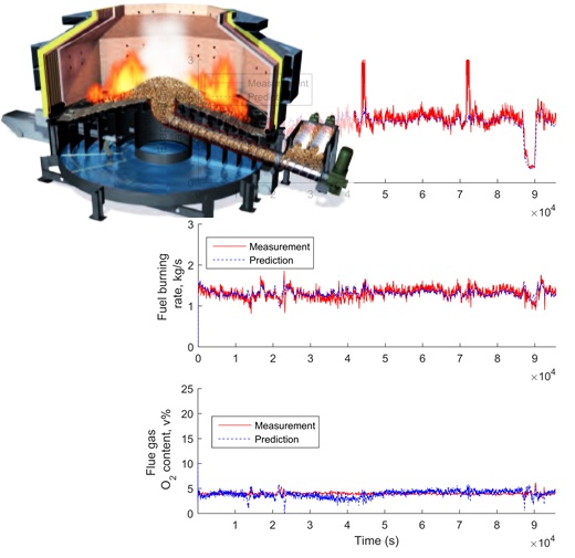
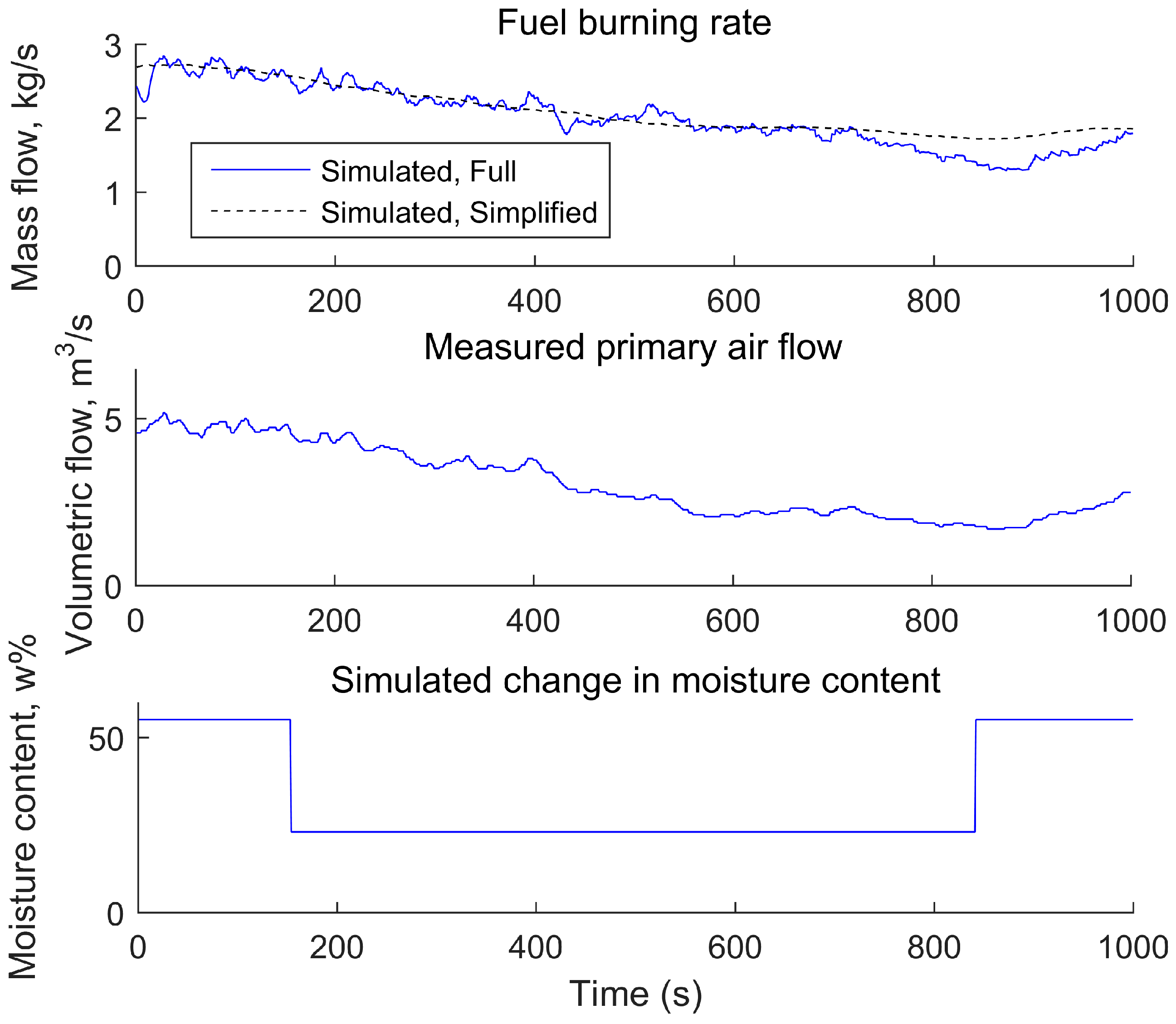
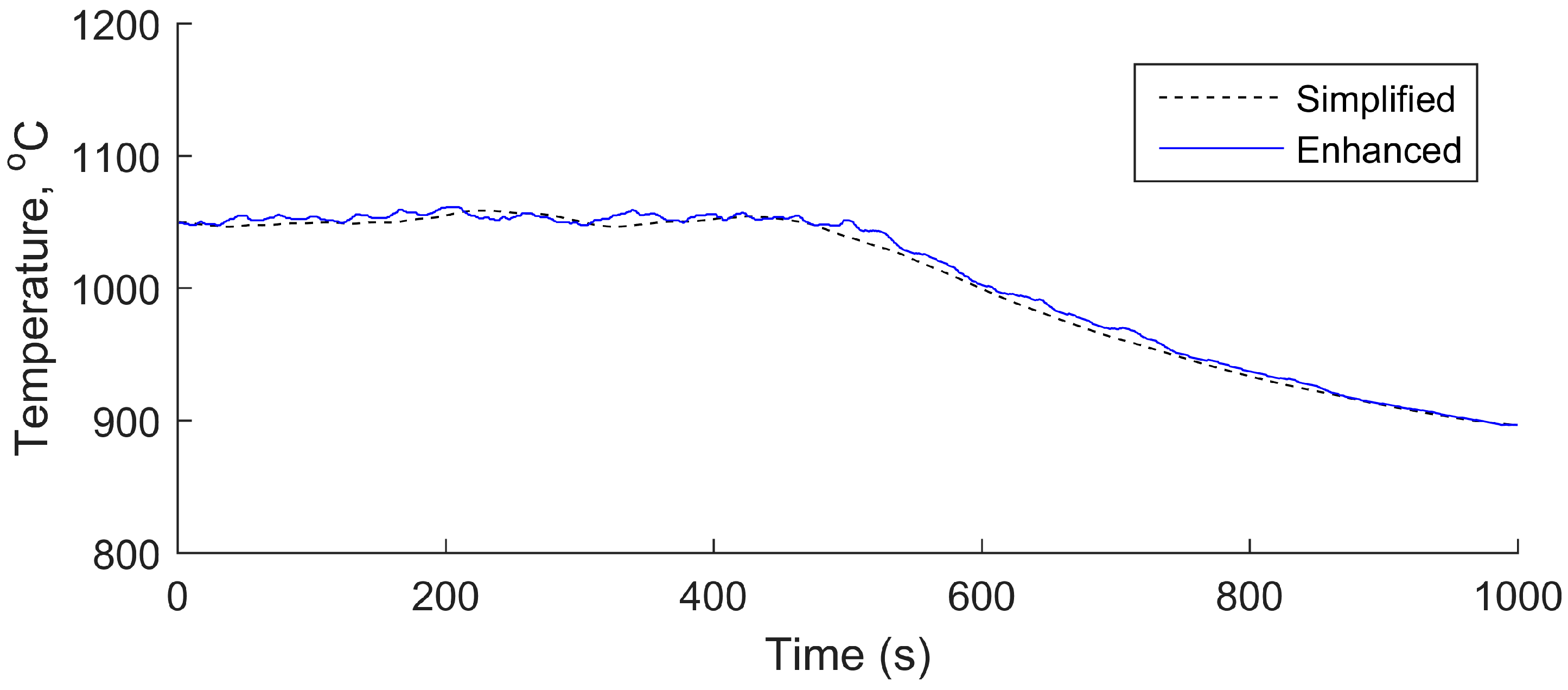
3.5. Simplified Model Validation with Industrial Data from a BioGrate Boiler

The objective of the model validation was to evaluate the model prediction of the combustion rate m_d and water evaporation rate m_w. Validation was performed against industrial data obtained during full-scale plant experiments at BioPower 5, 16 MW CHP, a BioGrate boiler located at Mänttä-Vilppula, Finland. The aim of the experiments was to study the effect of fuel moisture content variations on the boiler operations. For this purpose, three changes in the fuel moisture content were induced by switching the fuel feed to the auxiliary fuel bunker loaded with 5 m³, 10 m³ and 25 m³ wood chips with approximately 22 wt% moisture content. After the bunker contents were fully discharged, the fuel feed was switched back to the typical fuel, having 55 wt% moisture content. Thus, the experiment induced fast changes in the process operations, which are suitable to test the ability of the simplified model to describe combustion phenomena during rapid transitions in fuel quality.

During the experiments, the residual oxygen content, X_O2, was directly available from the database of the automation system. The values for the molar fraction of water vapor, X_H2O, were obtained with a Servomex 2500 FTIR Analyzer (Crowborough, UK) by probing the flue gas after the economizer. The data was collected with the one second sampling interval and then utilized for validation purposes along with the measured primary and secondary air flowrates and stoker speed.

The model prediction of the burning rates was calculated from the amount of consumed char and pyrolysis gas, while the evaporation rate was computed through the summation of evaporation rate due to convection and due to radiation, Equations (47) and (48), respectively. The combustion and evaporation rates predicted by the model were compared to the ones calculated from the experimental data which were obtained by solving Equations (60)–(65) for the evaporation rate, m_w, as well as the combustion rate, m_d:

$$X_{{\mathrm{O}}_2}=\frac{{\dot{n}}_{{\mathrm{O}}_2}}{{\dot{n}}_{{\mathrm{N}}_2}+{\dot{n}}_{{\mathrm{H}}_2\mathrm{O}}+{\dot{n}}_{{\mathrm{O}}_2}+{\dot{n}}_{{\mathrm{CO}}_2}}$$

(60)

$$X_{{\mathrm{H}}_2\mathrm{O}}=\frac{{\dot{n}}_{{\mathrm{H}}_2\mathrm{O}}}{{\dot{n}}_{{\mathrm{N}}_2}+{\dot{n}}_{{\mathrm{H}}_2\mathrm{O}}+{\dot{n}}_{{\mathrm{O}}_2}+{\dot{n}}_{{\mathrm{CO}}_2}}$$

(61)

where ${\dot{n}}_{{\mathrm{N}}_2}, {\dot{n}}_{{\mathrm{H}}_2\mathrm{O}}, {\dot{n}}_{{\mathrm{O}}_2} \text{and} {\dot{n}}_{{\mathrm{CO}}_2}$ are the molar contents of the components in the flue gas, and X_O2 and X_H2O are the volumetric fractions of oxygen and water vapor in flue gas. The molar composition of the flue gas is defined as follows:

$${\dot{n}}_{{\mathrm{O}}_2}=0.23\frac{{\dot{m}}_{\mathrm{Air}}}{M_{{\mathrm{O}}_2}}+\left(-\frac{0.51}{M_{\mathrm{C}}}-\frac{0.06}{2M_{{\mathrm{H}}_2}}+\frac{0.41}{M_{{\mathrm{O}}_2}}\right)\cdot {\dot{m}}_{\mathrm{d}}$$

(62)

$${\dot{n}}_{{\mathrm{H}}_2\mathrm{O}}=0.06\frac{{\dot{m}}_{\mathrm{d}}}{M_{{\mathrm{H}}_2}}+\frac{{\dot{m}}_{\mathrm{W}}}{M_{{\mathrm{H}}_2\mathrm{O}}}$$

(63)

$${\dot{n}}_{{\mathrm{CO}}_2}=0.51\frac{{\dot{m}}_{\mathrm{d}}}{M_{\mathrm{C}}}$$

(64)

$${\dot{n}}_{{\mathrm{N}}_2}=0.77\frac{{\dot{m}}_{\mathrm{Air}}}{M_{{\mathrm{N}}_2}}$$

(65)

where m_Air is the mass flow of the combined primary and secondary air, m_d is the combustion rate of fuel, and m_w is the evaporation rate of fuel moisture. M_H2, M_H2O, M_C, and M_N2 are the molar weights of hydrogen, water, carbon, and nitrogen, respectively.

The process inputs during the experiment, presented in Figure 5, were used as model inputs to obtain the model prediction of the process variables. The validation results presented in Figure 6 confirm a sufficient descriptive ability of the model. In particular, the variations in the air flows result in slightly lower fuel burning rate while dryer fuel is used, which is reproduced well by the simplified model. The amount of water in the fuel feed directly affects the evaporation rate, the dynamics of which follows closely the model prediction. Furthermore, only a minor difference can be observed between the model prediction for the oxygen content in the flue gas and its measured value, maintained at the constant level by the plant control system. In fact, the model prediction error for the flue gas oxygen is correlated with the prediction error of the burning rate. For example, the model slightly overestimates the burning rate between 30,000 s and 45,000 s of the simulation time, which results in overestimating the oxygen consumption and underestimating the oxygen content in the flue gas. This presents a possibility of utilizing the flue gas oxygen measurement for further improvement in the accuracy of the on-line predictions.

The dynamics of the model states, including the temperature of char and gas, as well as the amount of char, fuel and water on the grate, are presented in Figure 7. The predicted gas and burning char (solid) temperatures are in a good agreement with the values previously measured by Cooper and Hallett [28]. The variations in fuel moisture content result in large changes in char and gas temperature, as presented in Figure 7, which have a major impact on the rates of combustion reactions. Moreover, switching to a dryer fuel raises the amount of char on the grate and simultaneously decreases the quantity of fuel and moisture. Thus, the increased char to fuel ratio requires the adjustment of primary to secondary air ratio in order to achieve clean combustion.

Summarizing, the model demonstrated the ability to describe the fuel burning and evaporation rates that determine the power production of the boiler. Furthermore, the insight provided by the simplified model is especially attractive for the implementation of an efficient model-based process control the boiler. This efficiency can be achieved through the model-based estimation of the attainable power load transitions and load limits could be estimated to avoid the risk of combustion extinguishing or inefficient biomass firing. Thus, the validation results support the use of the simplified model for flexible control of power generation.

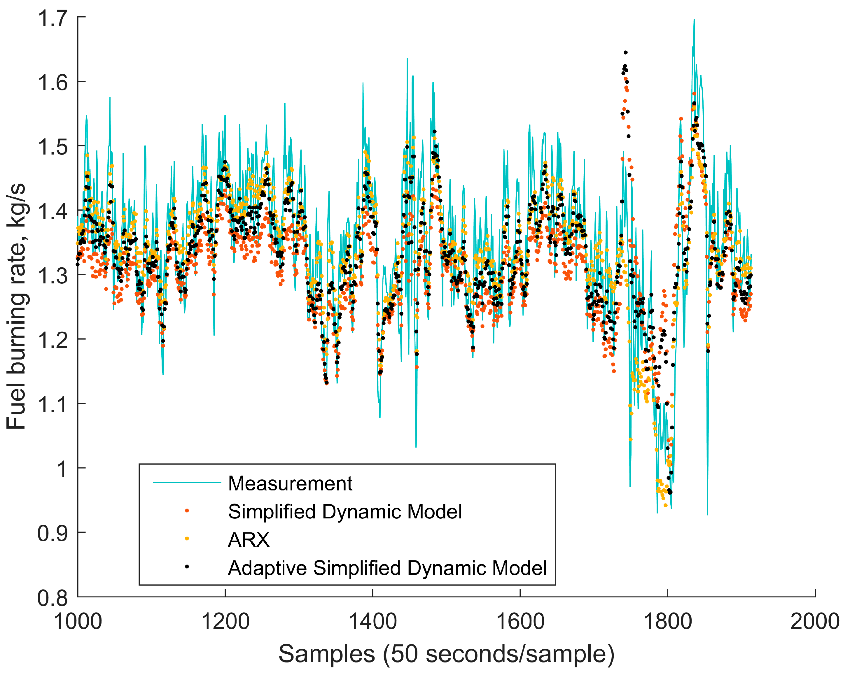
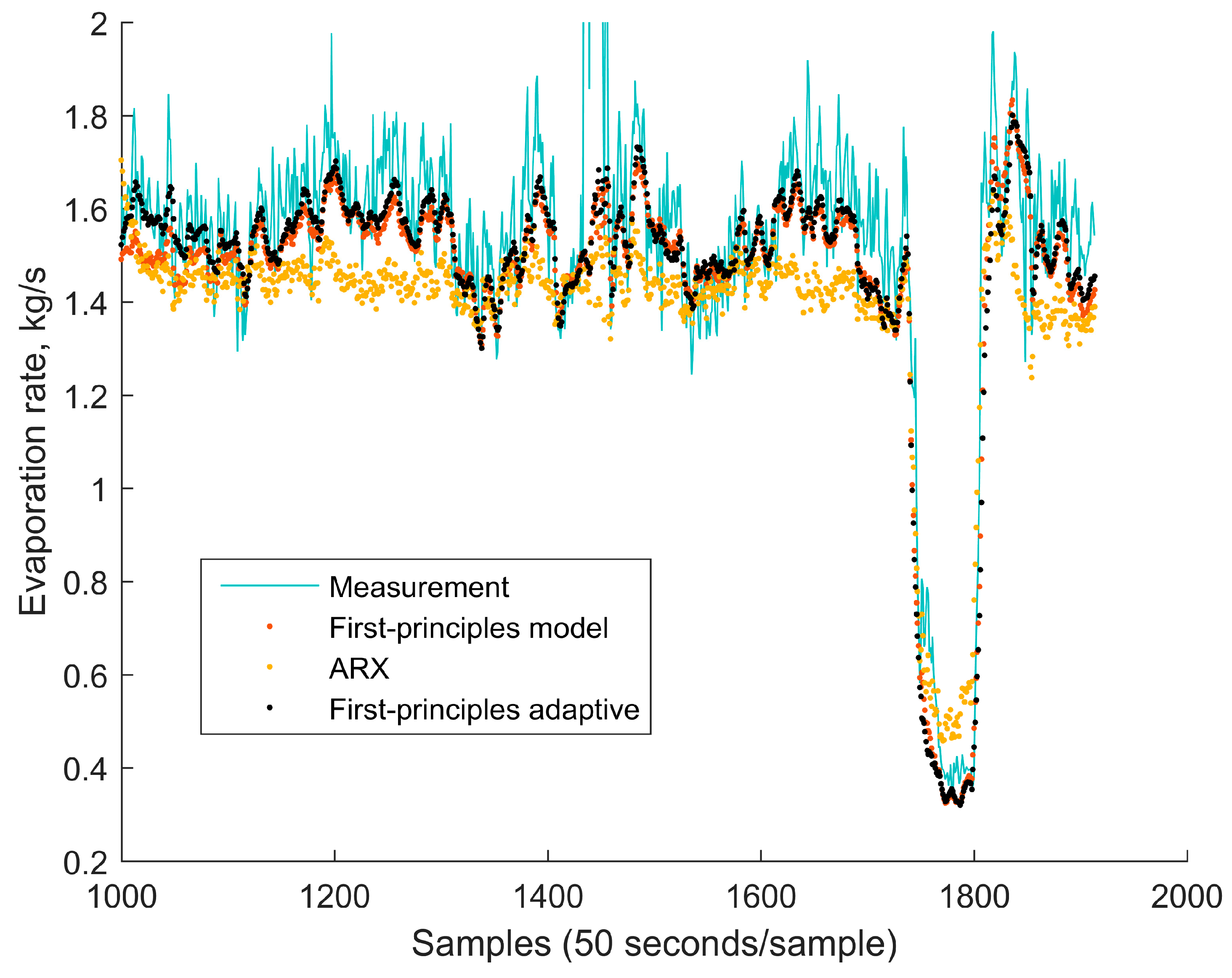
4. Performance Evaluation of the Simplified Model Predictions against the Predictions from the Mechanistic Model and Autoregressive Model with Exogenous Inputs

4.1. Comparison of the Simplified Dynamic Model against the Mechanistic Model

This section discusses the comparison of the results from the full-scale and the simplified models for a fuel moisture change scenario. In this scenario, the fuel moisture was switched from 55 wt% to 22 wt% at 160 s and back to 55 wt% at 840 s of the simulation time, as shown in Figure 8. The decreased primary air flow between 200 s and 800 s delivered less oxygen to the furnace for the combustion reactions. This reduced the burning rate, as predicted by both the full-scale and the simplified models, as demonstrated in Figure 8. In contrast, as the moisture content of the fuel is increased back to the initial level, the primary air flow and the burning rate rise to provide increased amount energy for the fuel drying. This is visible as an increase in the combustion rate in the period that occurred at the time instance of 800 s from the beginning of the simulation.

In general, both models predict similar burning rate trends, agreeing with the process knowledge. However, the prediction of the full-scale model is more sensitive to the high-frequency variations of the primary air flow, as confirmed by Figure 8. This is due to faster local temperature changes in the full model since in the simplified model the temperature is averaged over the whole char layer resulting in slower temperature variations. The temperatures of char layer from both models are presented in Figure 9, in case of the mechanistic model, the temperature was averaged over the char layer. The temperature of the char layer follows the primary air flow dynamics, namely, larger airflows result in larger temperatures while lower flow rate produces lower temperatures. The effect of convective cooling on char by the primary air has lower effect on the temperature compared to the effect of decreased combustion intensity, resulting in lower combustion temperatures at low flow rates.

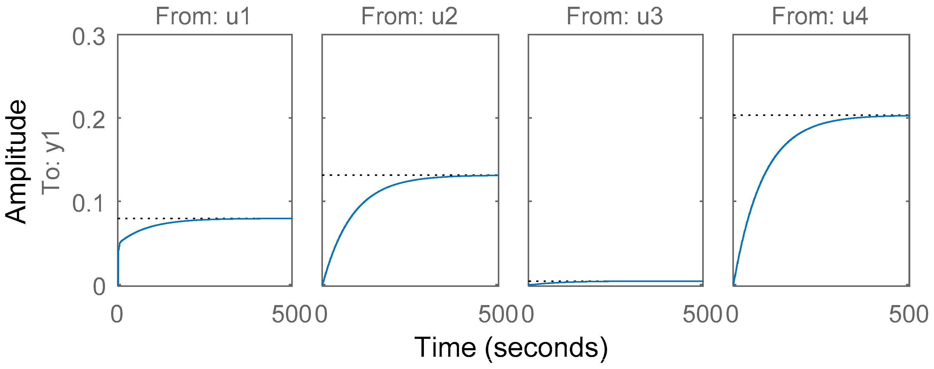
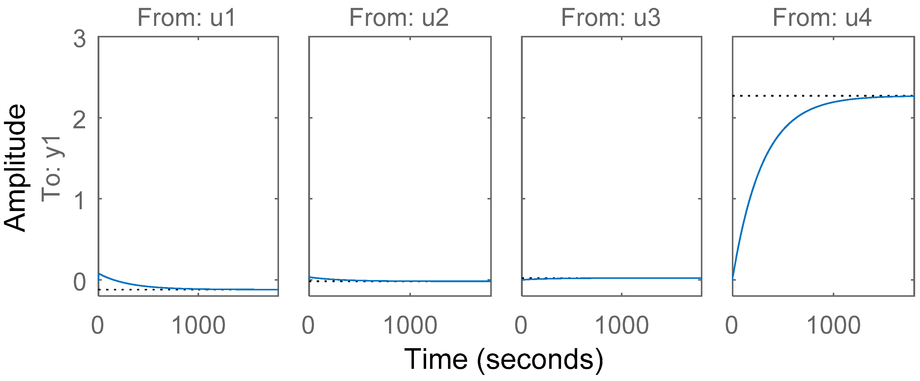
4.2. Comparison of the Simplified Dynamic Model against a Linear Autoregressive Model with Exogenous Inputs Model

In this section, the predictions from the simplified model are compared to the predictions from linear data based-model. The ARX model structure was selected for the linear data based-model due to its satisfactory ability in capturing process dynamics, fast identification and straightforward model diagnostics. The comparison allows the evaluation of the degree of the process nonlinearity effect on the accuracy of a linear model. For the comparison, two ARX models were identified from process data for the moisture evaporation and the fuel burning rates, respectively. The autocorrelation of the model residuals and its cross-correlation with the model inputs were evaluated to ensure the assumptions of the identification methods. Different model orders were tried, and fourth order delivered the best results in both cases.

The step responses are presented in Figure 10 for the identified burning-rate-ARX model and in Figure 11 for the evaporation model. For the burning rate ARX model, the secondary air has twice the effect on the combustion rate compared to the primary air, which seems to be unreasonably high. In fact, the secondary air could be more sensitive to the burning rate variations compared other process inputs because the process control adjusts the secondary air according to the oxygen consumption to maintain the flue gas oxygen constant. Furthermore, the stoker speed has negligible effect on the burning rate, because the stoker speed is coupled with the primary air flow rate in the control strategy of the boiler and the data-based modeling is unable to separate the effect of these two inputs on the process dynamics. However, the stoker speed essentially controls the amount of fuel on the grate and subsequently the combustion rate, thus contradicting the degree of the effect of stoker speed identified by the model. The significance of the moisture content on the combustion rate appears reasonable, although according to the model, the increase in moisture content increases burning rate which is in conflict with the process knowledge. The moisture content affects the ignition delay of the fuel rather than having a direct effect on the magnitude of the combustion rate.

For the second model, the step responses shown in Figure 11 indicated that only fuel moisture content has a significant effect on the evaporation rate, while other inputs have virtually no influence on the model output. This contradicts to the process knowledge, as the fuel feed rate, determined by the stoker speed, directly influences the amount of water delivered to the furnace, and therefore, certainly affects the evaporation rate. Furthermore, as increasing the primary airflow intensifies the burning rate and the amount of heat released, it should thereby increase the evaporation rate as well.

As discussed in Section 3.5, a correlation exists between the simplified model prediction errors of the flue gas oxygen content and the burning rate. Thus, an adaptive modification of the simplified model was developed correcting its estimation of the combustion coefficient in Equation (45) by means of a PI controller. In more detail, the coefficient is adjusted on-line as follows:

$$k_{\mathrm{pyr},\mathrm{comb}}=u(t)T_{\mathrm{gas}}/T_{\mathrm{char}}{k}_{\mathrm{C}}$$

(66)

where u(t) is the output signal of the PI controller:

$$u(t)=\max \left(\frac{5}{1000}\cdot \left(e(t)+\frac{1}{10}{\displaystyle \int e}(\mathsf{\tau })\hspace{0.17em}\mathrm{d}t\right),\hspace{0.17em}0\right)$$

(67)

receiving the flue gas oxygen prediction error defined by Equation (68):

$$e(t)=X_{{\mathrm{O}}_2,\mathrm{meas}}(t)-X_{{\mathrm{O}}_2,\mathrm{pred}}(t)$$

(68)

The comparison indicates that all three models: the simplified, simplified adaptive and data based-model are able to predict the fuel combustion rate due to a linear relation of fuel consumption to primary and secondary air flow during the experiment (Figure 12). The adaptive modification of the simplified model, utilizing the flue gas oxygen measurement to correct the burning rate prediction, provides a little more accurate results compared to the original simplified model. The results shown in Figure 12 confirm that the ARX model can be accurate in certain operating conditions, when the burning rate, not restricted by the amount of combustible materials available, depends linearly on the air flows. However, the adequacy of the ARX model at largely varying operating conditions and rapid transitions is questionable, as it is unable to monitor the amount of fuel and char in the furnace. This conclusion is confirmed by the step responses shown in Figure 10, not fully agreeing with the process knowledge.

The evaporation rate, presented in Figure 13, was predicted sufficiently well only by the simplified dynamic models. ARX model demonstrated only a minor ability to follow the variations observed in the evaporation rate. One explanation to the observed ARX model deficiency is that drying depends on nonlinear factors such as heat radiation from oxidation zone and to properly account for these factors, a nonlinear model is required for a proper description of combustion phenomena.

4.3. Comparison of Computational Times of Different Models

The models—including the mechanistic model, simplified model and ARX models—were compared in terms of their run times and the results are presented in

Table 2. Run times of different models on different computer configurations.

Computer	Mechanistic (Real-Time Seconds/Simulated Second)	Simplified	ARX
Laptop	14.173497	6.23 × 10−4	7.21 × 10−7
Desktop-1 (R2014b)	5.403695	5.34 × 10−4	6.477 × 10−7
Desktop-1 (R2015b)	31.443311	2.81 × 10−4	7.066 × 10−7
Desktop-2	28.240536	2.11 × 10−4	5.927 × 10−7

while the associated computer configurations are shown in

Table 3. Computer configurations.

Computer	Matlab Version	RAM (GB)	CPU Model	Frequency (GHz)	# of Cores	# of Threads
Laptop	R2015a	8	Intel i5-3340M	2.7	2	4
Desktop-1	R2014b	12	Intel i7 920	3.6	4	8
Desktop-2	R2015b	8	Intel Xeon E3-1230	3.2	4	8

. The computational times of the mechanistic model largely benefit from the parallel computations in Matlab versions below R2015b and both clock frequency and the number of CPU cores. A larger number of processor cores and higher clock frequencies allowed Desktop-1 to perform almost three times faster compared to the laptop computer. On these two computers, computational times of ARX and the simplified model benefitted less from a larger core number and higher clock frequencies. Matlab version R2015b demonstrated significantly longer computational times for the mechanistic model and were almost six times longer when compared to the simulation time obtained on computer Desktop-1 running R2014b, possibly due to some deficiencies in the parallel computing toolbox. Nevertheless, the computational times of the simplified model on the newer Matlab version on Desktop-1 were almost two times faster than on Desktop-1 running an older version. Furthermore, the Desktop-2 demonstrated even further improvements in computational times due to the upgrades in the CPU architecture and these advancements resulted in faster computational times of the ARX model.

5. Conclusions

In this work, a mechanistic biomass combustion model developed for process phenomena investigation was simplified to obtain a model describing the combustion phenomena and suitable for applications requiring fast computational time. The simplified model was validated with industrial data from the process and demonstrated sufficient accuracy in describing the combustion of biomass fuel. The adaptive modification introduced to the simplified model provided further improvement of the burning and evaporation rates prediction.

Increasing demand for power production flexibility and handling the unmeasured variations of fuel properties require advanced process control techniques, such as model predictive control. Based on an underlying model able to describe the combustion phenomena, this control technique would allow one to avoid fuel burnout and to prevent incomplete fuel combustion and formation of pollutants in the furnace. As was demonstrated by the results, the deep insight into the process conditions provided by the model allows to ensure that prerequisites for a fast load transition, such as sufficient amount of fuel in the furnace. Furthermore, the power production flexibility can be supported through on-line monitoring of the furnace state, including fuel amount and composition, temperature as well as the composition of the forming flue gas. In contrast, as was demonstrated in this article, the models identified from process data fail to capture the key relations between the variables which cause performance deficiencies if utilized for process control. In this work, the simplified model of the biomass combustion is obtained for control and monitoring algorithms implementation, whereas its low computational load allows its utilization in on-line calculations.

References

1. Hogg, B.; El-Rabaie, N. Multivariable generalized predictive control of a boiler system. IEEE Trans. Energy Convers. 1991, 6, 282–288. [Google Scholar] [CrossRef]
2. Bauer, R.; Gölles, M.; Brunner, T.; Dourdoumas, N.; Obernberger, I. Modelling of grate combustion in a medium scale biomass furnace for control purposes. Biomass Bioenergy 2010, 34, 417–427. [Google Scholar] [CrossRef]
3. Gölles, M.; Reiter, S.; Brunner, T.; Dourdoumas, N.; Obernberger, I. Model based control of a small-scale biomass boiler. Control Eng. Pract. 2014, 22, 94–102. [Google Scholar] [CrossRef]
4. Kortela, J.; Jämsä-Jounela, S. Model predictive control utilizing fuel and moisture soft-sensors for the BioPower 5 combined heat and power (CHP) plant. Appl. Energy 2014, 131, 189–200. [Google Scholar] [CrossRef]
5. Flynn, M.; O’Malley, M. A drum boiler model for long term power system dynamic simulation. IEEE Trans. Power Syst. 1999, 14, 209–217. [Google Scholar] [CrossRef]
6. Paces, N.; Kozek, M. Modeling of a Grate-Firing Biomass Furnace for Real-Time Application. In Proceedings of the International Symposium on Qualitative, Quatitative and Hybrid Models and Modeling Methodologies in Science and Engineering (MMMse 2011), Orlando, FL, USA, 27–30 March 2011.
7. Belkhir, F.; Meiers, J.; Felgner, F.; Frey, G. A Biomass Combustion Plant Model for Optimal Control Applications—The Effect of Key Variables on Combustion Dynamics. In Proceedings of the 6th International Renewable Energy Congress (IREC), Sousse, Tunisia, 24–26 March 2015; pp. 1–6.
8. Liu, X.; Kong, X.; Hou, G.; Wang, J. Modeling of a 1000 MW power plant ultra super-critical boiler system using fuzzy-neural network methods. Energy Convers. Manag. 2013, 65, 518–527. [Google Scholar] [CrossRef]
9. Peng, H.; Nakano, K.; Shioya, H. Nonlinear predictive control using neural nets-based local linearization ARX model—Stability and industrial application. IEEE Trans. Control Syst. Technol. 2007, 15, 130–143. [Google Scholar] [CrossRef]
10. Havlena, V.; Findejs, J. Application of model predictive control to advanced combustion control. Control Eng. Pract. 2005, 13, 671–680. [Google Scholar] [CrossRef]
11. Leskens, M.; Van Kessel, L.; Van den Hof, P. MIMO closed-loop identification of an MSW incinerator. Control Eng. Pract. 2002, 10, 315–326. [Google Scholar] [CrossRef]
12. Leskens, M.; Van Kessel, L.; Bosgra, O. Model predictive control as a tool for improving the process operation of MSW combustion plants. Waste Manag. 2005, 25, 788–798. [Google Scholar] [CrossRef] [PubMed]
13. Morari, M.; Lee, J.H. Model predictive control: Past, present and future. Comput. Chem. Eng. 1999, 23, 667–682. [Google Scholar] [CrossRef]
14. Boriouchkine, A.; Zakharov, A.; Jämsä-Jounela, S. Dynamic modeling of combustion in a BioGrate furnace: The effect of operation parameters on biomass firing. Chem. Eng. Sci. 2012, 69, 669–678. [Google Scholar] [CrossRef]
15. Boriouchkine, A.; Sharifi, V.; Swithenbank, J.; Jämsä-Jounela, S. A study on the dynamic combustion behavior of a biomass fuel bed. Fuel 2014, 135, 468–481. [Google Scholar] [CrossRef]
16. Pomerantsev, V. Fundamentals of Applied Combustion Theory; Energoatomizdat: Moscow, Russia, 1986. [Google Scholar]
17. Fogler, S. Elements of Chemical Reaction Engineering, 4th ed.; Pearson Educations: Upper Saddle River, NJ, USA, 2006. [Google Scholar]
18. Branca, C.; Di Blasi, C. Devolatilization and combustion kinetics of wood chars. Energy Fuels 2003, 17, 1609–1615. [Google Scholar] [CrossRef]
19. Senneca, O. Kinetics of pyrolysis, combustion and gasification of three biomass fuels. Fuel Process. Technol. 2007, 88, 87–97. [Google Scholar] [CrossRef]
20. Matsumoto, K.; Takeno, K.; Ichinose, T.; Ogi, T.; Nakanishi, M. Gasification reaction kinetics on biomass char obtained as a by-product of gasification in an entrained-flow gasifier with steam and oxygen at 900–1000 °C. Fuel 2009, 88, 519–527. [Google Scholar] [CrossRef]
21. Evans, D.D.; Emmons, H. Combustion of wood charcoal. Fire Saf. J. 1977, 1, 57–66. [Google Scholar] [CrossRef]
22. Janssens, M.; Douglas, B. Wood and Wood Products. In Handbook of Building Materials for Fire Protection; Harper, C.A., Ed.; McGraw-Hill: New York, NY, USA, 2004. [Google Scholar]
23. Shin, D.; Choi, S. The combustion of simulated waste particles in a fixed bed. Combust. Flame 2000, 121, 167–180. [Google Scholar] [CrossRef]
24. Branca, C.; Blasi, C.D.; Elefante, R. Devolatilization and heterogeneous combustion of wood fast pyrolysis oils. Ind. Eng. Chem. Res. 2005, 44, 799–810. [Google Scholar] [CrossRef]
25. Boriouchkine, A.; Sharifi, V.; Swithenbank, J.; Jämsä-Jounela, S. Experiments and modeling of fixed-bed debarking residue pyrolysis: The effect of fuel bed properties on product yields. Chem. Eng. Sci. 2015, 138, 581–591. [Google Scholar] [CrossRef]
26. Garcìa-Pérez, M.; Chaala, A.; Pakdel, H.; Kretschmer, D.; Roy, C. Vacuum pyrolysis of softwood and hardwood biomass: Comparison between product yields and bio-oil properties. J. Anal. Appl. Pyrolysis 2007, 78, 104–116. [Google Scholar] [CrossRef]
27. Wakao, N.; Kaguei, S.; Funazkri, T. Effect of fluid dispersion coefficients on particle-to-fluid heat transfer coefficients in packed beds: Correlation of nusselt numbers. Chem. Eng. Sci. 1979, 34, 325–336. [Google Scholar] [CrossRef]
28. Cooper, J.; Hallett, W.L.H. A numerical model for packed-bed combustion of char particles. Chem. Eng. Sci. 2000, 55, 4451–4460. [Google Scholar] [CrossRef]
Figure 1. BioGrate boiler furnace.
Energies 09 00735 g001
Figure 2. Outline of the model used for process phenomena investigation.
Energies 09 00735 g002
Figure 3. Overview of the model structure.
Energies 09 00735 g003
Figure 4. Simulation results from the enhanced model.
Energies 09 00735 g004
Figure 5. Inputs: fuel feed, fuel moisture, primary air, secondary air.
Energies 09 00735 g005
Figure 6. Measured and predicted outputs: moisture evaporation rate, fuel burning rate and flue gas content.
Energies 09 00735 g006
Figure 7. Model states during the validation: (a) char and gas temperatures, (b) amount of char, and (c) fuel and moisture content.
Energies 09 00735 g007
Figure 8. Comparison of the predictions from mechanistic to the ones from the simplified model.
Energies 09 00735 g008
Figure 9. Comparison of the predictions of averaged char layer temperatures from the mechanistic to the ones from the simplified model.
Energies 09 00735 g009
Figure 10. Step responses of the autoregressive model with exogenous inputs (ARX) model for burning rate prediction. u1: primary air; u2: secondary air; u3: stoker speed; and u4: fuel moisture content.
Energies 09 00735 g010
Figure 11. Step responses of the ARX model for evaporation rate prediction. u1: primary air; u2: secondary air; u3: stoker speed; and u4: fuel moisture content.
Energies 09 00735 g011
Figure 12. Comparison of burning rates predicted by the simplified dynamic model, ARX, and the adaptive simplified dynamic model.
Energies 09 00735 g012
Figure 13. Comparison of evaporation rates predicted by the simplified dynamic model, ARX, and the adaptive simplified dynamic model.
Energies 09 00735 g013