
Optimal Electric and Heat Energy Management of Multi-Microgrids with Sequentially-Coordinated Operations


Abstract
:1. Introduction
2. Proposed Optimal Electric and Heat Energy Management of Cooperative Multi-Microgrids
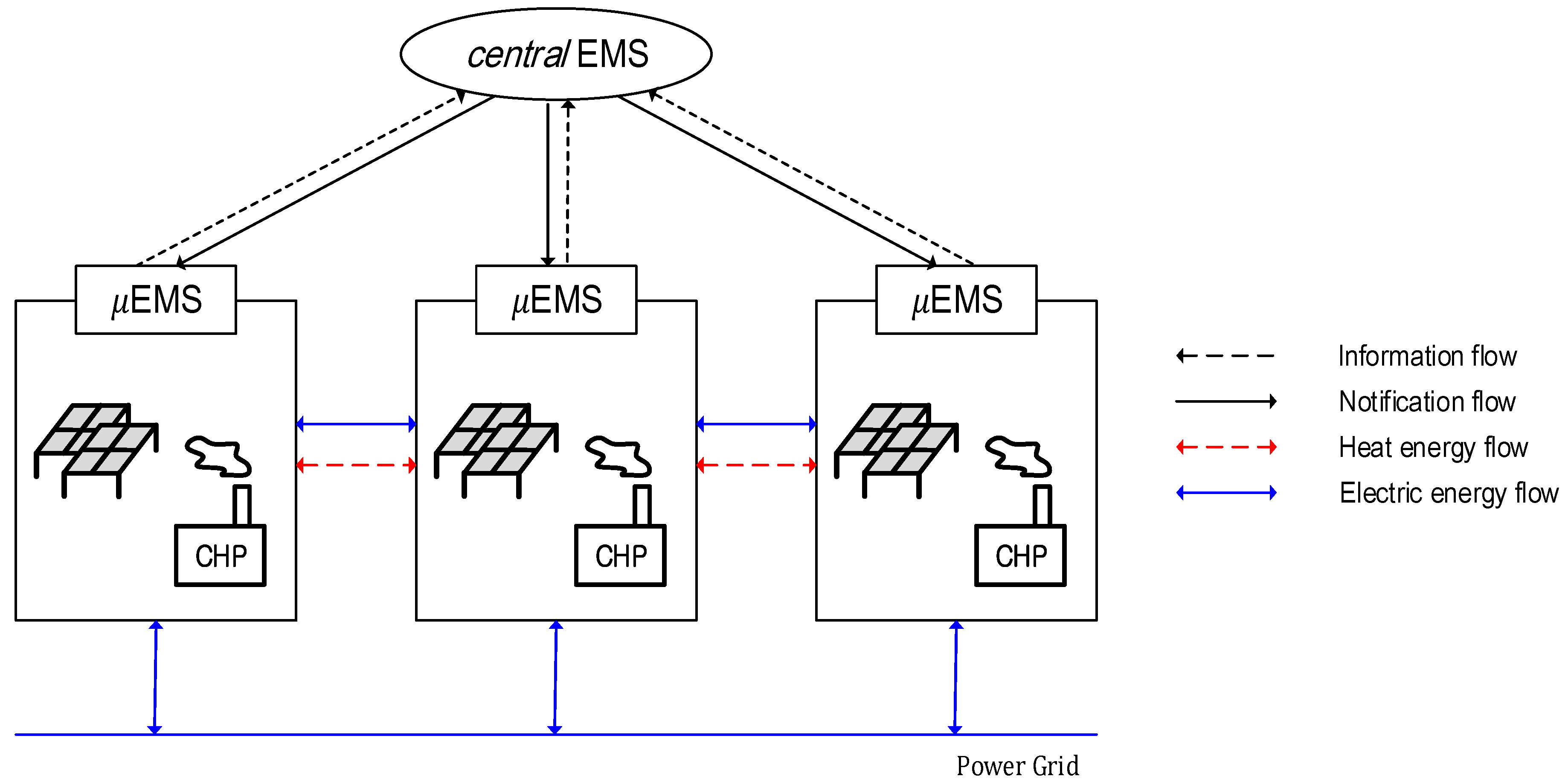
2.1. Cooperative Multi-Microgrid Community
- microgrids are equipped with photovoltaic (PV) systems, CHP generators, HOBs, and solar heat systems, but the production costs of CHP generators are different;
- microgrids can trade electric energy not only internally with other microgrids in the cooperative community but also externally with the power grid;
- microgrids allow only internal trading for heat energy with other microgrids in the cooperative community; this means that all heat loads should be self-supplemented by heat energy sources in the cooperative multi-microgrid community;
- a microgrid energy management system (μEMS) manages electric energy of its microgrid; and
- a central energy management system (central EMS) has a global optimization function to manage energy generators in multi-microgrids and to satisfy both electric and heat energy loads demanded by all multi-microgrids in the cooperative community.
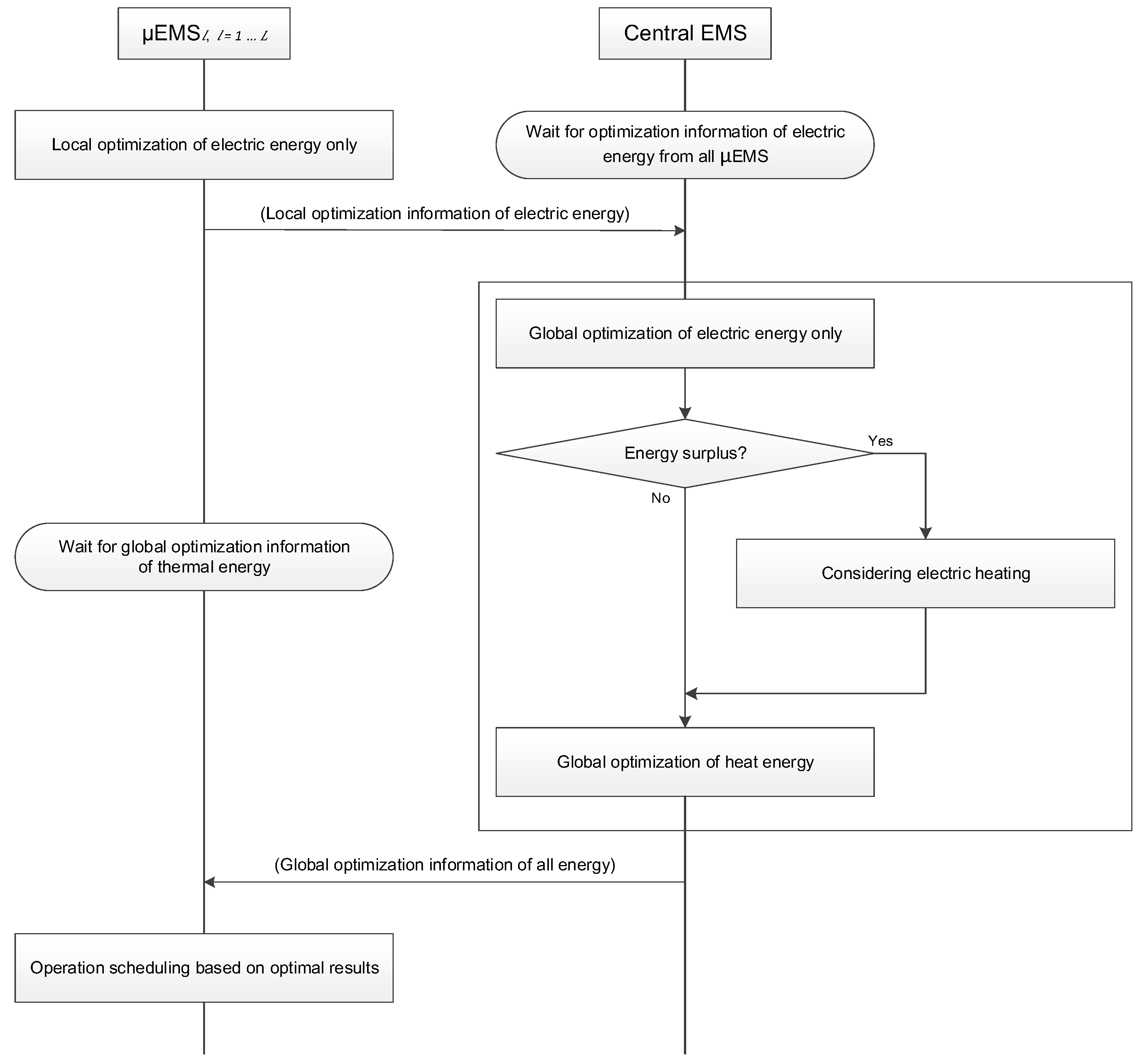
2.2. Operation Process of Cooperative Multi-Microgrids
- Step E-1: Local optimization of electric energy in each microgrid by the μEMS;
- Step E-2: Global electric energy trading optimization by the central EMS;
- Step H: Global heat energy optimization by the central EMS.
3. Mathematical Modeling of Cooperative Multi-Microgrid Operation for Electric Energy [9]
3.1. Nomenclature
- ₩ = South Korea Won
- = the identifier of operation interval
- = the number of operation intervals
- = the identifier of microgrid
- = the number of microgrid
- = the identifier of HOB
- = the number of HOBs
- = the identifier of electric energy
- = the electric energy production cost of the CHP in the microgrid (won/kWh)
- = the buying price from the power grid in the microgrid at (won /kWh)
- = the selling price to the power grid in the microgrid at (won /kWh)
- = the heat energy production cost of the CHP in the microgrid (won /kWh)
- = the cost of the HOB in the microgrid (won /kWh)
- = electric energy demand in the microgrid at (kWh)
- = the amount of surplus electric energy in the microgrid at (kWh)
- = the amount of short electric energy in the microgrid at (kWh)
- = the output produced from the PV system in the microgrid at (kWh)
- = the electric energy production amount of the CHP in the microgrid at (kWh)
- = the increased electric energy production amount of the CHP in the microgrid at (kWh) for the ancillary internal trading
- = the decreased electric energy production amount of the CHP in the microgrid at (kWh) for the ancillary internal trading
- = the amount of the buying electric energy in the microgrid determined by central EMS at (kWh)
- = the amount of the selling electric energy in the microgrid determined by central EMS at (kWh)
- = the received electric energy amount in the microgrid at (kWh)
- = the sending electric energy amount in the microgrid at (kWh)
3.2. Step E-1: Local Optimization of Electric Energy Operation Process
3.3. Step E-2: Global Optimization of Electric Energy Operation Process
4. Mathematical Modeling of Cooperative Multi-Microgrid Operation for Heat Energy
4.1. Nomenclature
- = the identifier of heat energy
- = the heat to power ratio of CHP in the microgrid (%)
- = heat energy demand in the microgrid at (kWh)
- = the amount of surplus heat energy in the microgrid at (kWh)
- = the amount of short heat energy in the microgrid at (kWh)
- = the output produced from the solar heat system in the microgrid at (kWh)
- = the heat energy production amount of the CHP in the microgrid at (kWh)
- = the additional heat energy amount of the CHP in the microgrid at (kWh)
- = the reducing heat energy amount of the CHP in the microgrid at (kWh)
- = the capacity of the CHP in the microgrid (kWh)
- = the received heat energy amount in the microgrid at (kWh)
- = the sending heat energy amount in the microgrid at (kWh)
- = the heat energy production amount of the HOB in the microgrid at (kWh)
- = the capacity of the HOB in the microgrid (kWh)
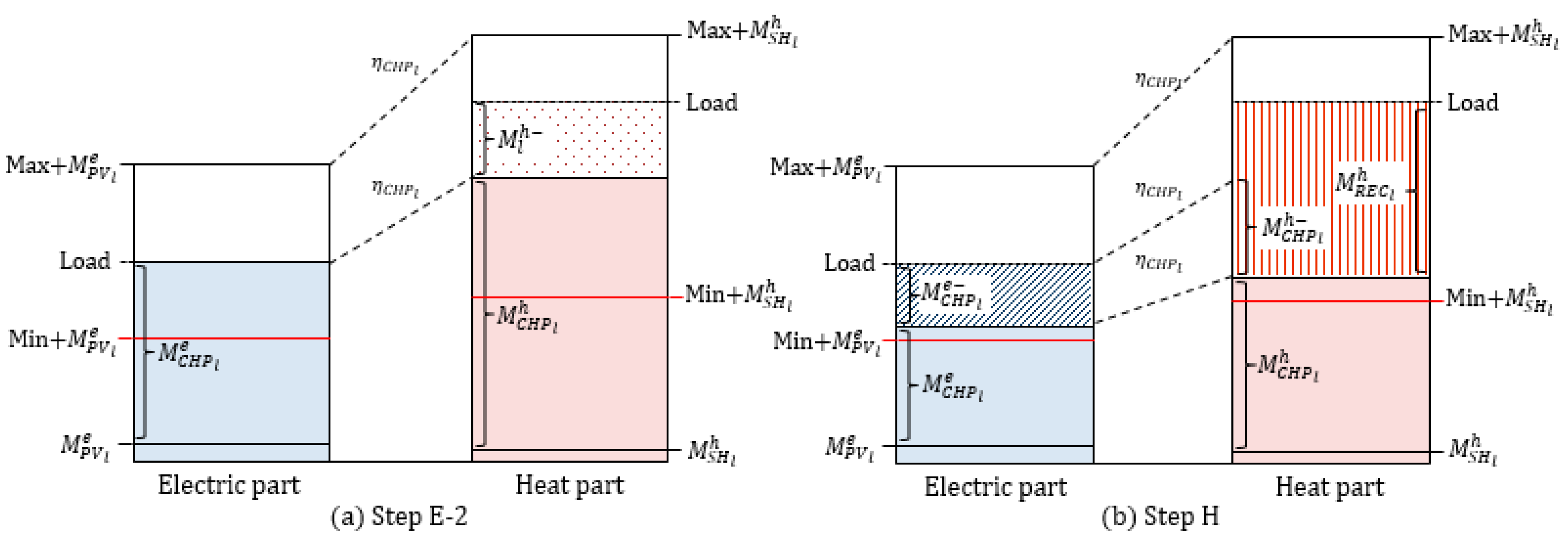
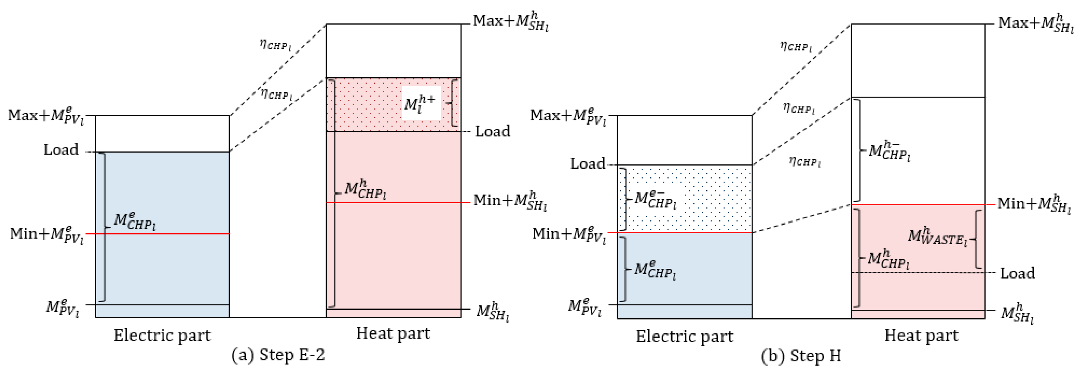
4.2. Step H: Mathematical Model of Global Heat Energy Optimization
4.3. Total Operation Costs
5. Simulation Study
6. Conclusions
Acknowledgments
Author Contributions
Conflicts of Interest
Appendix A. Linearization of the Adjusted Cost Function in Step H
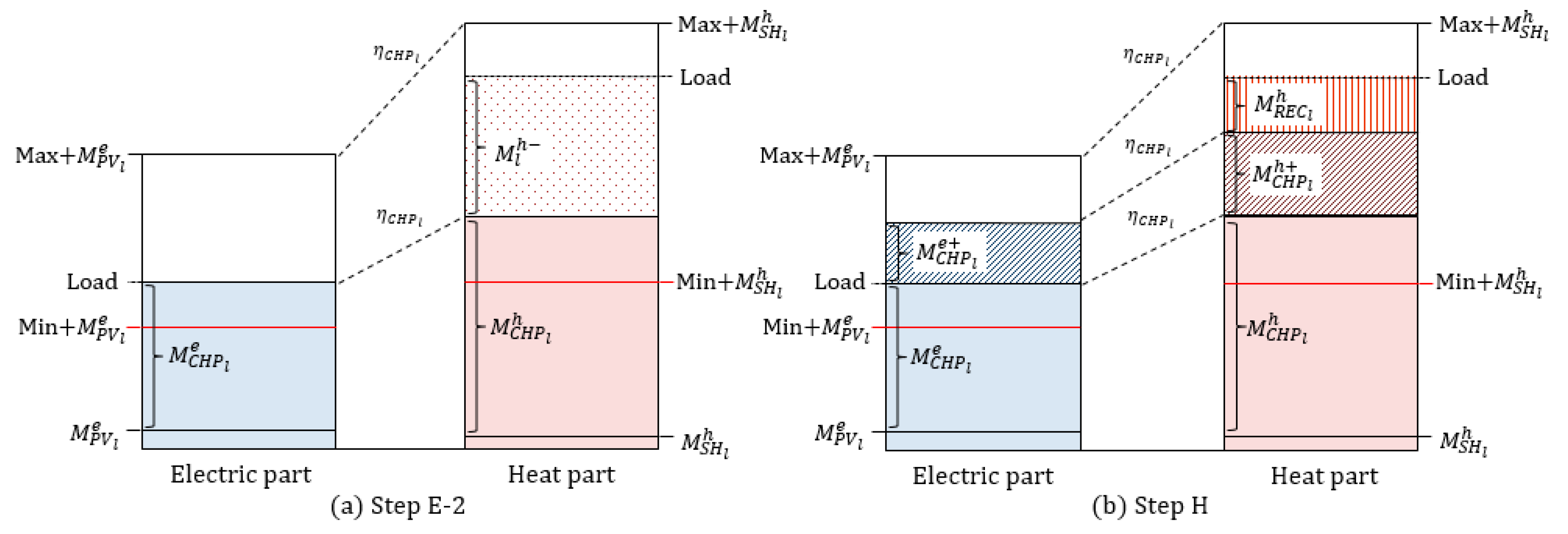
Appendix B. Illustrated Interpretation of Optimization Operation for Heat Energy


References
- Marnay, C.; Bailey, O. The CERTS microgrid and the future of the macrogrid. In Proceedings of the 2004 ACEEE Summer Study on Energy Efficiency in Buildings, Pacific Grove, CA, USA, 22–27 August 2004.
- Wood, E. The Importance of Heat in the Energy Efficient Microgrid. Available online: http://www.microgridknowledge.com/importance-heat-energy-efficient-microgrid/ (accessed on 23 January 2016).
- Kim, H.-M.; Kinoshita, T.; Shin, M.-C. A multiagent system for autonomous operation of islanded microgrids based on a power market environment. Energies 2010, 3, 1972–1990. [Google Scholar] [CrossRef]
- Lim, Y.; Kim, H.-M.; Kinoshita, T. Distributed load-shedding system for agent-based autonomous microgrid operations. Energies 2014, 7, 385–401. [Google Scholar] [CrossRef]
- Kim, H.-M.; Lim, Y.; Kinoshita, T. An intelligent multiagent system for autonomous microgrid operation. Energies 2012, 5, 3347–3362. [Google Scholar] [CrossRef]
- Yoo, C.-H.; Chung, I.-Y.; Lee, H.-J.; Hong, S.-S. Intelligent control of battery energy storage for multi-agent based microgrid energy management. Energies 2013, 6, 4956–4979. [Google Scholar] [CrossRef]
- Kuo, M.-T.; Lu, S.-D. Design and implementation of real-time intelligent control and structure based on multi-agent systems in microgrids. Energies 2013, 6, 6045–6059. [Google Scholar] [CrossRef]
- Vasiljevska, J.; Peças Lopes, J.A.; Matos, M.A. Multi-microgrid impact assessment using multi criteria decision aid methods. In Proceedings of the IEEE Bucharest 2009 PowerTech, Bucharest, Romania, 28 June–2 July 2009; pp. 1–8.
- Song, N.-O.; Lee, J.-H.; Kim, H.-M.; Im, Y.-H.; Lee, J.-Y. Optimal energy management of multi-microgrids with sequentially coordinated operations. Energies 2015, 8, 8371–8390. [Google Scholar] [CrossRef]
- Nguyen, T.A.; Mariesa, L.C. Optimization in energy and power management for renewable-diesel microgrids using dynamic programming algorithm. In Proceedings of the 2012 IEEE International Conference on Cyber Technology in Automation, Control, and Intelligent Systems (CYBER), Bangkok, Thailand, 27–31 May 2012; pp. 11–16.
- Khodaei, A. Resiliency-oriented microgrid optimal scheduling. IEEE Trans. Smart Grid 2014, 5, 1584–1591. [Google Scholar] [CrossRef]
- Chakraborty, S.; Simoes, M.G. PV-microgrid operational cost minimization by neural forecasting and heuristic optimization. In Proceedings of the 2008 IEEE Industry Applications Society Annual Meeting (IAS), Edmonton, AB, Canada, 5–9 October 2008; pp. 1–8.
- Chen, S.; Shroff, N.B.; Sinha, P. Energy trading in the smart grid: From end-user’s perspective. In Proceedings of the 2013 Asilomar Conference on Signals, Systems and Computers, Pacific Grove, CA, USA, 3–6 November 2013; pp. 327–331.
- Igualada, L.; Corchero, C.; Cruz-Zambrano, M.; Heredia, F.-J. Optimal energy management for a residential microgrid including a vehicle-to-grid system. IEEE Trans. Smart Grid 2014, 5, 2163–2172. [Google Scholar] [CrossRef]
- Chen, C.; Duan, S.; Cai, T.; Liu, B.; Yin, J. Energy trading model for optimal microgrid scheduling based on genetic algorithm. In Proceedings of the IEEE International Power Electronics and Motion Control 2009, Wuhan, China, 17–20 May 2009.
- Zhao, B.; Shi, Y.; Dong, X.; Laun, W.; Bornemann, J. Short-term operation scheduling in renewable-powered microgrids: A duality-based approach. IEEE Trans. Sustain. Energy 2014, 5, 209–217. [Google Scholar] [CrossRef]
- Ou, X.; Shen, Y.; Zeng, Z.; Zhang, G.; Wang, L. Cost minimization online energy management for microgrids with power and thermal storages. In Proceedings of the 24th International Conference on Computer Communication and Networks (ICCCN) 2015, Las Vegas, NV, USA, 3–6 August 2015.
- Bagherial, A.; Tafreshi, S.M.M. A developed energy management system for a microgrid in the competitive electricity market. In Proceedings of the IEEE PowerTech 2009, Bucharest, Romania, 28 June–2 July 2009.
- Nguyen, H.T.; Le, L.B. Optimal energy management for building microgrid with constrained renewable energy utilization. In Proceedings of the IEEE International Conference on Smart Grid Communications 2014, Venice, Italy, 3–6 November 2014.
- Chen, Y.-H.; Chen, Y.-H.; Hu, M.-C. Optimal energy management of microgrid systems in Taiwan. In Proceedings of the 2011 IEEE PES Innovative Smart Grid Technologies (ISGT), Hilton Anaheim, CA, USA, 17–19 January 2011; pp. 1–9.
- Kriett, P.O.; Salani, M. Optimal control of a residential microgrid. Energy 2012, 42, 321–330. [Google Scholar] [CrossRef]
- Rahbar, K.; Chai, C.C.; Zhang, R. Real-time energy management for cooperative microgrids with renewable energy integration. In Proceedings of the IEEE International Conference on Smart Grid Communications 2014, Venice, Italy, 3–6 November 2014.
- Nguyen, D.T.; Le, L.B. Optimal energy management for cooperative microgrids with renewable energy resources. In Proceedings of the 2013 IEEE International Conference on Smart Grid Communications, Vancouver, BC, Canada, 21–24 October 2013; pp. 678–683.


| Characteristics | CHP A | CHP B | CHP C |
|---|---|---|---|
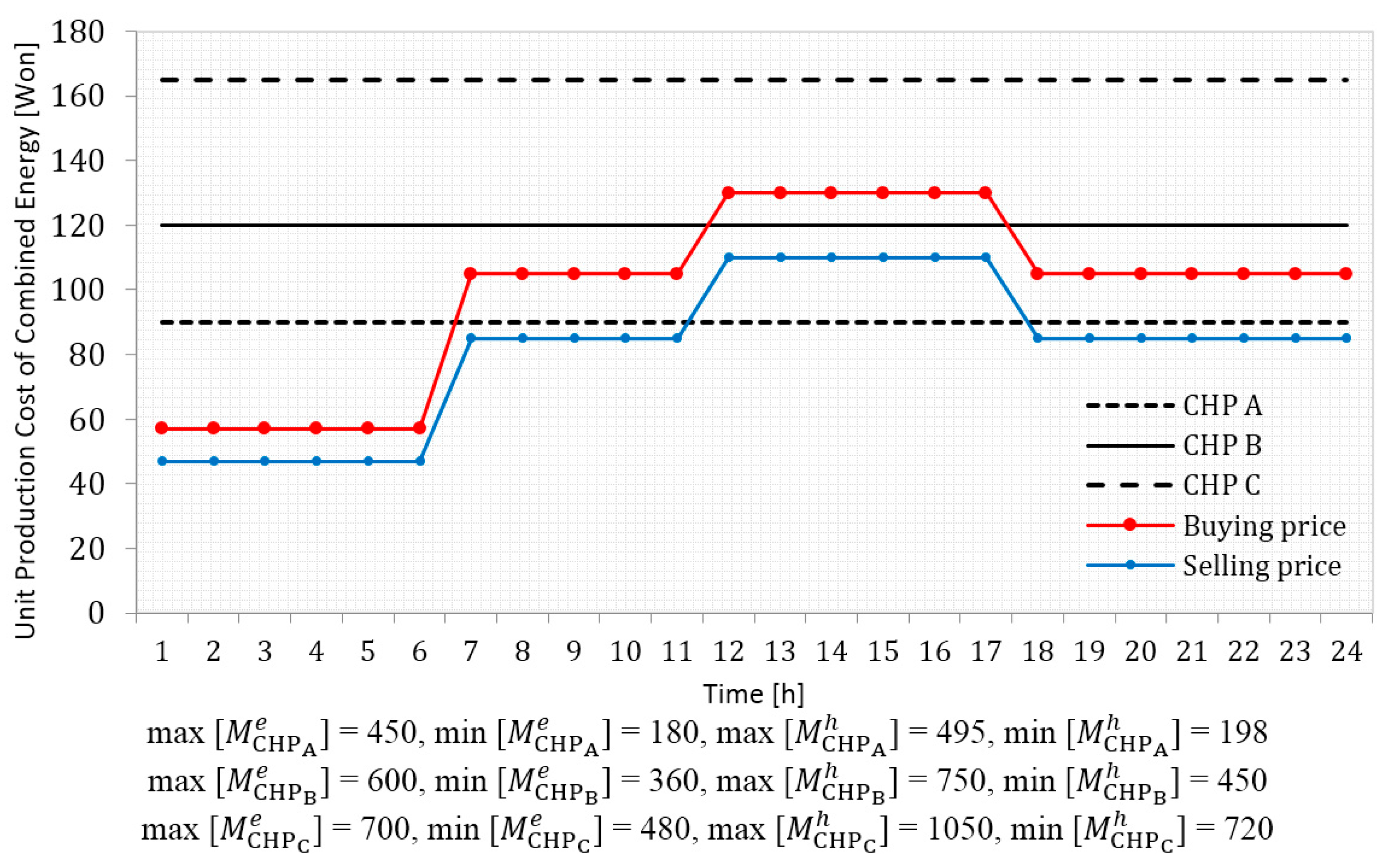
| Combined electric and heat (E and H) energy | 90 | 120 | 165 |
| 1 kWh Electric energy ( | 42.86 | 53.33 | 66 |
| kWh Heat energy ( | 47.14 | 66.67 | 99 |
| Heat and power ratio ( | 1.1 | 1.25 | 1.5 |
| Price | Off-Peak | Non-Peak | Peak |
|---|---|---|---|
| Buying price | 57 | 105 | 130 |
| Selling price | 47 | 85 | 110 |
| T | Microgrid A | Microgrid B | Microgrid C | ||||||||||||
|---|---|---|---|---|---|---|---|---|---|---|---|---|---|---|---|
| 1 | 369 | 450 | 0 | 0 | 81 | 192 | 360 | 0 | 0 | 168 | 550 | 480 | 0 | 70 | 0 |
| 2 | 345 | 450 | 0 | 0 | 105 | 187 | 360 | 0 | 0 | 173 | 525 | 480 | 0 | 45 | 0 |
| 3 | 382 | 450 | 0 | 0 | 68 | 402 | 402 | 0 | 0 | 0 | 575 | 480 | 0 | 95 | 0 |
| 4 | 351 | 450 | 0 | 0 | 99 | 330 | 360 | 0 | 0 | 30 | 472 | 480 | 0 | 0 | 8 |
| 5 | 381 | 450 | 0 | 0 | 69 | 399 | 399 | 0 | 0 | 0 | 485 | 480 | 0 | 5 | 0 |
| 6 | 372 | 450 | 0 | 0 | 78 | 372 | 372 | 0 | 0 | 0 | 495 | 480 | 0 | 15 | 0 |
| 7 | 350 | 450 | 0 | 0 | 100 | 177 | 600 | 0 | 0 | 423 | 530 | 700 | 0 | 0 | 170 |
| 8 | 336 | 450 | 6 | 0 | 120 | 165 | 600 | 0 | 0 | 435 | 492 | 700 | 7 | 0 | 215 |
| 9 | 371 | 450 | 9 | 0 | 88 | 143 | 600 | 0 | 0 | 457 | 497 | 700 | 10 | 0 | 213 |
| 10 | 387 | 450 | 10 | 0 | 73 | 212 | 600 | 5 | 0 | 393 | 467 | 700 | 12 | 0 | 245 |
| 11 | 393 | 450 | 13 | 0 | 70 | 201 | 600 | 8 | 0 | 407 | 497 | 700 | 16 | 0 | 219 |
| 12 | 428 | 450 | 18 | 0 | 40 | 317 | 600 | 10 | 0 | 293 | 793 | 700 | 25 | 68 | 0 |
| 13 | 417 | 450 | 23 | 0 | 56 | 299 | 600 | 15 | 0 | 316 | 723 | 700 | 28 | 0 | 5 |
| 14 | 414 | 450 | 25 | 0 | 61 | 247 | 600 | 19 | 0 | 372 | 664 | 700 | 24 | 0 | 60 |
| 15 | 400 | 450 | 24 | 0 | 74 | 216 | 600 | 20 | 0 | 404 | 604 | 700 | 20 | 0 | 116 |
| 16 | 351 | 450 | 21 | 0 | 120 | 603 | 600 | 14 | 0 | 11 | 807 | 700 | 13 | 94 | 0 |
| 17 | 357 | 450 | 18 | 0 | 111 | 600 | 600 | 12 | 0 | 12 | 769 | 700 | 4 | 65 | 0 |
| 18 | 356 | 450 | 8 | 0 | 102 | 652 | 600 | 4 | 48 | 0 | 601 | 700 | 0 | 0 | 99 |
| 19 | 347 | 450 | 0 | 0 | 103 | 436 | 600 | 0 | 0 | 164 | 558 | 700 | 0 | 0 | 142 |
| 20 | 467 | 450 | 0 | 17 | 0 | 423 | 600 | 0 | 0 | 177 | 719 | 700 | 0 | 19 | 0 |
| 21 | 432 | 450 | 0 | 0 | 18 | 532 | 600 | 0 | 0 | 68 | 533 | 700 | 0 | 0 | 167 |
| 22 | 416 | 450 | 0 | 0 | 34 | 651 | 600 | 0 | 51 | 0 | 729 | 700 | 0 | 29 | 0 |
| 23 | 357 | 450 | 0 | 0 | 93 | 600 | 600 | 0 | 0 | 0 | 769 | 700 | 0 | 69 | 0 |
| 24 | 400 | 450 | 0 | 0 | 50 | 216 | 600 | 0 | 0 | 384 | 604 | 700 | 0 | 0 | 96 |
| T | Microgrid A | Microgrid B | Microgrid C | |||||||||||||||
|---|---|---|---|---|---|---|---|---|---|---|---|---|---|---|---|---|---|---|
| 1 | 0 | 0 | 23 | 0 | 0 | 58 | 0 | 0 | 0 | 70 | 0 | 0 | 0 | 0 | 47 | 0 | 0 | 120 |
| 2 | 0 | 0 | 17 | 0 | 0 | 88 | 0 | 0 | 0 | 45 | 0 | 0 | 0 | 0 | 28 | 0 | 0 | 144 |
| 3 | 0 | 0 | 68 | 0 | 0 | 0 | 0 | 0 | 0 | 95 | 0 | 0 | 27 | 0 | 27 | 0 | 0 | 0 |
| 4 | 0 | 0 | 0 | 0 | 0 | 99 | 0 | 0 | 0 | 0 | 0 | 8 | 0 | 0 | 0 | 0 | 0 | 30 |
| 5 | 0 | 0 | 44 | 0 | 0 | 25 | 0 | 0 | 0 | 5 | 0 | 0 | 0 | 39 | 0 | 39 | 0 | 0 |
| 6 | 0 | 0 | 27 | 0 | 0 | 51 | 0 | 0 | 0 | 15 | 0 | 0 | 0 | 12 | 0 | 12 | 0 | 0 |
| 7 | 0 | 0 | 0 | 0 | 0 | 100 | 0 | 0 | 0 | 0 | 0 | 170 | 0 | 0 | 0 | 0 | 0 | 423 |
| 8 | 0 | 0 | 0 | 0 | 0 | 120 | 0 | 0 | 0 | 0 | 0 | 215 | 0 | 0 | 0 | 0 | 0 | 435 |
| 9 | 0 | 0 | 0 | 0 | 0 | 88 | 0 | 0 | 0 | 0 | 0 | 213 | 0 | 0 | 0 | 0 | 0 | 457 |
| 10 | 0 | 0 | 0 | 0 | 0 | 73 | 0 | 0 | 0 | 0 | 0 | 245 | 0 | 0 | 0 | 0 | 0 | 393 |
| 11 | 0 | 0 | 0 | 0 | 0 | 70 | 0 | 0 | 0 | 0 | 0 | 219 | 0 | 0 | 0 | 0 | 0 | 407 |
| 12 | 0 | 0 | 8 | 0 | 0 | 32 | 0 | 0 | 0 | 68 | 0 | 0 | 0 | 0 | 60 | 0 | 0 | 233 |
| 13 | 0 | 0 | 0 | 0 | 0 | 56 | 0 | 0 | 0 | 0 | 0 | 5 | 0 | 0 | 0 | 0 | 0 | 316 |
| 14 | 0 | 0 | 0 | 0 | 0 | 61 | 0 | 0 | 0 | 0 | 0 | 60 | 0 | 0 | 0 | 0 | 0 | 372 |
| 15 | 0 | 0 | 0 | 0 | 0 | 74 | 0 | 0 | 0 | 0 | 0 | 116 | 0 | 0 | 0 | 0 | 0 | 404 |
| 16 | 0 | 0 | 86 | 0 | 0 | 34 | 0 | 0 | 0 | 94 | 0 | 0 | 0 | 0 | 8 | 0 | 0 | 3 |
| 17 | 0 | 0 | 59 | 0 | 0 | 52 | 0 | 0 | 0 | 65 | 0 | 0 | 0 | 0 | 6 | 0 | 0 | 6 |
| 18 | 0 | 0 | 24 | 0 | 0 | 78 | 0 | 0 | 23 | 0 | 0 | 75 | 0 | 0 | 0 | 48 | 0 | 0 |
| 19 | 0 | 0 | 0 | 0 | 0 | 103 | 0 | 0 | 0 | 0 | 0 | 142 | 0 | 0 | 0 | 0 | 0 | 164 |
| 20 | 0 | 0 | 0 | 17 | 0 | 0 | 0 | 0 | 0 | 19 | 0 | 0 | 0 | 0 | 36 | 0 | 0 | 141 |
| 21 | 0 | 0 | 0 | 0 | 0 | 18 | 0 | 0 | 0 | 0 | 0 | 167 | 0 | 0 | 0 | 0 | 0 | 68 |
| 22 | 0 | 0 | 34 | 0 | 0 | 0 | 0 | 0 | 0 | 12 | 0 | 0 | 0 | 0 | 0 | 21 | 0 | 0 |
| 23 | 0 | 0 | 69 | 0 | 0 | 24 | 0 | 0 | 0 | 69 | 0 | 0 | 0 | 0 | 0 | 0 | 0 | 0 |
| 24 | 0 | 0 | 0 | 0 | 0 | 50 | 0 | 0 | 0 | 0 | 0 | 96 | 0 | 0 | 0 | 0 | 0 | 384 |
| T | Microgrid A | |||||||||||||
| 1 | 369 | 778 | 0 | 0 | 450 | 495 | 0 | 0 | 0 | 0 | 0 | 0 | 283 | 0 |
| 2 | 345 | 641 | 0 | 0 | 450 | 495 | 0 | 0 | 0 | 0 | 0 | 0 | 146 | 0 |
| 3 | 382 | 590 | 0 | 0 | 450 | 495 | 0 | 0 | 0 | 0 | 0 | 0 | 95 | 0 |
| 4 | 351 | 566 | 0 | 0 | 450 | 495 | 0 | 0 | 0 | 0 | 0 | 0 | 71 | 0 |
| 5 | 381 | 455 | 0 | 0 | 450 | 495 | 0 | 0 | 0 | 0 | 0 | 40 | 0 | 0 |
| 6 | 372 | 396 | 0 | 0 | 359 | 395 | 0 | 91 | 0 | 100 | 0 | 0 | 1 | 0 |
| 7 | 350 | 641 | 0 | 0 | 450 | 495 | 0 | 0 | 0 | 0 | 0 | 0 | 146 | 0 |
| 8 | 336 | 656 | 6 | 0 | 450 | 495 | 0 | 0 | 0 | 0 | 0 | 0 | 161 | 0 |
| 9 | 371 | 538 | 9 | 0 | 450 | 495 | 0 | 0 | 0 | 0 | 0 | 0 | 43 | 0 |
| 10 | 387 | 540 | 10 | 5 | 450 | 495 | 0 | 0 | 0 | 0 | 0 | 0 | 40 | 0 |
| 11 | 393 | 474 | 13 | 7 | 450 | 495 | 0 | 0 | 0 | 0 | 0 | 28 | 0 | 0 |
| 12 | 428 | 370 | 18 | 10 | 450 | 495 | 0 | 0 | 0 | 0 | 0 | 63 | 0 | 72 |
| 13 | 417 | 412 | 23 | 15 | 450 | 495 | 0 | 0 | 0 | 0 | 0 | 66 | 0 | 32 |
| 14 | 414 | 493 | 25 | 18 | 450 | 495 | 0 | 0 | 0 | 0 | 0 | 20 | 0 | 0 |
| 15 | 400 | 532 | 24 | 16 | 450 | 495 | 0 | 0 | 0 | 0 | 0 | 0 | 21 | 0 |
| 16 | 351 | 512 | 21 | 14 | 450 | 495 | 0 | 0 | 0 | 0 | 0 | 0 | 3 | 0 |
| 17 | 357 | 532 | 18 | 9 | 450 | 495 | 0 | 0 | 0 | 0 | 0 | 0 | 28 | 0 |
| 18 | 356 | 326 | 8 | 0 | 450 | 495 | 0 | 0 | 0 | 0 | 0 | 100 | 0 | 69 |
| 19 | 347 | 301 | 0 | 0 | 450 | 495 | 0 | 0 | 0 | 0 | 0 | 0 | 0 | 194 |
| 20 | 467 | 240 | 0 | 0 | 450 | 495 | 0 | 0 | 0 | 0 | 0 | 6 | 0 | 249 |
| 21 | 432 | 410 | 0 | 0 | 450 | 495 | 0 | 0 | 0 | 0 | 0 | 0 | 0 | 85 |
| 22 | 416 | 337 | 0 | 0 | 450 | 495 | 0 | 0 | 0 | 0 | 0 | 158 | 0 | 0 |
| 23 | 357 | 470 | 0 | 0 | 450 | 495 | 0 | 0 | 0 | 0 | 0 | 25 | 0 | 0 |
| 24 | 400 | 368 | 0 | 0 | 380 | 418 | 0 | 70 | 0 | 77 | 0 | 0 | 0 | 50 |
| T | Microgrid B | |||||||||||||
| 1 | 192 | 748 | 0 | 0 | 600 | 750 | 240 | 0 | 300 | 0 | 101 | 103 | 0 | 0 |
| 2 | 187 | 732 | 0 | 0 | 600 | 750 | 240 | 0 | 300 | 0 | 62 | 80 | 0 | 0 |
| 3 | 402 | 715 | 0 | 0 | 600 | 750 | 171 | 0 | 213.7 | 0 | 0 | 35 | 0 | 0 |
| 4 | 330 | 649 | 0 | 0 | 600 | 750 | 240 | 0 | 300 | 0 | 0 | 101 | 0 | 0 |
| 5 | 399 | 490 | 0 | 0 | 380 | 475 | 20 | 0 | 25 | 0 | 0 | 0 | 15 | 0 |
| 6 | 372 | 430 | 0 | 0 | 360 | 450 | 0 | 0 | 0 | 0 | 0 | 20 | 0 | 0 |
| 7 | 177 | 532 | 0 | 0 | 600 | 750 | 0 | 0 | 0 | 0 | 0 | 218 | 0 | 0 |
| 8 | 165 | 722 | 0 | 0 | 600 | 750 | 0 | 0 | 0 | 0 | 113 | 141 | 0 | 0 |
| 9 | 143 | 649 | 0 | 5 | 600 | 750 | 0 | 0 | 0 | 0 | 0 | 106 | 0 | 0 |
| 10 | 212 | 620 | 5 | 8 | 600 | 750 | 0 | 0 | 0 | 0 | 0 | 138 | 0 | 0 |
| 11 | 201 | 617 | 8 | 12 | 600 | 750 | 0 | 0 | 0 | 0 | 0 | 145 | 0 | 0 |
| 12 | 317 | 521 | 10 | 15 | 555.1 | 693.8 | 0 | 44.9 | 0 | 56.2 | 0 | 0 | 0 | 187.8 |
| 13 | 299 | 536 | 15 | 18 | 443 | 553.7 | 0 | 157 | 0 | 196.2 | 0 | 0 | 0 | 35.8 |
| 14 | 247 | 550 | 19 | 20 | 466.4 | 583 | 0 | 133.6 | 0 | 167 | 0 | 53 | 0 | 0 |
| 15 | 216 | 567 | 20 | 16 | 568.8 | 711 | 0 | 31.2 | 0 | 39 | 0 | 160 | 0 | 0 |
| 16 | 603 | 767 | 14 | 13 | 600 | 750 | 0 | 0 | 0 | 0 | 0 | 0 | 4 | 0 |
| 17 | 600 | 719 | 12 | 10 | 600 | 750 | 0 | 0 | 0 | 0 | 0 | 41 | 0 | 0 |
| 18 | 652 | 671 | 4 | 8 | 360 | 450 | 0 | 240 | 0 | 300 | 0 | 0 | 213 | 0 |
| 19 | 436 | 430 | 0 | 0 | 360 | 450 | 0 | 240 | 0 | 300 | 0 | 0 | 0 | 20 |
| 20 | 423 | 456 | 0 | 0 | 360 | 450 | 0 | 240 | 0 | 300 | 0 | 0 | 6 | 0 |
| 21 | 532 | 604 | 0 | 0 | 360 | 450 | 0 | 240 | 0 | 300 | 0 | 0 | 154 | 0 |
| 22 | 651 | 692 | 0 | 0 | 462.4 | 578 | 0 | 137.6 | 0 | 172 | 0 | 0 | 114 | 0 |
| 23 | 600 | 619 | 0 | 0 | 536 | 670 | 0 | 64 | 0 | 80 | 0 | 51 | 0 | 0 |
| 24 | 216 | 420 | 0 | 0 | 360 | 450 | 0 | 240 | 0 | 300 | 0 | 0 | 0 | 30 |
| T | Microgrid C | |||||||||||||
| 1 | 550 | 870 | 0 | 0 | 700 | 1050 | 220 | 0 | 330 | 0 | 0 | 180 | 0 | 0 |
| 2 | 525 | 984 | 0 | 0 | 700 | 1050 | 220 | 0 | 330 | 0 | 0 | 66 | 0 | 0 |
| 3 | 575 | 930 | 0 | 0 | 660 | 990 | 180 | 0 | 270 | 0 | 0 | 60 | 0 | 0 |
| 4 | 472 | 1080 | 0 | 0 | 700 | 1050 | 220 | 0 | 330 | 0 | 0 | 0 | 30 | 0 |
| 5 | 485 | 745 | 0 | 0 | 480 | 720 | 0 | 0 | 0 | 0 | 0 | 0 | 25 | 0 |
| 6 | 495 | 739 | 0 | 0 | 480 | 720 | 0 | 0 | 0 | 0 | 0 | 0 | 19 | 0 |
| 7 | 530 | 984 | 0 | 0 | 608 | 912 | 0 | 92 | 0 | 138 | 0 | 0 | 72 | 0 |
| 8 | 492 | 1030 | 7 | 0 | 700 | 1050 | 0 | 0 | 0 | 0 | 0 | 20 | 0 | 0 |
| 9 | 497 | 1080 | 10 | 0 | 678 | 1017 | 0 | 22 | 0 | 33 | 0 | 0 | 63 | 0 |
| 10 | 467 | 996 | 12 | 0 | 598.7 | 898 | 0 | 101.3 | 0 | 152 | 0 | 0 | 98 | 0 |
| 11 | 497 | 1005 | 16 | 4 | 552 | 828 | 0 | 148 | 0 | 222 | 0 | 0 | 173 | 0 |
| 12 | 793 | 789 | 25 | 6 | 480 | 720 | 0 | 220 | 0 | 330 | 0 | 0 | 63 | 0 |
| 13 | 723 | 794 | 28 | 8 | 480 | 720 | 0 | 220 | 0 | 330 | 0 | 0 | 66 | 0 |
| 14 | 664 | 803 | 24 | 10 | 480 | 720 | 0 | 220 | 0 | 330 | 0 | 0 | 73 | 0 |
| 15 | 604 | 870 | 20 | 11 | 480 | 720 | 0 | 220 | 0 | 330 | 0 | 0 | 139 | 0 |
| 16 | 807 | 780 | 13 | 13 | 516 | 774 | 0 | 184 | 0 | 276 | 0 | 7 | 0 | 0 |
| 17 | 769 | 890 | 4 | 9 | 578.7 | 868 | 0 | 121.3 | 0 | 182 | 0 | 0 | 13 | 0 |
| 18 | 601 | 612 | 0 | 5 | 480 | 720 | 0 | 220 | 0 | 330 | 0 | 213 | 100 | 0 |
| 19 | 558 | 610 | 0 | 0 | 480 | 720 | 0 | 220 | 0 | 330 | 0 | 0 | 0 | 110 |
| 20 | 719 | 702 | 0 | 0 | 480 | 720 | 0 | 220 | 0 | 330 | 0 | 0 | 0 | 18 |
| 21 | 533 | 483 | 0 | 0 | 480 | 720 | 0 | 220 | 0 | 330 | 0 | 154 | 0 | 83 |
| 22 | 729 | 764 | 0 | 0 | 480 | 720 | 0 | 220 | 0 | 330 | 0 | 0 | 44 | 0 |
| 23 | 769 | 796 | 0 | 0 | 480 | 720 | 0 | 220 | 0 | 330 | 0 | 0 | 76 | 0 |
| 24 | 604 | 700 | 0 | 0 | 480 | 720 | 0 | 220 | 0 | 330 | 0 | 0 | 0 | 20 |
© 2016 by the authors; licensee MDPI, Basel, Switzerland. This article is an open access article distributed under the terms and conditions of the Creative Commons Attribution (CC-BY) license (http://creativecommons.org/licenses/by/4.0/).
Share and Cite
Song, N.-O.; Lee, J.-H.; Kim, H.-M. Optimal Electric and Heat Energy Management of Multi-Microgrids with Sequentially-Coordinated Operations. Energies 2016, 9, 473. https://doi.org/10.3390/en9060473
Song N-O, Lee J-H, Kim H-M. Optimal Electric and Heat Energy Management of Multi-Microgrids with Sequentially-Coordinated Operations. Energies. 2016; 9(6):473. https://doi.org/10.3390/en9060473
Chicago/Turabian StyleSong, Nah-Oak, Ji-Hye Lee, and Hak-Man Kim. 2016. "Optimal Electric and Heat Energy Management of Multi-Microgrids with Sequentially-Coordinated Operations" Energies 9, no. 6: 473. https://doi.org/10.3390/en9060473