Hydropower Production in Future Climate Scenarios: The Case for Kwanza River, Angola

Abstract

Climate change is altering hydrological processes with varying degrees in various regions of the world and remains a threat to water resources projects in southern Africa. The likely negative impacts of changes in Africa may be worse than in most other regions of the world. This study is an evaluation of the possible impacts of climate change on water resources and hydropower production potential in Kwanza River Basin, Angola. The regional climate data, the basis for future climate scenarios, is used in the hydrological model HBV to assess climate change impacts on water resources in the Kwanza River Basin. Evaluation of changes in hydropower production potential is carried out using an energy model. The simulations show that annual rainfall in 2080 would increase by approximately 16% with increasing inter-annual variability of rainfall and dry season river flow and later onset of the rainy season. The simulation results show that for the Kwanza River Basin the effects as a result of changes in the future climate, in general, will be positive. Consequently, the increase in water resources will lead to increased hydropower production potential in the basin by up to 10%.

1. Introduction

The consequences of climate change on water resources have been analyzed by researchers in many parts of the world. Climate change impacts present challenges of different dimensions to the development and management of water resources. In many parts of Africa, water supply systems are already stressed and impacts of climate change will further stress these systems. Future climate scenarios in some parts of Africa with wet climate (indications are that it will get wetter), predict increases in river discharges which may produce severe flooding in some areas [1,2]. Globally extreme precipitation is also projected to increase significantly, especially in regions that are already wet under the current climate conditions, whereas dry spells are predicted to increase particularly in regions characterized by dry weather conditions in the current climate [3,4,5]. Across Africa, decrease in perennial river flows will significantly affect present surface water supplies in large parts of the continent by the end of the century [6]. Southern Africa, due to dependency on local rain-fed food production, is said to be one of the regions of the world that will be negatively affected by climate change [7]. It follows therefore that water resource projects ought to consider climate change implications for future planning, and management. Timmermann et al. [8] observed that climate change impacts are rarely explicitly considered in water resources management. Moreover, much of southern Africa depends on hydropower as a main source of electricity such that any changes in the water resources may result in changes in accessibility to electricity which is still very low.

The southern African region has not been extensively evaluated as far as the climate change effects on water resources and hydropower are concerned [9]. Although there have been some studies on climate change within this region there are none specific to the Kwanza River Basin, in Angola. Some of the most recent studies in southern Africa region assessed the Zambezi River Basin [10], the Okavango delta in Botswana [11,12,13,14] and the Pungwe River Basin in Zimbabwe and Mozambique [15].

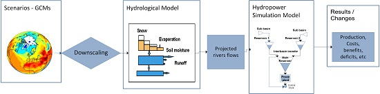
The objective of this study was to evaluate the effects of climate changes on water resources and hydropower production potential in the Kwanza River Basin in Angola. The study evaluates the likely changes in river flows and how these changes would in turn affect the hydropower production potential. The process of assessing effects of climate change involves selecting or defining possible future climate scenarios. Likely future climate scenarios are generated by General Circulation Models (GCMs). The procedure, in general, is that GCM simulations of future climate are used as inputs into hydrological models to evaluate the future changes on river flows to determine impact on water resources. It has been observed that the GCM results are good for large scale assessments, such as global or regional climate change impacts assessments, but not detailed enough to resolve the local scale assessment [16]. This is more so in a region with complex physiographic landscape, where there are pronounced small scale variations in climate variables. Most hydrological models are developed for local scale assessment, resulting in a mismatch between GCM output and the hydrological model requirements. It is therefore usually necessary to downscale to finer resolution suitable for hydrological modelling in the river basins. The process of downscaling fills this gap or mismatch. Downscaling is carried out through different methods; dynamic downscaling or statistical downscaling. Dynamic downscaling is done by using more detailed Regional Climate Models (RCMs). The main advantage of dynamic downscaling is the fact that physical consistency between variables is kept and feedback mechanisms are taken care of in a system. Statistical downscaling, on the other hand, is based on establishing a correlation between large scale GCM results and locally observed climate variables. It presents a computational process that can be carried out more easily by anyone with statistical knowledge and by using a personal computer only. Statistical downscaling has many advantages, including cheap and efficient diagnostics to assess the GCMs skills and reliability [16].

2. Study Area

2.1. Location

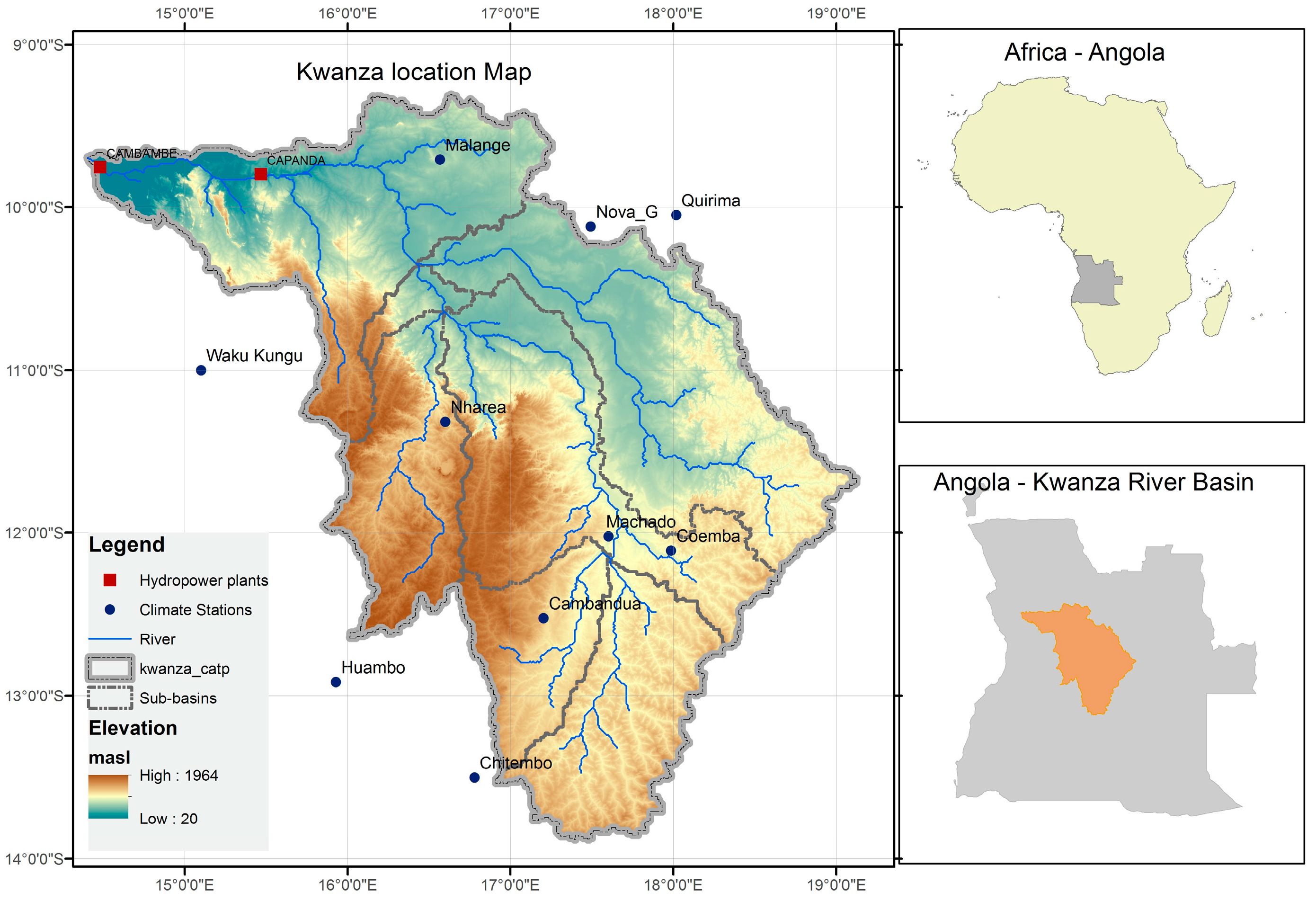
The Kwanza River Basin (also spelled Cuanza or Kuanza), shown in Figure 1, is a river basin in Angola located in the south-western part of Africa within 9°30′ and 13°55′ South and 14°10′ and 19°10′ East. The basin has a total area of about 157,000 km² and borders the catchments of the Cuito and Cubango rivers on the south and southeast. To the east, the Kwanza borders the Zambezi River Basin and its tributaries and to the north and northeast it borders the Congo River Basin. The Kwanza river, approximately 1000 km long, has its source in the Angola highlands (middle of Angola), in the Bie district, at an elevation above 1500 masl. It initially flows northwards and then changes course to the west, near Malanje town. After changing its course, a length of 200 km corresponding to the middle Kwanza, the river rapidly flows down from the Angolan highlands to elevations near sea level, at Cambambe about 60 km south of Luanda.

2.2. Climate and Hydrology

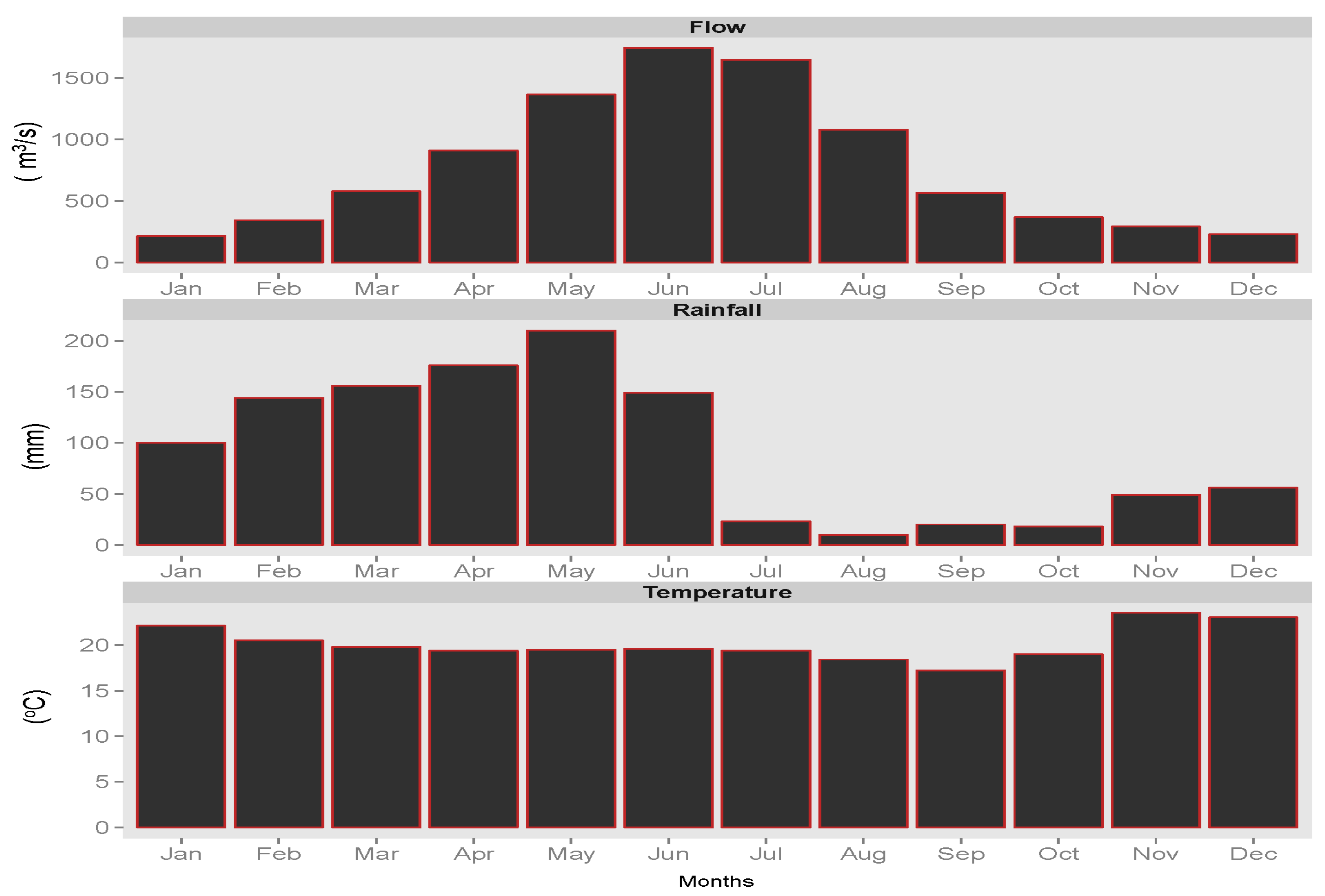
Generally, in Angola, rainfall increases in the northeast direction from the south west bordering the Kalahari Desert. The highest rainfall areas are bordering with Congo in the north-eastern part of the country. Since the Kwanza catchment lies in the centre of the country it therefore enjoys medium to high rainfall. Monthly average rainfall normally reaches the highest values during the months of March to June. The highest annual rainfall is 1490 mm corresponding to the largest flood recorded at Cambambe. The lowest annual rainfall recorded is 828 mm. During the dry season, normally in July–October, there is almost no rainfall. Figure 2 shows mean monthly runoff, rainfall and air temperature over the river basin. The Kwanza basin receives on average 900 mm of annual rainfall with lowest mean of only 400 mm towards to outlet and highest mean of 1400 mm in the highlands. February–June is the main rainy season whereas winter (July–October) is the driest period in the area.

2.3. Hydropower System

The Kwanza River Basin has a large hydropower potential, estimated to be about 6000 MW and it is projected that the basin will be the main source of electricity for Angola when most of the potential is harnessed. Currently, out of the total hydropower potential of 6000 MW, less than 1000 MW is harnessed. The Kwanza hydropower system today has two existing plants. The first hydropower station upstream is the Capanda hydropower plant, comprising a reservoir with a capacity of 4450 million m³, an installed capacity of 520 MW utilizing 640 m³/s and a head of 84 m. The second hydropower station located further downstream is the Cambambe hydropower plant with a smaller reservoir of 20 million m³, an installed capacity of 260 MW using 670 m³/s and a head of 51 m.

The government of Angola has plans to construct two more hydropower plants between these two existing hydropower plants in the near future. These are Nhangue hydropower plant with another reservoir of 3300 million m³; with 1325 MW installed capacity using 625 m³/s and head of 193 m. The second planned hydropower plant is the Cacula Cabasa with an installed capacity of 1025 MW from a head of 191 m using 600 m³/s of flow. Some of the salient features of these hydropower stations are listed in

Table 1. Characteristics of major hydropower projects in Kwanza River Basin, Angola.

Name	Status	Reservoir Million m3	Capacity MW	Design Flow m3/s	Head (m)	Production TWh/Year
Capanda	Operational	4450	520	640	84	2880
Nhangue	Planned	3300	1325	625	193	5732
Cacula Cabasa	Planned		1025	600	191	5440
Cambambe *	Operational	20	260 *	670	51	1440

* The Cambambe power station originally had a rated generation capacity of 260 MW (4 × 65 MW), it only produced 180 MW (4 × 45 MW) due to the low height of the existing dam but dam height was increased by 20 m in 2011 and the plant now operates at 260 MW.

.

3. Methodology

In this study the procedural steps highlighted in Figure 3 were used. The first step in the process was to access the simulation data of relevant global circulation models. Next, these data had to be downscaled to the basin level, in order to be useful as input to the hydrological models. The statistical downscaling technique used was Empirical Statistical Downscaling (ESD). With this method, the expected change in temperature and precipitation in the GCM data can be converted into local changes at climate stations in and around the basin. This computation was implemented in the R statistical software, using the clim.pact package [16]. Empirical-statistical downscaling of GCM output was performed with functions from the R package “clim.pact”. Linear multiple regression was used to establish a statistical relationship between monthly values from station records and the gridded observations. This relationship was further employed to the GCM output for all selected models and emission scenarios. The downscaling was performed at a monthly time step such that the generated output was monthly time series of downscaled mean monthly temperature (°C) and monthly precipitation amount (mm/month).

The HBV hydrological model [17,18] was used to transform climatic variables (temperature and precipitation) to runoff. Finally the nMAG hydropower simulation model [18,19] was used to compute generation in the power plants both for existing and future climate.

The control period was taken 1961–1990. There were no climate stations with good and long term monthly observations of data within the basin, so data from neighbouring (basins) stations was used. Based on results of the comparisons for the control period, were considered to represent climate well. The comparison of GCMs and the observed data, shows that there is good relationship between these although that depends on different GCMs. It is also striking to note that this similarity varies from station to station within Angola. The Taylor diagram was used to make these comparisons [20].

3.1. Hydrological Modelling

For runoff simulation, the HBV hydrological model was used to assess the impact of climate changes on stream flow into Capanda and Cambambe reservoirs. The HBV model [17] is a conceptual rainfall-runoff model which was originally developed for Scandinavian catchments. The model has later been used in very many river basins worldwide, including many tropical basins similar to Kwanza River. It covers the main runoff generating processes using a simple and robust structure with a small number of parameters. The model use Precipitation (P), Air temperature (T) and Potential evaporation as input and computes catchment runoff, typically using daily time-steps. P and T are based on observations while potential evaporation is usually computed from other climatic data. Precipitation input is computed as areal precipitation for the catchment, by combining observations from several stations in or around the catchment, depending on availability. The hydrological model was calibrated using the observed data and later the future climate scenarios for the basin were applied to simulate the projected future flows of the basin.

The HBV hydrological model has been used for hydrological modelling for climate change impacts studies before and has been extensively used in Europe and other parts of the world in a wide range of applications, including climate change studies [21,22,23,24].

Precipitation data was corrected since there is usually a loss of precipitation in the measurement process. In most cases a positive precipitation-elevation gradient will also be used in the model. Air temperature data similar to precipitation are also based on observations at several stations. The areal temperature is computed by taking the arithmetic mean of data from several stations. The temperature decrease with elevation (lapse rate) is usually in the order of −0.6 °C/100 m elevation increase. Increasing or decreasing air temperature will also bring a change in the potential evaporation (PET). Potential-evaporation can be computed by different methods, depending on data availability. Here, the Hargreaves method [25] was used.

3.2. Hydropower Modelling

The results of the hydrological simulations were used as inputs to the hydropower simulation model, the nMAG model developed at NTNU [19]. The nMAG model was developed at NTNU [19] from 1984 to 2004 and was primarily intended for operation simulations to estimate the production and economic benefit of a system under varying hydrological conditions. In addition, it is capable of simulating reservoir operation strategies for an integrated water resources system that includes water supply, irrigation, and flood control projects. The nMAG model system can simulate the production and the economic benefit of a system under the given data on; inflow conditions, production system, consumer system and operation strategy. The model helps to study the economic feasibility of a newly proposed project under varying hydrological and operational conditions. The nMAG hydropower simulation model is simple to use but adequate to representation most of the essential components of a hydropower system. The model contains nodes from four different module types where all or some are contained in a system at a time. These are termed as: Regulation reservoirs, Power plant, Water transfer (Diversions) and Control point. Input data including system reservoir, power plant, bypass, and operation strategy are used to describe the hydropower system for each site. Reservoir evaporation and environmental requirements were specified as well. The time steps of the runoff time series were on monthly time step for some basins and daily time step for the others.

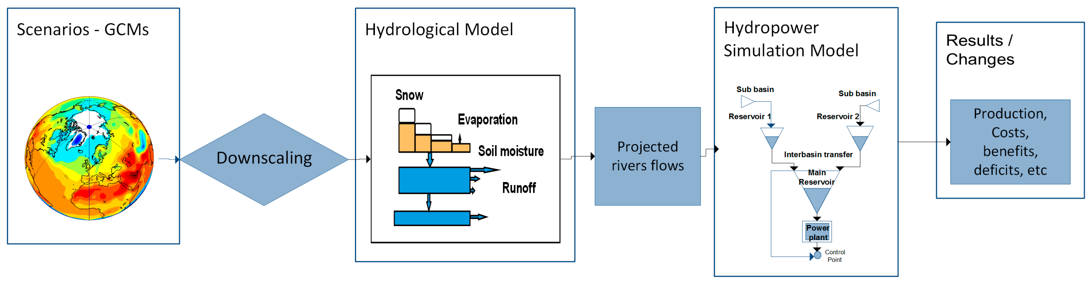
In the model set-up, the existing system consisting (Capanda—520 MW and Cambambe—260 MW) were simulated together with the planned plants with a total production of 15492 TWh/year. The flows resulting from hydrological simulations of the control period (1961 to 1990) were used to simulate the current production levels, and flows from later periods were used for future periods. Figure 4 shows, on the left, the location of existing and planned hydropower plants; and the nMag model setup for Kwanza hydropower system on the right.

4. Data

The source of climate data is one of the IPCC data centre, the Program for Climate Model Diagnosis and Inter-comparison (PCMDI) [26,27]. The data access is free through its data portal [27] through user registration. The data at the centre contains projections of future climate scenarios simulated by the GCMs [28]. Initially five GCMs were selected to be used in the downscaling driven by emission scenarios A1B and B2. A1B emission scenario is regarded to be the medium of the scenarios while B2 is one of the lowest emission scenario. Observed temperature and precipitation data for stations in Angola relevant to the study area were obtained from Global Historical Climatology Network (GHCN) at the National Oceanic and Atmospheric Administration (NOAA) [29]. Most of the climate stations, listed in

Table 2. List of climate stations with monthly rainfall and temperature data.

	Name	Latitude Degrees	Longitude Degrees	Station Code	Elevation masl
1	LUANDA	−8.85	13.23	661601	70
2	WAKU KUNGU (CELA)	−11.42	15.12	662702	130
3	LUBANGO (SA DA BANDEIRA)	−14.93	13.57	663903	1758
4	MENONGUE (SERPA PINTO)	−14.65	17.68	664104	1343
5	MOCAMEDES	−15.2	12.15	664225	45
6	MAVINGA	−15.83	20.35	664476	1088
7	HUAMBO (NOVA)	−12.83	15.83	664318	1708
8	MALANGE	−9.53	16.22	664215	1139

, had short periods of daily data, mostly less than 30 years. For this reason downscaling was carried out on monthly time step. The resulting monthly delta changes from downscaling are then applied to daily data for use in the hydrological modelling. The data from GHCN was used as observed data (predictand) in downscaling process. The company Norsk Hydro AS of Norway provided the available runoff data for the period of 1965–1968 for the basin. However, due to the fact that the data record had a lot of gaps, filling in missing values using data from neighbouring river gauging stations was necessary.

Hydrological parameters required in the modelling, such as the basin area, lake area, and elevation zones were extracted using GIS. Most data describing hydropower plants and systems description was obtained from the company Norsk Hydro AS, in addition some was obtained from the internet. The hydropower system data required included reservoir size (area, volume), installed capacity, efficiency and other parameters.

5. Results

5.1. Hydrological Modelling—Current Period

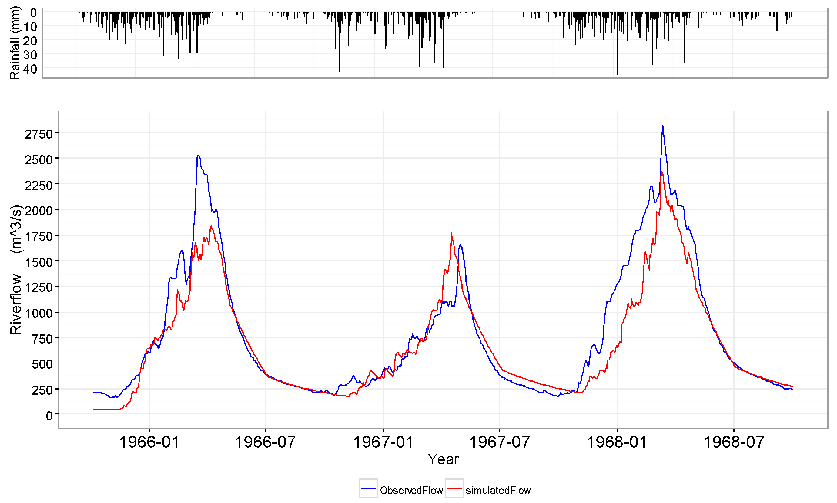
The HBV-model was calibrated for 3 years (1966–1968) using data from observation stations with daily data. The model performance was measured with an objective method based on error function, which defines the goodness of fit, the Nash efficiency criterion, R² and the water balance deviation between the observed and modelled runoff (Q_dev). Optimal model parameters were fine-tuned by manual model calibration after first using an automatic calibration method. The results of model calibration are given in

Table 3. HBV calibration parameters for Kwanza Catchment. Dev. denotes the difference in observed total runoff and the simulated runoff during the calibration period.

Description	Parameter	Value	Units
Rain Correction	PKORR	0.95	-
Elevation Correction	HPKORR	0	-
Field Capacity	FC	120	mm
Beta	BETA	1.33	-
Evaporation threshold	LP	20	mm
Fast Drainage	KUZ2	0.09	mm/day
Slow Drainage	KUZ1	0.02	mm/day
Threshold	UZ1	76	mm
Percolation	PERC	0.98	mm
Drainage Coefficient	KLZ	0.01	mm/day
Model fit	R2	0.85	-
Acc. Difference	Qdev	−88.2	-

that summarizes the final model calibration parameters. The highest R² value is 0.85, a good result for the 3 years with good observations from stations. The calibration of HBV was deemed successful in simulating observed inflow for the runoff observations.

For future climate simulations (2020s, 2050s and 2080s), the change in potential evapotranspiration were computed with respect to temperature for each period. Figure 5 shows the results of the HBV calibration for Kwanza catchment for the period representing the current period.

Figure 5 shows that the model simulations for the calibration period were good although some low runoff years and some peaks are not well simulated. This may be attributed to short periods of data, stations located outside the catchment and poor runoff data available for the basin. In conclusion, despite these deviations, the runoff in the catchment was simulated with acceptable accuracy with the HBV-model.

5.2. Future Climate

The downscaled GCM outputs of precipitation and temperature for the next 90 years were taken from the downscaling results. The future changes are grouped into three distinct periods, namely, the 2020s (2010–2039), the 2050s (2040–2069) and the 2080s (2070–2099). For each station an ensemble of time series are generated with different GCMs and emission scenarios. The comparisons of the changes on future climatic variables were done with respect to the baseline period (1961–1990) and referred to as the current or historical period.

In order to disaggregate the local climate projection into a daily time step, delta change factors were calculated and added to daily time series of observation records. Calculations of delta change factors were based on the difference between the climatology of selected projection intervals (2020s, 2050s and 2080s) and a baseline period (1961–1990) using the Equations (1) and (2). Change factors for temperature were determined by:

$$\Delta T_{i,j,k}={\overline{T}}_{i,j,k}-{\overline{T}}_{ref,k}$$

(1)

where ΔT = Temperature change factor (°C), $\overline{T}$= Monthly mean temperature (°C), i = GCM, j = projection period, and k = month.

Similarly, the equation for estimating precipitation change factors reads:

$$\Delta P_{i,j,k}=\frac{{\overline{P}}_{i,j,k}-{\overline{P}}_{ref,k}}{{\overline{P}}_{ref,k}}\times 100$$

(2)

where ΔP = Precipitation change factor (%), $\overline{P}$= Mean monthly precipitation (mm/month), i = GCM, j = projection period, and k = month. In order to stream line the analysis, it was decided that these ensembles would be aggregated and the median used, even though there were differences.

The analysis here shows that the future climate within and around the Kwanza catchment in Angola will get slightly wetter with higher temperatures than the current period. The northern part of the catchment shows an increase in precipitation while the southern shows a slight decrease in precipitation. The temperature in all places indicates an increase up to 3.2 °C by end of the century. However; the trends vary temporally and spatially, and the rate of increase in the A1B scenario is higher than in B2. The new time series contained the future time series of temperature and precipitation.

5.3. Hydrological Simulations

The HBV model, calibrated with the observed data representing the current period, was also used for hydrological modelling of future runoff series using downscaled temperature and precipitation data. Evaporation potential for the future periods was estimated based on temperature by the Hargreaves method which a modified Thornthwaite method [16]. The calibrated HBV-model was run for the different future climate scenarios and GCMs, to derive future times series of runoff in the 2020s, 2050s and 2080s. Figure 6 shows the general differences between the runoff during the current period and the future periods.

The computed changes in runoff are also shown in

Table 4. Changes in temperature and precipitation and the resulting changes in evaporation and runoff from different GCMs and emission scenarios.

	Precipitation				Temperature
	1961–1990	2030–2045	2050–2080	2081–2099	1961–1990	2030–2045	2050–2080	2081–2099
	mm		% Change		°C		% Change
ECHAM4 B2	1179	−10	6	9	22.3	0.9	1.7	2.1
ECHM5 A1B	1180	−8	16	18	21.4	1.1	1.8	2.9
CCSM3 A1B	1170	−5	6	14	21.7	1.2	1.9	2.6
ECHAM4 A2	1187	−11	18	21	22.3	1.5	2.1	3.4
CCSM3 B2	1184	−3	4	8	21.9	0.7	1.9	2.2
	Potential Evaporation				Total Runoff
	1961–1990	2030–2045	2050–2080	2081–2099	1961–1990	2030–2045	2050–2080	2081–2099
	mm		% Change		mm		% Change
ECHAM4 B2	304	4	8	10	660	4.1	2	8
ECHM5 A1B	306	5	9	11	746	−2.2	3	11
CCSM3 A1B	304	6	10	10	724	−3.0	5	12
ECHAM4 A2	304	7	14	14	687	−2.4	7	16
CCSM3 B2	317	3	8	10	678	−3.4	3	9

for individual scenarios and GCMs, together with predicted changes in precipitation, temperature and evaporation. The runoff changes are not as large as that of rainfall. Referring to Figure 6, the changes in runoff appear to be largest in the later part of the high flow season from April to July, while there is less change in the rest of the year.

5.4. Changes in Flows

The higher flows in occur in the March-April-May (MAM) season (Figure 6) and therefore changes in this season have a greater influence in the overall annual changes. As shown in Figure 7, there is only a slight change in river flow in the MAM season. The overall result is that there is a slight increase in river flow in this basin especially towards the end of the century.

For the future periods, as shown in Figure 7, there is a decrease in runoff in the 2020s and this appears to be for all seasons apart from the DJF season. There is reduction in river flows for MAM and JJA seasons for both the 2020s and 2050s, although in the 2050s, the reduction is small. However when all the season are summed up into annual series, the reduction only appears in the period of 2020s and there are increases in the other two periods in the future.

5.5. Changes in Hydropower Generation

Table 5. Simulation results of the power system and the changes due to climate change for both the B2 and A1B scenarios respectively.

Climate Scenario	Period	Energy Production GWh	Change in Production %
CCSM3 A1B	Present	15,492
	2020s	15,393	−1
	2050s	15,525	1
	2080s	16,094	11
ECHAM5 A1B	Present	15,492
	2020s	15,157	−6
	2050s	16,026	10
	2080s	16,135	12
ECHAM4 B2	Present	15,492
	2020s	15,275	−3
	2050s	15,616	3
	2080s	16,007	10
CCSM3 B2	Present	15,492
	2020s	15,299	−3
	2050s	15,658	4
	2080s	15,809	6

shows the main results from the hydropower simulation model. The table contains average simulated generation for a system with both existing and planned hydropower plants, for different combinations of GCMs, emission scenarios (A1B and B2) and for present and future climate scenarios. The last column contains % change in generation compared to generation under present climate.

Table 6. Average changes in hydropower production Kwanza basin.

Period	Inflow Million m3	Reservoir Evaporation	Inflow Change %	Energy Production GWh/Year	Change %
Current	19,700	220		15,492
2020s	19,306	231	−2	15,222	−3
2050s	21,079	243	7	15,899	4
2080s	22,064	255	12	16,975	10

compares and combines the results from river flow changes and the results of the energy simulation model for different climate scenarios. The average inflow increases towards 2080s after a slight reduction in 2020s, while the reservoir evaporation is increasing steadily throughout the future periods. After the decrease in the 2020s, there is a steady increase in inflows into the hydropower system and a corresponding increase in hydropower production, but the hydropower production does not increase by the same percentage, but slightly less.

6. Summary and Conclusions

Climate change is taking place and will continue to change hydrological cycles. This is the reality. Water resources designers, planners and managers need to take into account the likely changes in water resource availability in the future. The impacts of climate change challenges the investment, planning and operation of the hydropower plants. The analysis done here confirms that there will also be changes in the future climate and hydropower generation potential in the Kwanza River, but the changes are mostly positive.

The temperature over the entire basin is steadily increasing while the precipitation fluctuates a bit, first a decrease in the 2020s and then an increase towards the end of the 21st century. The result of these changes is also increase in evaporation, almost as a direct result of increase in temperature. The projected runoff in the future almost follows the precipitation trend, a decrease in 2020s and gradual increase in the 2050s and 2080s. The result of these changes in the hydrological variables on the hydropower production shows a promising outlook though first a slight decrease. It is seen here that hydropower production could increase up to 10% in the Kwanza River Basin.

Planning of new hydropower and operation of the existing hydropower plants in this basin could take into account some of these likely changes. While the results are indicative of the likely changes, further detailed evaluation with more observed data is highly recommended.

The result of such as a study is dependent on the quality and representativeness of the observed data and the capacity of the employed models for the study. The future climate projection is solely dependent on the ability of the GCM used to simulate the atmospheric variables for the basin studied. It is recommended that future work should include more stations in the basin to get better spatial coverage and the output of multiple GCMs for future climate projection to see the level of uncertainty in the outcome. During the downscaling, precipitation downscaling was more challenging than temperature; hence, it is recommended to use additional downscaling methods to get a better result. The use of regional climate models, when available over Africa, is highly recommended. Finally, for the hydropower simulation, more recent data for the plants and for the other demands (irrigation and water supply) should be used in the future analysis.

Lack of good observed data highlighted some of the challenges the basin or country (region) faces and this limits the applicability of modelling tools for impact assessments. In this study the downscaling and hydrological modelling were limited by the short length of observed data. There is need for improved collection of both climate and hydrological data in the basin. While this study attempted to take into account the main water users (water supply, irrigation), the future estimates proved difficult to estimate. Future developments and the estimation of water demand need to be taken into account when similar analyses are carried out.

References

- Arnell, N.W.; Livermore, M.J.L.; Kovats, S.; Levy, P.E.; Nicholls, R.; Parry, M.L.; Gaffin, S.R. Climate and socio-economic scenarios for global-scale climate change impacts assessments: Characterising the SRES storylines. Glob. Environ. Chang. 2004, 14, 3–20. [Google Scholar] [CrossRef]
- Gleick, P. The World’s Water 2008–2009; Technical Report; Pacific Institute for Studies in Development, Environment, and Security: Washington, DC, USA, 2008. [Google Scholar]
- Christensen, J.H.; Hewitson, B.; Busuioc, A.; Chen, A.; Gao, X.; Held, I.; Jones, R.; Kolli, R.K.; Kwon, W.T.; Laprise, R.M.; et al. Regional Climate Projections; Technical Report; Intergovernmental Panel on Climate Change (IPCC): New York, NY, USA, 2007. [Google Scholar]
- Menne, M.J.; Williams, C.N., Jr. Homogenization of temperature series via pairwise comparisons. J. Clim. 2009, 22, 1700–1717. [Google Scholar] [CrossRef]
- Sillmann, J.; Roeckner, E. Indices for extreme events in projections of anthropogenic climate change. Clim. Chang. 2008, 86, 83–104. [Google Scholar] [CrossRef]
- De Wit, M.; Stankiewicz, J. Changes in surface water supply across Africa with predicted climate change. Science 2006, 311, 1917–1921. [Google Scholar] [CrossRef] [PubMed]
- Lobell, D.B.; Bonfils, C.; Duffy, P.B. Climate change uncertainty for daily minimum and maximum temperatures: A model inter-comparison. Geophys. Res. Lett. 2007, 34. [Google Scholar] [CrossRef]
- Timmermann, A.; Lorenz, S.; An, S.I.; Clement, A.; Xie, S.P. The effect of orbital forcing on the mean climate and variability of the tropical pacific. J. Clim. 2007, 20, 4147–4159. [Google Scholar] [CrossRef]
- Hamududu, B.; Killingtveit, A. Assessing climate change impacts on global hydropower. Energies 2012, 5, 305–322. [Google Scholar] [CrossRef] [Green Version]
- Yamba, F.; Walimwipi, H.; Jain, S.; Zhou, P.; Cuamba, B.; Mzezewa, C. Climate change/variability implications on hydroelectricity generation in the zambezi river basin. Mitig. Adapt. Strateg. Glob. Chang. 2011, 16, 617–628. [Google Scholar] [CrossRef]
- Andersson, L.; Julie, W.; Martin, T.C.; Denis, H.A.; Earle, A.K.; Russel, D.L.; Hubert, S.H.G. Impact of climate change and development scenarios on flow patterns in the okavango river. J. Hydrol. 2006, 331, 43–57. [Google Scholar] [CrossRef]
- Folwell, S.; Farqhuarson, F. The Impacts of Climate Change on Water Resources in the Okavango Basin; International Association of Hydrological Sciences (IAHS) Press: Wallingford, UK, 2006; pp. 382–388. [Google Scholar]
- Hamududu, H.B. Impacts of Climate Change on Water Resources and Hydropower Systems in Central and Southern Africa. Ph.D. Thesis, Norwegian University of Science and Technology, Trondheim, Norway, 2012. [Google Scholar]
- Hughes, D.A.; Andersson, L.; Wilk, J.; Savenije, H.H.G. Regional calibration of the pitman model for the okavango river. J. Hydrol. 2006, 331, 30–42. [Google Scholar] [CrossRef]
- Andersson, L.; Samuelsson, P.; Kjellström, E. Assessment of Climate Change Impact on Water Resources in the Pungwe River Basin. Tellus A 2011, 63, 138–157. [Google Scholar] [CrossRef]
- Benestad, R.E.; Haugen, J.E. On complex extremes: Flood hazards and combined high spring-time precipitation and temperature in Norway. Clim. Chang. 2007, 85, 381–406. [Google Scholar] [CrossRef]
- Bergstrom, S. Development and Application of a Conceptual Runoff Model for Scandinavian Catchments; Swedish Meteorological and Hydrological Institute (SMHI): Norrköping, Sweden, 1972. [Google Scholar]
- Killingtveit, A.; Saethun, N.R. Hydrology; Norwegian Institute of Technology, Division of Hydraulic Engineering: Trondheim, Norway, 1995. [Google Scholar]
- Killingtveit, A. nMAG User Manual; Norwegian Institute of Technology, Division of Hydraulic Engineering: Trondheim, Norway, 2004. [Google Scholar]
- Taylor, K.E.; Stouffer, R.J.; Meehl, G.A. An Overview of CMIP5 and the experiment design. Bull. Am. Meteorol. Soc. 2012, 93, 485–498. [Google Scholar] [CrossRef]
- Bergström, S.; Johan, A.; Noora, V.; Bertel, V.; Bergur, E.; Sveinbjörn, J.; Liga, K.; Jurate, K.; Diana, M.B.; Stein, B.; et al. Modelling Climate Change Impacts on the Hydropower System; Climate Change and Energy Systems Impacts, Risks and Adaptation in the Nordic and Baltic Countries; Technical Report; Nordic Council of Ministers: Copenhagen, Danmark, 2012. [Google Scholar]
- Bergstrom, S.; Andreeasson, J.; Veijalainen, N.; Vehvilainen, B.; Einarsson, B.; Jonsson, S.; Kurpniece, L.; Kriauciuniene, J.; Meilutyte-Barauskeine, D.; Beldring, S.; et al. Climate Change and Energy System; Impacts, Risks and Adaptation in the Nordic and Baltic Countries; Technical Report; Nordic Council of Ministers: Copehagen, Danmark, 2011. [Google Scholar]
- Bergstrom, S.; Carlsson, B.; Gardelin, M.; Lindstrom, G.; Pettersson, A.; Rummukainen, M. Climate change impacts on runoff in sweden; assessments by global climate models, dynamical downscaling and hydrological modelling. Clim. Res. 2001, 16, 101–112. [Google Scholar] [CrossRef]
- Saelthun, N.R. Nordic HBV Model. Description and Documentation of the Model Version Developed for the Project Climate Change and Energy Production; Technical Report; Nordic: Oslo, Norway, 1996. [Google Scholar]
- Hargreaves, G.H.; Allen, R.G. History and evaluation of Hargreaves evapotranspiration equation. J. Irrig. Drain. Eng. 2003, 129, 53–63. [Google Scholar] [CrossRef]
- Taylor, K.E. Summarizing multiple aspects of model performance in a single diagram. J. GeoPhys. Res. 2001, 106, 7183–7192. [Google Scholar] [CrossRef]
- Program for Climate Model Diagnosis and Intercomparison (PCMDI). Available online: http://cmip-pcmdi.llnl.gov/cmip5/data_portal.html (accessed on 4 May 2011).
- Intergovernmental Panel on Climate Change. Climate Change 2007: The Physical Science Basis. Contribution of Working Group I to the Fourth Assessment Report of the Intergovernmental Panel on Climate Change; Technical Report; Intergovernmental Panel on Climate Change (IPCC): Geneva, Switzerland, 2007. [Google Scholar]
- Global Historical Climate Network (GHCN). Available online: http://www.ncdc.noaa.gov/ghcnm/v3.php (accessed on 5 March 2009).
© 2016 by the authors; licensee MDPI, Basel, Switzerland. This article is an open access article distributed under the terms and conditions of the Creative Commons Attribution (CC-BY) license (http://creativecommons.org/licenses/by/4.0/).