Code-to-Code Validation and Application of a Dynamic Simulation Tool for the Building Energy Performance Analysis

Abstract

In this paper details about the results of a code-to-code validation procedure of an in-house developed building simulation model, called DETECt, are reported. The tool was developed for research purposes in order to carry out dynamic building energy performance and parametric analyses by taking into account new building envelope integrated technologies, novel construction materials and innovative energy saving strategies. The reliability and accuracy of DETECt was appropriately tested by means of the standard BESTEST validation procedure. In the paper, details of this validation process are accurately described. A good agreement between the obtained results and all the reference data of the BESTEST qualification cases is achieved. In particular, the obtained results vs. standard BESTEST output are always within the provided ranges of confidence. In addition, several test cases output obtained by DETECt (e.g., dynamic profiles of indoor air and building surfaces temperature and heat fluxes and spatial trends of temperature across walls) are provided.

1. Introduction

Since the early 1970s, building energy performance simulation (BEPS) tools have played a crucial role in the assessment of the environmental and energy-related impacts of buildings, which represent the largest energy consuming sector in the developed world [1]. Specifically, due to the growing concern about the energy efficiency of buildings, a significant number of simulation tools has been developed and adopted to support efficient design or redesign, construction or refurbishment, and operation of energy efficient buildings. Such tools also allow dealing with all the most important phenomena occurring in the building itself [2,3,4] and among it and the applied energy efficiency techniques or renewable energy sources [5]. As a result, dynamic simulation is a well-recognized method for the assessment of the building energy performance. The use of dynamic simulations is particularly crucial during the very early stages of the building design, as well as during the refurbishment process of existing buildings (where full scale testing campaigns are costly and/or not practicable). The adoption of BEPS tools is more and more crucial and highly recommended for the design of the next generation of buildings (NZEBs), for the promotion of the integration of renewable energy technologies and for the building energy diagnosis [6,7].

Although BEPS tools have been in use throughout the building energy community for decades, their adoption has been boosted by the recent advances in computational methods and computer calculation power, that have provided key opportunities also for the enhancement of such tools and for the development of new ones [8]. In fact, despite of the availability of commercial BEPS tools and codes, more and more up to date tools (mainly conceived for research applications) have been developed (e.g., [9,10,11]) with the intention of providing greater design flexibility while accomplishing the challenging multiple aim of [12]: (i) investigating new unreleased energy efficiency measures and strategies, (ii) meeting the highest expectations for the comfort of occupants, (iii) increasing models’ robustness and fidelity also toward the implementation of innovative control strategies [13]. Moreover, novel BEPS tools, also coupled to commercial ones, are constantly being developed to help the definition and development of the next generation of buildings [5], to be designed through suitable computer-based analyses [14,15].

Despite the number of new developed tools and codes and the wider and wider adoption of dynamic BEPS tools, building energy simulation is still nowadays a complicated process that requires modeling and analytical skills for both the development and use phases. As an example, the use of BEPS tools and the analysis of the related results can be considered as a challenge for building designers and practitioners who are sometimes bewildered by the selection of a suitable BEPS tool and by the uncertainty about the fidelity of the calculation results [12]. Therefore, novel in-house developed BEPS tools must be validated in order to ensure reliable and accurate energy analyses and to prevent a negative impact on the acceptance of the obtained results. Nevertheless, as well known, despite of the advancements in validation methodologies for building energy simulation tools, the validation process is still time consuming and rather difficult to accomplish [16]. It is also worth noting that while the validation of a single mathematical model for the energy performance analysis of a new building technology, component or material, can be often easily assessed, the experimental validation of a whole BEPS code is not always feasible and currently practicable. This is particularly true for the new generation of dynamic building simulation codes that must be capable of simulating a variety of innovations which would require extensive extremely costly and time consuming testing procedures [5,17]. Note that, accurate energy analyses often could not be ensured by simply adding to existing BEPS codes new subroutines, suitably developed for simulating innovative technologies and investigating their effectiveness. In any case, at the end of the entire modeling process a validation of the whole BEPS code is always necessary and recommended [12].

In this regard, in order to validate novel BEPS tools, several general criteria and standard procedures have been developed and are available in [18]. They consist of comprehensive and integrated suites of building energy analysis tool tests, involving analytical, comparative, and empirical methods. Their adoption has been recently emphasized by the energy performance building directive (EPBD) issued by the European Union that underlines the need of new certified tools to be developed for decision-makers and practitioners in order to provide integrated building design applications and to obtain the compliance with higher energy efficiency standards.

One of the most important international standard tools conceived in order to increase the confidence of BEPS code outcomes is the Building Energy Simulation TEST (BESTEST) procedure [19]. This validation method was purposely developed for testing, diagnosing and validating the capabilities of new BEPS tools. The BESTEST procedure consists of suitable analytical techniques and tests to be carried out for the comparison of the results obtained thorough a novel BEPS program or design tool with those obtained by the current state-of-the-art codes. Recently, a number of the BESTEST cases have been incorporated into ANSI/ASHRAE Standard 140-2011 [20]. Note that, the International Energy Agency (IEA) assumed the BESTEST as the official standard procedure for the new BEPS codes validation. The BESTEST procedure was also adopted by the European Committee for Standardization (CEN) as the test for checking the reference cooling load and energy calculation methods, based on the requirements of several standards addressing different aspects of the EPBD [21]. Through the BESTEST and similar procedures, many new BEPS codes were validated [22,23,24].

Although different mathematical models and assumptions adopted in the available BEPS codes (e.g., for assessing the occurring building physic phenomena), by following the above mentioned validation approach all the occurring bugs can be detected and fixed. At the end of the validation procedure, reliable predictions of the system behavior can be obtained in terms of: (i) energy use for heating, cooling, lighting, etc.; (ii) operating temperatures of the building elements and indoor air; (iii) occupants’ indoor comfort.

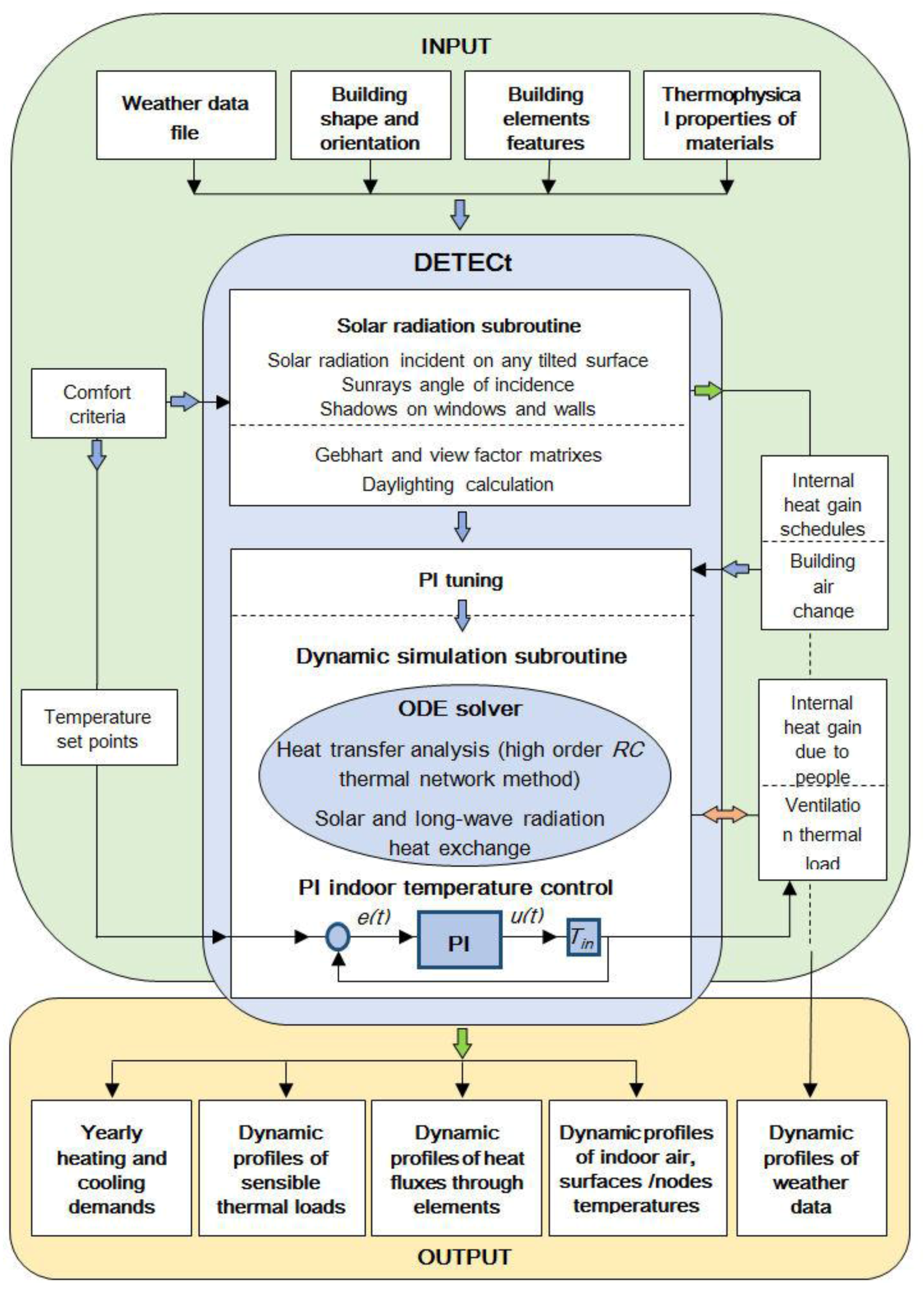
This paper is focused on this framework. In particular, it describes the most important steps and outcomes obtained by following the BESTEST validation procedure, purposely adopted for the diagnosis and validation of a dynamic BEPS tool, named DETECt and developed for research aims by Buonomano and Palombo [25]. This code is able to dynamically predict the thermal behavior of mono and multi-zone (and multistory) buildings and to assess the benefits of different and advanced building envelope techniques in case of different weather locations, envelope materials (also including integrated phase change materials and solar based technologies), building shapes, orientations and geometries. DETECt was implemented in a computer code written in MatLab [26]. The tool and the code are not yet available for use and inspection by any users. Nevertheless, since DETECt was expressly developed for research aims, it has been used and inspected by several researchers (with different backgrounds) for the implementation of novel features. From this point of view, by means of DETECt, novel building envelope technologies or plant/systems and control strategies were implemented and studied by the authors and by several researchers [27,28,29]. The authors are also working on a future freely available release of the tool with a suitable user friendly interface.

The BESTEST procedure adopted for the validation of DETECt (e.g., in case of the basic mono-zone building) was selected on the basis of several criteria, such as completeness, accuracy, reproducibility and cost effectiveness of the test suite. In fact, this procedure consists of widely available high quality empirical validation data sets and it includes detailed and unambiguous documentations of the input data for a selected number of representative design conditions.

The outcomes of this paper refer to several main topics, such as: (i) comparison of DETECt results vs. the mandatory BESTEST qualification cases (in terms of heating and cooling annual energy demand and integrated peak-load, annual transmitted and incident solar radiation, annual hourly zone temperature); (ii) results and discussion regarding the assessment of some hourly variables and their comparison vs. the reference trends; (iii) description of the iterative refinement process carried out for minimizing the sources of the divergences, detected during the validation tests and occurred among the results obtained by the presented code and the reference ones.

DETECt surpassed the BESTEST reliability test. In particular, low or very low deviations of the results obtained by the novel presented code vs. those provided by the validation procedure are observed. Note that an additional code to code validation test, purposely conceived for several commercial buildings located in different weather locations, was also carried out [25]. The development of the presented model and the correspondent code validation were obtained after several years of research work and the activity of modeling innovative technologies for building envelopes and HVAC systems, to be implemented in DETECt, is still today extant.

In the paper, some original examples concerning the capability of the presented code to assess the building energy performance are also reported. Some graphics about the temperature and heat fluxes dynamic trends and spatial temperature gradients into walls are also reported.

2. Model Description

2.1. Framework and General Model Description

The fidelity and accuracy of the simulation results obtained through a BEPS tool depend on the mathematical models and assumptions adopted for the description of the occurring building physical phenomena [30]. Usually, in order to develop straightforward tools, only a few system phenomena are modeled and only the most significant physical aspects occurring in the dynamic building thermal behavior are taken into account. For example, in some building simulation models the conduction heat transfer is solved by lumping all the building thermal masses in a single node of a considered thermal network, avoiding the adoption and the resolution of many partial differential equations [31]. Nevertheless, these simulation approaches because of their reliability do not allow one to obtain details about the building surfaces temperatures, necessary for comfort analyses and for simulating the frequent rapid variation of the thermal conditions occurring in buildings [32]. Moreover, in the last years, the research in the building energy saving field as led to the investigation of new building integrated technologies and innovative heating, ventilating and air conditioning (HVAC) systems often supported by renewable energies or innovative control strategies [33]. Thus, in order to analyze the energy performance of innovative building plant systems and to predict the whole building thermodynamic behavior, more and more suitable detailed mathematical algorithms/models for computer-based simulation and optimization analyses are being developed and used [11,22,24,34]. In general, in detailed building models, the energy response of each thermal zone is suitably analyzed by taking into account almost all the physical phenomena. A summary of the assumptions, features and limitations of such models are reported in [13,35,36].

The building simulation model here described has been developed by taking into account the above described framework [25,28]. The model is based on a nodal description of the building elements with a one dimensional modelling of the thermal phenomena occurring in the building (i.e., transverse heat transfer often plays a minor role in the building conduction phenomena [37]). In addition, in order to analyze the effect of the spatial distribution of the heat capacity on the heat flux through the building envelope elements, the thermal network approach, based on a high number of thermal capacitances is taken into account (i.e., distributed parameters model [38]). Therefore, in DETECt, numerical simulations are based on a transient lumped parameters heat transfer model, which enables an accurate simulation of dynamic effects driven by the thermal mass. DETECt is able to simulate the temperature and flux fields of a mono-zone and multi-zone (as well multistory) building according to the climate, once building orientation, constructive and operation features and climate are selected. Through the code, the dynamic calculation of the indoor air and building surfaces temperatures, also useful for comfort analyses, can be assessed.

The code was developed with the help of the MatLab platform [39], selected due to its high performance on numerical computation, visualization, and programming (which allow one to easily analyze data, develop algorithms, and create models and applications) as well as to its high flexibility with respect to the controller development (enabling the integration of new and advanced controllers). The also platform includes built in solvers for differential equations systems and math functions which aid exploring multiple approaches (including advanced control analyses) and reach faster solutions than traditional programming languages.

The detailed description of the theoretical engine implemented in the presented tool, as well as the simulator logic, is described in the following. Specifically, the simulation code is subdivided in several sub-models, as summarized in the block diagram of Figure 1. Here, the core of the dynamic calculation procedure is also shown. Specifically, the main sub-models of the simulation code, grouped in a single calculation tool, regard: (i) the calculation of the Sun’s path and the solar irradiance incident on building envelope surfaces; (ii) the resolution of the heat transfer process. The input data of the simulation code are: hourly weather data (temperature, humidity, global and direct normal radiation), occupancy loads and schedules, ventilation flow rate, temperature set points, building size and orientation, thermal features of the building elements (conductivity, density, specific heat, absorption and emission coefficients, etc.). Such inputs can be easily implemented by means of a script in which data about building dimensions, number of thermal zones, thermal features (e.g., including density, heat capacity and conductivity of layers of the envelope), etc. are input in the form of vectors or scalars. Regarding the building envelope features, built-in sets of materials and properties are also available for easy selection. Once the main external dimensions of the building and the number of stories/zones and windows is defined, together with the definition or selection of opaque and transparent properties, the building (as well as the set of buildings to be simulated) is automatically modeled. In addition, a collection of weather data is included in the code, though any weather data file can be easily included by the user in the code as .txt file, obtained by available databases (e.g., Meteonorm, Typical Meteorological Year (TMY), etc.). Conversely, the simulation outputs are instead obtained in the format of images and text files (e.g., .txt and .xls) and can be chosen according to the specific needs of the user. As an example, in addition to heating and cooling loads and yearly requirements, some graphical tool results can be obtained, such as the dynamic trends of temperatures (for indoor air and building elements surfaces and layers) and energy demands, as well as spatial temperature gradients into walls. The presented tool can be also coupled to additional codes for plant simulation (including renewable technologies) for a whole building-plant simulation. Two examples implementing a simpler model for the building envelope energy analysis are reported in [29,40].

In the next sections, a brief description of the most important phenomena included in the code is provided with the twofold aim of better discussing the engine logic and to show the adopted mathematical models and assumptions that primarily influence the fidelity and accuracy of the simulation results.

2.2. Heat Flow Calculation Procedure

DETECt is based on a nodal description of a building with a 1D transient conduction model adopted for the description of the transient heat transfer through the building elements of each thermal zone. By adopting the finite difference method and assuming a one-dimensional thermal domain, the building is subdivided into Z different thermal zones. In each thermal zone the indoor air is considered as uniform and modeled as a single indoor air temperature node, whereas the zone envelope is split into M multi-layer elements (wall, floor, roof, horizontal and vertical internal partition and window), modeled through a suitable thermal resistance capacitance (RC) network. Here, each building element construction material is considered as uniform and therefore its thermal mass and conductivity are uniformly discretized into a number of layers. Thus, each building element is discretized into a suitable number, N, of thin sub-layers of different thicknesses. In each sub-layer, represented with a single node of the considered thermal network, a uniform temperature is assumed. The sub-layer includes two conductive resistances and a single lumped capacitance. For each m-th building element two additional surface non-capacitive thermal nodes are taken into account and considered as boundary nodes (linked to the outdoor and indoor air temperatures). In Figure 2 the scheme considered for the N + 2 nodes thermal network of the generic m-th building element is depicted. Since interface contact resistances are neglected, a perfect thermal contact of each adjacent inner homogeneous material layer to the connected ones is always supposed (i.e., identical interfacial temperatures are hypothesized). Here, homogeneous, isotropic and time-invariant thermo-physical properties (density, specific heat and conductivity) are assumed. The heat transfer taking place out of each m-th building element occurs by convective and radiative equivalent thermal resistances, Figure 2. In this figure, for the sake of simplicity, the external and internal solar radiation fluxes are reported as thermal loads, ${\dot{Q}}_{sol}$ and ${\dot{Q}}_{sol,tran}$. Therefore, in order to assess the building thermal response, the system including all building thermal zones is modeled through a thermal network of Zx((N + 2)xM + 1) nodes. Note that the dynamics of the whole set of node temperatures are described by the differential and algebraic equations taking into account the internal and external solicitations. Obviously, the higher the number of sub-layers, the lower the sub-layer thickness and capacity and through a high number of nodes the discretized model tends to become identical to the physical one (the accuracy of the simulation results improves and high temperature gradients can be obtained) [38]. On the other hand, beyond a certain N number the enhancement of the simulation results fidelity becomes negligible.

The simulation time domain is subdivided into a large number of discretized time steps. The solution of the set of simultaneous equations (described in the following) is carried out iteratively throughout the whole number of such integration sample times. Specifically, the number of time steps has to be selected with regard to the requested simulation fidelity and calculation efficiency. Note that the computation accuracy improves by increasing the number of time steps, whereas too long computational times could be necessary.

For all such reasons, in the presented model the number of thermal network nodes and simulation time steps depend on the trade-off between the desired calculation accuracy and simulation time, concurrently). Typically, in such kind of calculation procedures, a maximum sub-layer thickness of 1 cm and sample time about 300 s are taken into consideration [41].

Note that, thanks to the efficiency of numerical integration methods as well as to the nowadays powerful computational systems and tools, long standing finite difference methods can be employed for the solution of such set of ordinary differential equations (ODE). In DETECt such equations are solved by a suitable tool, such as a built-in ODE solver included in MatLab, which employs variable step size Runge-Kutta and trapezoidal rule integration methods [39]. In each interval of integration the error of time discretization is within a given range of tolerance, whereas the convergence criteria need to be satisfied within the selected maximum time step.

In DETECt, for each z-th thermal zone and in each τ-th time step, the differential equation describing the energy rate of change of each capacitive n-th node (1 ≤ n ≤ N) of the m-th building element (1 ≤ m ≤ M) is:

$$C_{m,n}\frac{d{T}_{m,n}}{dt}={\displaystyle \sum _{j=n-1}^{n+1}\frac{T_{m,j}-T_{m,n}}{R_{m,j\cdot n}^{cond}}}+\mathsf{\gamma }\cdot {\dot{Q}}_{m,n}^{rad}$$

(1)

where C and T are the thermal capacitance and the temperature of the generic node, $R^{cond}$ is the sum of the halves sub-layers thermal resistances that couples the n-th node to their neighbor ones. Such total resistance is coincident with that one of half sub-layer if the capacitive nodes are coupled to the surface non-capacitive ones. For such outer (n = 0) and inner (n = N + 1) surface non-capacitive nodes, Figure 2, the algebraic equation describing the related heat transfer is obtained by Equation (1) setting the thermal capacitance $C_{m,n}$ to zero. ${\dot{Q}}^{rad}$ is the radiative forcing function, only acting on acting non-capacitive nodes (γ ≠ 0 if n = 0 or n = N + 1, being γ = 0 elsewhere), below described. Note that, for the calculation of the convective resistances, the outdoor and indoor surface unitary convection heat transfer coefficients can be either set as constant depending on the surface type (rough, smooth, very smooth/glass, etc.) or optionally calculated, for rough surface, by empirical relationships. More details are reported in [25,28].

The energy rate of change linked to the indoor air mass depends on the difference between the energy supplied to and removed from it. Thus, differential equation on the thermal network node of the indoor air (which must be solved simultaneously with the system of Equation (1)) is calculated as:

$$C_{in}\frac{d{T}_{in}}{dt}={\displaystyle \sum _{m=1}^M\frac{T_{m,N}-T_{in}}{R_{m,\text{int}}^{conv}}}+{\dot{Q}}_{gain}+{\dot{Q}}_{vent}\pm {\dot{Q}}_{hc}$$

(2)

where $C_{in}$ is the thermal capacitance of the zone indoor air, whose temperature, $C_{in}$, is assumed as homogeneous in the space. The heat exchange between the M internal surfaces nodes and the indoor air one is proportional to the internal convective resistances, $R^{conv}$, calculated as a function of the surfaces condition (e.g., ascendant or descendant flow, wall inclination).

In DETECt, with exception of the radiative thermal load, all the sensible heat gains are networked to the indoor air node only (as purely convective). Specifically, the following assumptions are taken into account:

(1)

The thermal zone internal load due to occupants (i.e., the metabolic rate depends on the indoor air temperature), lights and equipment, ${\dot{Q}}_{gain}$, is modeled as a lumped convective sensible heat source. The internal gains due the occupants can be also calculated as a function of the selected occupants’ behavior schedules. Such schedules can also be connected to the human control of windows solar shadings, infiltration and indoor air temperature set points. Clearly, these parameters have a direct and indirect influence on the building energy demands.

(2)

The ventilation thermal load ${\dot{Q}}_{vent}$ is proportional to the air mass flow rate, ${\dot{m}}_{vent}$, including both the infiltration and ventilation terms and to the difference between the indoor air temperature and the outdoor one T_out.

(3)

The sensible heat to be supplied to or to be removed from the building space by an ideal heating and cooling system, ${\dot{Q}}_{hc}$, necessary to maintain the indoor air at the desired set point temperatures, is calculated according through a proportional integral (PI) controller (widely adopted in buildings for heating and cooling systems control [42]). The indoor air temperature can be controlled to a fixed set point or free to float in an allowed interval avoiding the activation of the ideal heating and cooling system. The control target is achieved by a linear PI driven by a calculated error signal, e(t), i.e., deviation between the indoor air temperature and the set point one, T_sp. In DETECt, the proportional, K_p, and integral, K_i, parameters gains of such PI control are linearly varied as a function of the steady-state heating and cooling demands (ranging from zero—system stand-by—to the space design/peak heating and cooling loads). Such design loads are previously calculated at the beginning of each simulation by following the ASHRAE methods [43]. With the aim to track the set point temperature, the sensible load ${\dot{Q}}_{hc}$ is governed by the output control signal u(t), which range from 0 (i.e., system stand-by) to 100% (i.e., proportional to the design heating and cooling load of the space) [44]. Specifically, the proportional gains are calculated as the ratio of the maximum controlled system output (peaks of ${\dot{Q}}_{hc}$) to the throttling range, i.e., $\left|\min (T_{in})-T_{sp}\right|$ for the heating mode and $\left|\max (T_{in})-T_{sp}\right|$ for the cooling one [44]. The integral gain, added to the controller with the aim to eliminate the offset caused by the proportional gain, is tuned by assuming a time scale ($K_p/K_i$) equal to the simulation time step [45]. The linear resultant of the proportional and integral error at time t is the control signal u(t) of the PI controller. u(t) and e(t) are calculated as:

$$u(t)=K_p\cdot e(t)+K_i\cdot {\displaystyle \underset{0}{\overset{t}{\int }}e(t)dt} \text{and} e(t)=(T_{sp}-T_{in})$$

(3)

For a very high number of simulations, the PI controller has been tested for many system operating conditions, resulting stable and robust also for a wide range of conditions and under typical system dynamic changes.

(4)

Initial and boundary conditions on the thermal network are set as a function of the building element position and the occurring forcing functions, temperatures and solar radiation (only acting on the surfaces of each m-th building element). While the outdoor/indoor temperatures (depending on the adjacency of the z-th zone) are taken into account through the above discussed convective resistances, the radiative forcing functions are comprised in the thermal source ${\dot{Q}}^{rad}$. Specifically, it is assumed as acting on the outer (n = 0) and inner (n = N + 1) surfaces of each m-th building element, which can be considered as adjacent to: (i) an indoor thermal zone; (ii) the outdoor space conditions. When the m-th building element separates two eventually heated or cooled thermal zones on its outer surface the only considered boundary condition is the indoor air temperature of the related adjacent space. Conversely, in case of an external outer surface the considered boundary conditions are the outdoor air temperature, the radiation exchange with the sky vault and the solar radiation, all provided in the weather data file. On external opaque and glazed surfaces, the forcing function (${\dot{Q}}_{m,0 }^{rad}$) includes both the solar and long wave radiations, while on inner opaque and glazed surfaces (as well as on internal facing surfaces of the gap of multi-layered glazing system), the forcing function (${\dot{Q}}_{m,N+1 }^{rad}$) takes into account the solar radiation incident on the surface, due to the solar radiation load entering through windows and the net long wave radiation load received by the other i-th (1 ≤ m ≤ M) internal surfaces of the considered thermal zone. Such terms, for each m-th element of A heat exchange surface area, are calculated as:

$$\begin{array}{l} {\dot{Q}}_{m,0 }^{rad}=\left[{\mathsf{\epsilon }}_m^{ext}\cdot \mathsf{\sigma }\cdot f\cdot (T_{sky}^4-T_{m,1}^4)+{\mathsf{\alpha }}_m^{ext}\cdot I_m^{ext}\right]\cdot A_m \\ {\dot{Q}}_{m,N+1 }^{rad}=\left[{\mathsf{\epsilon }}_m^{int}\cdot \mathsf{\sigma }\cdot {\displaystyle \sum _{i=1}^M{G}_{bm}\cdot (T_{i,N}^4-T_{m,N}^4)} +{ \mathsf{\alpha }}_m^{int}\cdot I_m^{\mathrm{int}} \right]\cdot A_m\end{array}$$

(4)

where f is the external surface view factor, $T_{sky}$ is the sky temperature, ε and α are the selected emissivity and absorption factors; I is the total solar radiation flux.

The solar radiation entering through glasses is absorbed, reflected and distributed within the internal space by selected absorption, reflection and view factors, respectively. $I_m^{\text{int}}$ is the total solar radiation flux striking an internal m-th surface and it includes the solar irradiance reflected by other interior surfaces. Such flux is the m-th component of the total solar radiation flux vector, $I^{int}$, which is calculated as:

$$\left(\begin{array}{c}{I}_1^{int}\\ I_2^{int}\\ \cdots \\ I_M^{int}\end{array}\right)={\left(\begin{array}{cccc}\left(1-F_{11}{\mathsf{\rho }}_1^S\right)& -F_{12}{\mathsf{\rho }}_2^S& {-}_{\cdots }& -F_{1M}{\mathsf{\rho }}_M^S\\ -F_{21}{\mathsf{\rho }}_1^S& \left(1-F_{22}{\mathsf{\rho }}_2^S\right)& {-}_{\cdots }& -F_{2M}{\mathsf{\rho }}_M^S\\ \cdots & \cdots & \cdots & \cdots \\ -F_{M1}{\mathsf{\rho }}_1^S& -F_{M2}{\mathsf{\rho }}_2^S& {-}_{\cdots }& \left(1-F_{MM}{\mathsf{\rho }}_M^S\right)\end{array}\right)}^{-1}\cdot \left(\begin{array}{c}{I}_1^0\\ I_2^0\\ \cdots \\ I_M^0\end{array}\right)$$

(5)

where the generic F and ${\mathsf{\rho }}^S$ are the internal surfaces view factors and the solar reflectivity coefficients. F is automatically calculated for parallelepiped structures [46]. $I^0$ is the vector of the solar radiation directly received by the interior surfaces and is subjected to the solar radiation effectively transmitted through windows (depending on the equivalent solar transmission coefficient of the glazed surfaces). The coefficients of the $(\overline{I}-F\cdot P_S)$ matrix reported in Equation (5) are calculated only at the beginning of the simulation, remaining constant at each time-step. The calculation of the long-wave radiation exchange on the internal surfaces within the zone is carried out by taking into account the Gebhart’s absorption method, suitable to simulate the radiation exchange in high glazed indoor spaces [47,48]. In Equation (4), $G_{mb}$ is a coefficient of the Gebhart’s matrix, G, which consists of a number of m vectors of coefficients calculated as:

$$\left(\begin{array}{c}{G}_{1m}\\ G_{2m}\\ \cdots \\ G_{Mm}\end{array}\right)={\left(\begin{array}{cccc}\left(1-F_{11}{\mathsf{\rho }}_1^{LW}\right)& -F_{12}{\mathsf{\rho }}_2^{LW}& {-}_{\cdots }& -F_{1M}{\mathsf{\rho }}_M^{LW}\\ -F_{21}{\mathsf{\rho }}_1^{LW}& \left(1-F_{22}{\mathsf{\rho }}_2^{LW}\right)& {-}_{\cdots }& -F_{2M}{\mathsf{\rho }}_M^{LW}\\ \cdots & \cdots & \cdots & \cdots \\ -F_{M1}{\mathsf{\rho }}_1^{LW}& -F_{M2}{\mathsf{\rho }}_2^{LW}& {-}_{\cdots }& \left(1-F_{MM}{\mathsf{\rho }}_M^{LW}\right)\end{array}\right)}^{-1}\cdot \left(\begin{array}{c}{F}_{1m}{\mathsf{\epsilon }}_m^{LW}\\ F_{2m}{\mathsf{\epsilon }}_m^{LW}\\ \cdots \\ F_{Mm}{\mathsf{\epsilon }}_m^{LW}\end{array}\right)$$

(6)

where each $G_{mb}$ represents the fraction of the radiation emitted from the m-th interior surface that is absorbed by the remaining $b=\left\{b|b\in M \text{and} b\ne m\right\}$ surfaces of the considered thermal zone. ${\mathsf{\rho }}^{LW}$ and ${\mathsf{\epsilon }}^{LW}$ are the long-wave reflectivity and emissivity coefficient of the corresponding $P_{LW}$ and $E_{LW}$ matrixes. The m² Gebhart’s matrix coefficients only depend on surfaces geometry and materials thermal properties. Thus, the calculation of such coefficients has to be carried out at the beginning of the simulation, remaining constant for each following time-step.

2.3. Solar Radiation Subroutine

In DETECt, the calculation of the solar radiation incident on the external or internal surfaces of the building is carried out by means of the necessary geometric relationships [45]. The whole algorithm is implemented in a purposely developed code subroutine, Figure 1. In this script, the incidence angle, ${\vartheta }_i$, of the Sun on each building surface is suitably calculated as a function of its azimuth, ${\mathsf{\phi }}_p$, and zenith, ${\vartheta }_p$, angles, as well as the angle of the surface normal to the south, ${\mathsf{\phi }}_s$, and the solar zenith (i.e., tilt angle from the horizontal), ${\vartheta }_s$. As a result, starting by ${\vartheta }_i$ and by knowledge of the dynamic direct normal irradiance (i.e., provided by the weather data file) and of the diffuse irradiance, the beam and global solar radiation incident on any arbitrarily tilted and orientated surfaces are calculated. This allows:

(1)

Taking into account variable radiative properties of glazing systems. In particular, as a function of the solar radiation incidence angle, optic features, solar radiation absorption, reflection, visible and solar transmission coefficients are opportunely calculated;

(2)

Controlling windows external solar shadings with the aim to reduce the indoor overheating due to solar heat gains. Note that the tilt angle of such devices and the windows shading coefficient can also be modulated as a function of the windows geometry and position and of standard or desired requirements of indoor horizontal average lighting level [49];

(3)

Assessing the shades due to the projection on vertical surfaces of rectangular overhangs and fins (Figure 3), as well as surrounding buildings (cast shadows). The shades calculation is carried out for the whole simulation time horizon at the beginning of the simulation as a function of the sun incidence angle. In particular, the shaded fraction area of external and internal vertical windows is also calculated. In particular, the portion of the window surface reached by the sun global radiation is (L − x)(H − y), Figure 3, whereas on the remaining surface area, only the diffuse solar radiation is taken into account.

Finally, it is worth noting that in the solar radiation subroutine, all the above mentioned variables (e.g., solar radiation, angles, shades, etc.) are calculating for the whole simulation time horizon at the beginning of the simulation as a function of the sun incidence angle. Then, a linear interpolation along the calculated or available discrete data is carried out in order to generate dynamic (on any time base) trends of such variables. Additional details are reported in [25,49].

3. Innovative Capabilities of DETECt

DETECt has been developed for research purposes with the aim of assessing the energy performance of innovative building integrated technologies and configurations, and particularly to analyze their impact on the building energy demands. The development of new in-house building dynamic simulation models, capable to simulate innovative building energy efficient measures, is well encouraged in literature and supported by the recent advances in analysis and computational methods and calculation power [8]. In fact, despite of the availability of commercial BEPS codes (with high level of flexibility and complete user interfaces/data libraries), new in-house simulation models are developed for research aims and, more in general, for implementing new unreleased energy efficiency measures, which are particularly necessary and recommended for the design of the next generation of buildings, such as NZEBs [5,14,15].

An innovative building design requires the suitable integration of different innovative elements, whose energy effectiveness must be preventively assessed in order to avoid unexpected/ undesired performances and the design failure [4]. In this regard, computer-based analyses are well recognized to support the understanding of complex systems (such as NZEBs) by providing feedbacks on the performance of all the investigated innovative design scenarios [12]. Based on high order RC networks, several new dynamic simulation models have been developed for analyzing, as an example, the impact on the building energy demand of glazed/opaque surfaces and internal solar radiation [50], the thermal behavior of multi glazing façades [51], the thermo-physical behavior of a Phase Change Material (PCM) layer in combination with transparent and opaque materials [52], the performance of Building Integrated Solar Thermal and Photovoltaic systems (BIST-BIPVT) [53]. New BEPS computer-based models are also required to be flexible and suitable for the calculation of household actions and to effectively account model occupants’ behavior [54]. Nevertheless, the available literature remarks a lack of knowledge regarding the availability of studies focused on the energy performance obtained through the building integration and combination of such innovative technologies [55,56]. Thus, an additional research effort is still required in order to obtain detailed dynamic simulation models for the energy analysis of the whole building-plant system [57]. In this regard, very few studies available in literature deal with: (i) building integrated PV systems coupled to PCM panels; (ii) passive and active effects on the overall building energy performance of BIST and BIPV systems, also coupled to PCMs wallboards [58].

Therefore, DETECt was developed and has been enhanced with the aim of obtaining a reliable tool capable of carrying out comprehensive whole building dynamic simulations while assessing the energy interaction of the abovementioned building integrated technologies and novel strategies. It is also worth noting that, although commercial and open source analysis tools (e.g., TRNSYS, Energy-Plus, etc. [59]) or generic programming environments [9,60] are regularly adopted among building designers and researchers for swift numerical analyses, such programs are less flexible with respect to the controller development and the swift implementation of specific mathematical models (e.g., for describing the thermal dynamic of innovative materials or technologies by means of whole building simulation environment). DETECt has been conceived in this framework, with the aim to fill the above mentioned lack of knowledge regarding the need of comprehensive whole building energy performance analyses for innovative building integrated measures for energy saving. Examples of the use of DETECt to analyze innovative building integrated technologies and implemented control strategies (also toward the NZEB goal) are reported in [27,28,49].

In the following, a short description of the main assumptions about the simulation models related to the innovative capabilities of DETECt is reported. Such models are developed in order to perform comprehensive and whole building energy performance analyses, by also properly taking into account the passive and active effects due to the building integration of innovative technologies. Specifically, with the help of DETECt it has been possible to:

• Investigate the application of both single solid phase and phase change materials (PCM), for opaque and glazing elements [28]. Thermo-physical properties of the building envelope (i.e., of the RC network) can be considered as constant (in case of single solid phase materials) and time-dependent (in case of phase change materials, as a function of the layers temperature (effective specific heat capacity model technique [61]).
• Take into account the mutual energy interaction between building integrated PV and PVT systems (BIPV and BIPVT) and indoor building spaces. The tool also enables the simulation of BIPV and BIPVT coupled to PCM sub layers. Such systems can be integrated into the building envelope, such as the roof or façade, and/or in parts of them (differently from some commercial codes, where BIPV and BIPVT often cannot be simulated as only partly integrated in the simulated surfaces) [28].
• Simulate the thermal behavior of attached sunspaces and complex glazing systems, by accurately taking into account the beam solar radiation that, passing through them, enter the interior (and adjacent) thermal zones [28].
• Meet the building daylighting and shading requirements by controlling the use of artificial lights and windows solar shadings with the aim to optimize the visual comfort, the heating and cooling demands, and the need for artificial lighting. To this aim, the adopted simplified daylighting model (based on the lumen method [62]) allows one to simulate the switching on/off of artificial lights and the modulation of external solar shadings (obtained by varying their shading coefficients) which can be optionally scheduled during any simulation time interval [28].
• Implement advanced occupant schedules models in order to accurately take into account the occupants dynamic behavior and their interaction with the building (opening of windows solar shadings, variation of natural ventilation rates, switching on/off HVAC plant, etc.).
• Implement advanced controllers (e.g., based on the online adaptation of the control gains) for the optimal calculation of the sensible and latent energy demands [27].
• Calculate the energy requirements and thermal-hygrometric comfort of multi-enclosed thermal zones, featuring special environments (e.g., indoor hospitals spaces (including multiple infant-incubators), laboratory temperature control rooms, etc.) [49].
• Perform sensitivity and/or parametric analyses with a single (so called “one-click”) simulation run [28], remarkably useful to: (i) assess the energy effectiveness and the economic and financial implications of innovative building features and technologies, also toward the NZEB goal; (ii) provide additional insight on specific parameters influencing the building performance, especially at early design steps and in case of non-standard solutions.

4. Model Validation

The aim of the paper is to present the steps followed to complete a code-to-code validation of DETECt. As it is well known, there are only a few ways to check the accuracy of a whole-BEPS model [63]: empirical validation, analytical verification and comparative testing. The difference among such approaches depends on the way in which the calculated outputs or results obtained by a program, subroutine, algorithm or software object are compared to some data considered as reference ones. By the empirical validation, the calculated results under exam are compared to the measured data obtained from a real building, test cell, or laboratory experiment. Through the analytical verification procedure, the calculated output data are compared to the results achieved through a standard analytical solution or a generally accepted numerical method for simulating the heat transfer mechanisms under very simple and highly constrained boundary conditions. By means of the comparative test procedure, the calculated results are compared to those provided by several reference programs that may be considered validated or more detailed and, presumably, more reliable than the code under test [64]. Details about advantages and disadvantages of these procedures are reported in [63,65].

In this paper in order to check the DETECt reliability, the comparative test procedure (code-to-code validation) is used. The reason for this choice is based on the unavailability of an experimental set-up. Several detailed code-to-code validation procedures, developed in the last years, are available in literature. In general, they incorporate several different test cases for analyzing building models accuracy, under different operating conditions. From this point of view, the IEA commissioned a number of projects to develop proper validation methodologies for building energy models [30,63,66,67]. Among them, the BESTEST procedure is the one adopted and utilized for assessing the accuracy of the presented simulation code.

4.1. BESTEST Validation Procedure

The BESTEST validation procedure includes several test cases, organized in diagnostic and qualification (mandatory) series, which allow the user to analyze the influence of different physical phenomena on the numerical results of building energy models, covering a high fraction of the physical phenomena occurring within the built environment. The built tests for the iterative diagnostic procedure allow codes to be examined over a broad range of parametric interactions based on a variety of output types, minimizing the possibility of compensation errors (which cannot be easily assessed by experimental campaigns, often time consuming or unfeasible) [19]. From this point of view, by following most of the tests each upon other, it is possible the check the effect in the calculation results of many model features, such as thermal mass, solar and internal heat gains, window-shading devices, infiltration and setback thermostat control.

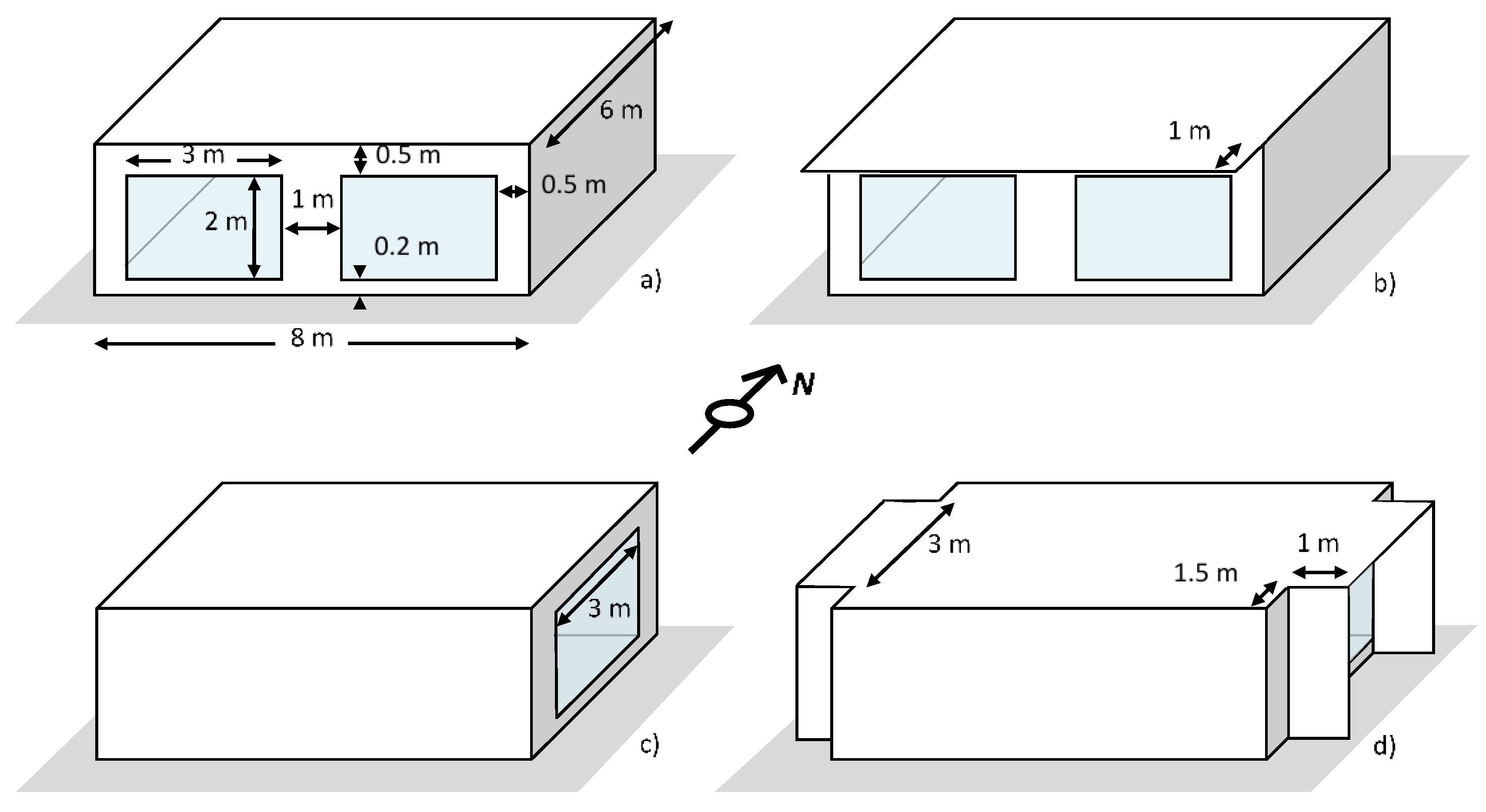
The features of the BESTEST reference building respond to a compromise between those of U.S. and European constructions. A simple rectangular plant geometry and a single thermal zone with no interior partitions are taken into account, Figure 4. Although the test cases explore different combinations of parameters and settings, the BESTEST results are related to a single annual hourly Typical Meteorological Year (TMY1) weather data file, related to the Denver, CO (USA). Its climate features a cold clear winter and a hot dry summer, with large diurnal temperature variations throughout the year. In order to check the accuracy of a simulation code under exam, for each case test the BESTEST procedure provides several results obtained by means of several codes considered as reference ones. Such programs represent, for the building energy performance analysis, the best state of the art [19]. The results provided by these reference codes delimit the reference range of the case test and the confidence interval in which the results of the simulation code under test have to be included. Note that the existence of such reference range means that no truth standard results exists in building energy performance simulations [19].

DETECt has surpassed the BESTEST reliability test. About three years were necessary for the model development and the related optimization and diagnostic processes. During such period a high number of simulations was carried out in order to satisfy the BESTEST validation procedure. In particular, by following the BESTEST diagnostic procedure and the test cases logic method [19], the algorithms or existing bugs causing discrepancies have been, step by step, fixed and eliminated. The complete code calibration was also achieved by iteratively improving the calculation procedure of some model subroutines. From this point of view, in the early version of the presented code, the divergences found between the DETECt results and the BESTEST ones were mainly due to the oversimplified handling of the solar radiation effect on the interior and exterior building surfaces. Note that through this diagnostic procedure it was possible to ungroup the particular physical effects simultaneously simulated by means of different code algorithms, detecting the related errors that in a standard simulation process could balance themselves. Moreover, such tests also allowed checking the code against itself, with the aim of analyzing the model sensitivity by varying the operating parameters taken into account in the mathematical algorithms.

4.2. BESTEST Test Cases and DETECt Assumptions

In order to definitely validate DETECt, comparisons with the mandatory BESTEST qualification cases were necessary [19]. Through such qualification cases, the DETECt reliability was checked by changing the building features and several parameters, such as direct solar gain through windows, window orientation and shadings, heating and cooling running hours, set point temperatures, building air change per hour (ACH), the set-back thermostat control.

In such tests the energy performance of a basic building envelope (Figure 4), modeled by taking into account two different inertial masses, is dealt with. Thus, two series of qualification cases are taken into consideration for the light (cases from 600 to 650) and heavyweight (cases from 900 to 950) building [19]. The BESTEST building geometry for both qualification cases 600 and 900 is a simple rectangular plant insulated room with two south facing windows. 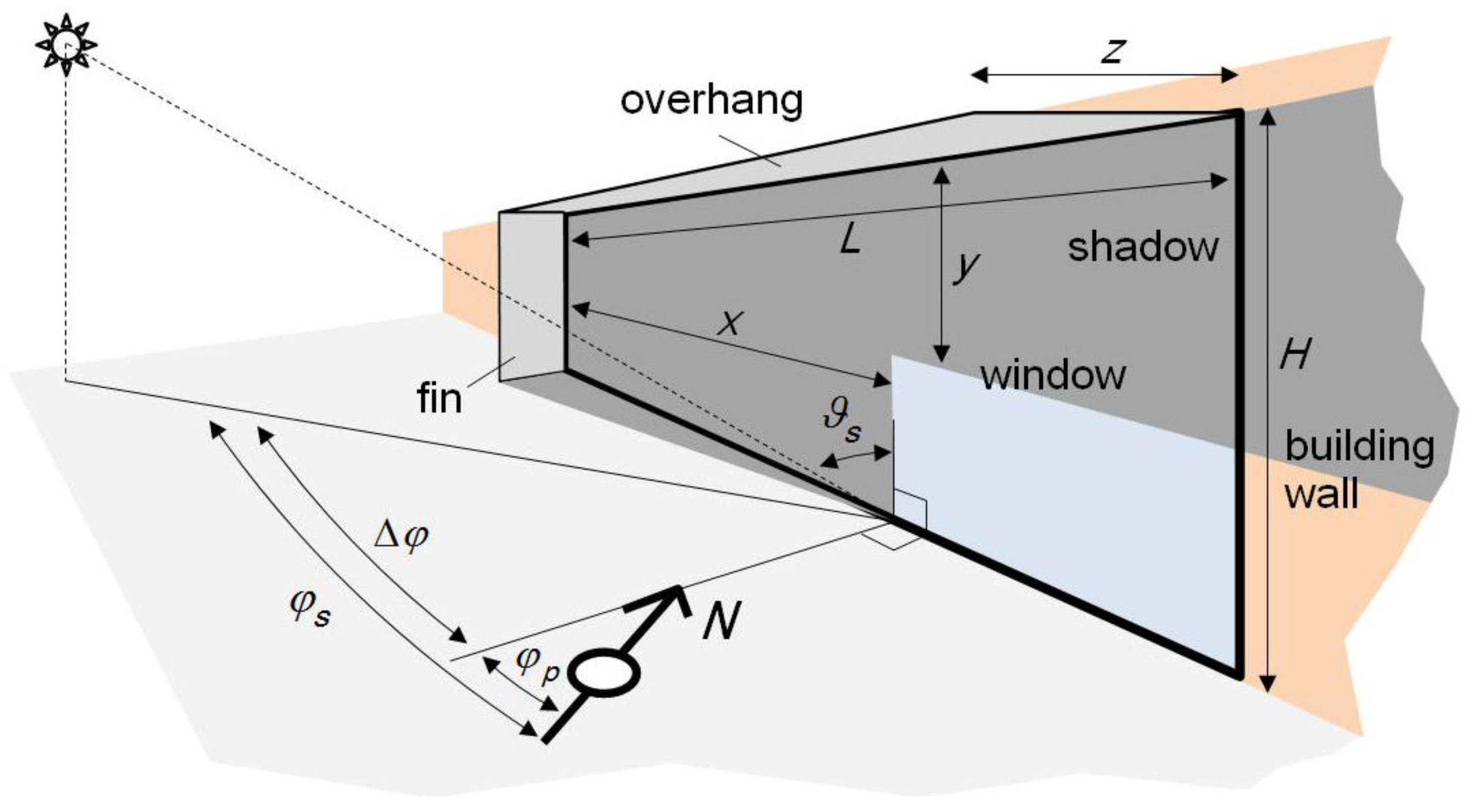All the related geometric features are shown in Figure 4a. Note that, the two south windows are considered as an equivalent single one. With respect to such cases, in cases 610 and 910 a unique horizontal overhang of 1 m width above the windows is added to the building, Figure 4b. Shifting to cases 620 and 920 the two windows are modeled on the west and east building façades, Figure 4c. With respect to such cases, in cases 630 and 930 for each window a horizontal overhang and two lateral vertical fins of 1 m width are taken into account, Figure 4d.

The thermophysical properties of the BESTEST building materials are reported in

Table 1. Thermophysical properties of the BESTEST building materials.

Materials	Conductivity, k (W/mK)	Density, d (kg/m3)	Specific heat, c (J/kgK)
Plasterboard	0.16	950	840
Fiberglas quilt	0.04	12	840
Timber flooring	0.14	650	1200
Concrete block	0.51	1400	1000
Foam insulation	0.04	10	1400
Concrete slab	1.13	1400	1000
Roofdeck/Wood siding	0.14	530	900
Glass	1.06	2500	750

. In

Table 2. BESTEST building envelope stratification (from inside to outside).

Building Element	Lightweight Building (L)		Heavyweight Building (H)
	Materials	(mm)	Materials	(mm)
Wall	Plasterboard	12	Concrete block	100
	Fiberglass quilt	66	Foam insulation	61.5
	Wood siding	9	Wood siding	9
Roof	Plasterboard	10	Identical to Lightweight case
	Fiberglass quilt	111.8
	Roof deck	19
Floor	Timber flooring	25	Concrete slab	80
	Insulation	1.003	Insulation	1.007
Window	Glass	3.2	Identical to Lightweight case

the envelope layers and the material thicknesses are reported. All the features of the mandatory qualification test cases for both light and heavy building are summarized in

Table 3. BESTEST qualification cases.

Cases	Features
Cases 600/900	Operating features: infiltration 0.5 ACH, internal sensible gain 200 W (continually), temperature set points 20 °C for heating and 27 °C for cooling (continuous regime). Geometrical data: Figure 4a
Cases 600FF/900FF	Operating features: infiltration 0.5 ACH, internal sensible gain 200 W (continually). Heating and cooling always off. Geometrical data: Figure 4a
Cases 610/910	Same operating features of cases 600/900. Geometrical data: Figure 4b
Cases 620/920	Same operating features of cases 600/900. Geometrical data: Figure 4c
Cases 630/930	Same operating features of cases 600/900. Geometrical data: Figure 4d
Cases 640/940	Same operating features of cases 600/900, except for the heating temperature set points which are here 10 °C from hours 23:00 to 7:00 and 20 °C from hours 7:00 to 23:00. Geometrical data: Figure 4a
Cases 650/950	Same operating features of cases 600/900, except for the heating and cooling strategies and the ventilation. Ventilation of 10.8 ACH from hours 18:00 to 7:00 added to infiltration. Heating always off and cooling on only from hours 7:00 to 18:00. Geometrical data: Figure 4a
Cases 650FF/950FF	Same operating features of cases 650/950. Heating and cooling always off. Geometrical data: Figure 4a
Note that FF is referred to the Free Floating regime.

. For the calculation of the window solar transmission (depending on the angle of direct solar radiation), a solar heat gain coefficient at normal incidence equal to 0.787 is taken into account. For all the mandatory BESTEST cases, the exterior and interior emissivity of the opaque surfaces are set to 0.9, while their short wave absorptance is set to 0.6. Glass infrared emissivity and absorption coefficient are set to 0.84 and 0.10, respectively. More details about such BESTEST cases are reported in [19].

The main assumptions adopted in DETECT are described. Specifically, for opaque and transparent surfaces, the internal surface unitary convection heat transfer coefficient is assumed to be equal to 3.16 W/m²·K for horizontal heat transfer on vertical surfaces and to 4.13 and 1.00 W/m²·K for upward and downward heat transfer on horizontal surfaces, respectively. The external surface unitary convection heat transfer coefficient is calculated by assuming a wind velocity of 5 m/s in case of opaque surfaces and it is set to 16.37 W/m²·K in case of windows. Note that, eventual corrections of glass surface coefficients according to window overhangs and fins are disregarded. A combined radiative and convective coefficient of the window air gap of 6.297 W/m²·K is assumed. For the investigated test cases, the DETECt simulation sample time is set to 300 s in order to obtain satisfactory dynamic building behavior and suitable system peak loads [68]. The number of nodes in which each building element is split range from 10 to 30 depending on the related weight, according to [69]. The heavier the mass element, the higher the number of nodes. Finally, in order to assure the result stability and the solution convergence, the tolerance and maximum time step solver parameters are set to 0.015 and 60 s, respectively. Here, the integration interval is set to 1 s. All the numerical DETECt results are obtained by the MatLab ode23t ODE solver [39].

4.3. Comparison with the BESTEST and Code Calibration Discussion

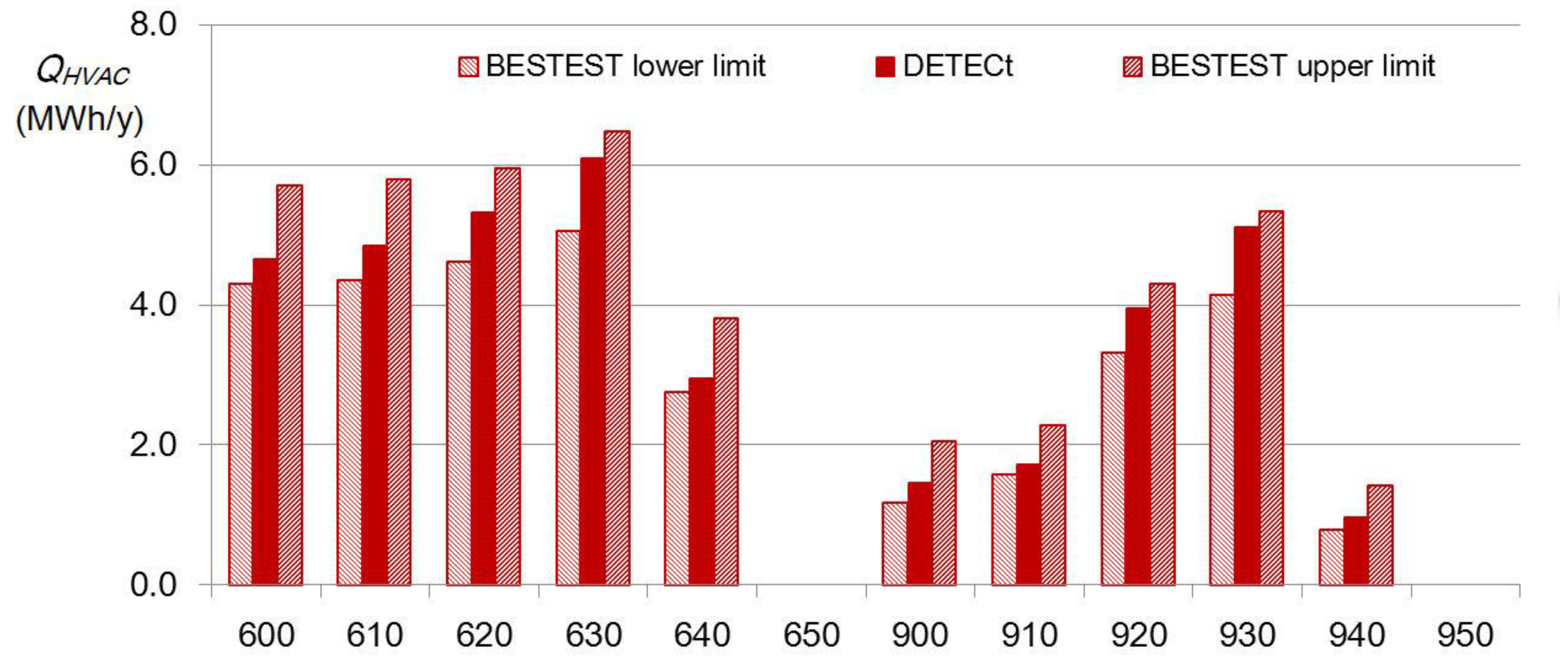
In the following, the main results obtained through the BESTEST validation procedure are summarized. Note that about thousand dynamic simulations were necessary for completing the calculation of the heating and cooling demands and temperature profiles of all the considered buildings. For all the BESTEST cases, with the exception of those in free floating regime, the comparison results related to the yearly heating and cooling energy requirements are shown in Figure 5 and Figure 6, respectively.

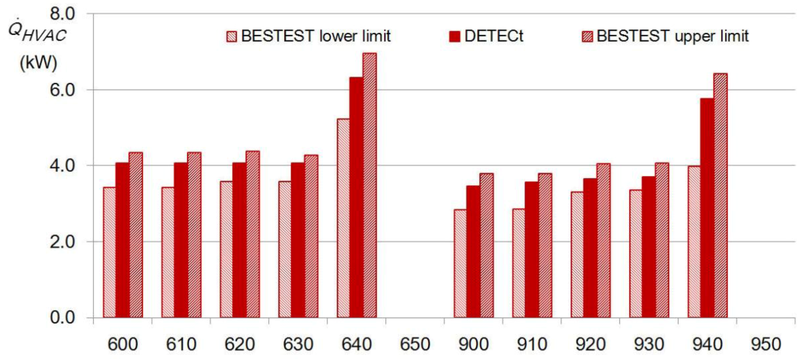
For the same cases, the obtained heating and cooling peak loads and their comparison vs. the BESTEST ones are reported in Figure 7 and Figure 8, respectively. As it is possible to observe in such figures, the differences between the results achieved by means of DETECt are always included in the confidence intervals allowed by the considered validation procedure. The BESTEST lower and upper limits reported in such figures delimit, case by case, the provided reference results ranges. The DETECt heating and cooling energy demands and loads, for all the given cases, are always included in the allowed confidence intervals.

In the following, a discussion about the refinement iterative process carried out for minimizing the sources of the detected differences, occurred during the validation tests, is reported. At the beginning of such procedures these differences were mostly due to the model algorithms related to the assessment of the solar flux absorbed by the building outside surfaces and distributed inside the indoor space. From this point of view, for the sake of simplicity, in the first versions of the presented code, no distinction between convective and radiative heat transfer on the inside and outside surfaces was assumed. Such phenomena were successively modeled through different and distinguished algorithms. In a second version of the code the solar flux transmitted by the windows toward the indoor zone was still assumed to be absorbed only by the floor. As a result of all such assumptions, an initial remarkable disagreement of the results vs. those of the reference programs was obtained. Note that, such discrepancy was detected and fixed by simulating different additional BESTEST diagnostic tests, such as case 270 (whose description and results are not reported here for the sake of brevity). Thus, in a subsequent code version, such radiation was modeled by directing it only toward the floor and partly reflecting it toward the other interior surfaces, which absorb the incoming solar radiation as a function of their absorption coefficients. Although such improvements, the long wave internal radiation was still disregarded in the model. Such simplification resulted in remarkable discrepancies particularly for the heavyweight buildings cases. In fact, the validation process showed how important is the effect of the solar gain when the building zone is characterized by thermally massive walls storing the heat gained by the absorbed solar radiation.

For these reasons, in the ultimate DETECt version, internal long wave radiation heat exchanges and multiple indoor surfaces reflections, considered as diffuse, were taken into account [70]. However, after this enhancement, both the low and high mass qualification tests for shaded cases showed light residual results differences caused by the solar radiation transmission on the east and west window surfaces. This problem was linked to the modeling of the horizontal overhang and the vertical fins located around the windows (Figure 4d), disregarding the shadow on the adjoining opaque wall surface. For the cases 630 and 930, Figure 6, the results obtained for the annual cooling requirements are close to the related minimum range bandwidth. Therefore, such results could not be linked to the disregarded estimation of the shades opaque surfaces. After several tests, such results were finally linked to the calculation of the transmitted annual solar radiation on the east and west building surfaces. For the shaded cases, such incoming radiation is resulted lower than the minimum one yielded by the reference programs,

Table 4. Annual transmitted and incident solar radiation: Results of BESTEST cases and DETECt.

Annual Transmitted Solar Radiation (kWh/m2·year)		Min BESTEST	DETECt	Max BESTEST
620/920 West	Unshaded	563	620	735
600/900 South		914	1032	1051
630/930 West	Shaded	431	412	599
610/910 South		757	812	831
Annual Incident Solar Radiation (kWh/m2·year)		Min BESTEST	DETECt	Max BESTEST
North		367	399	457
East		959	1096	1217
West		857	896	1090
South		1456	1479	1566
Horizontal		1797	1832	1832

. Here, for the unshaded test cases, the annual transmitted solar radiations (diffuse and direct) through west- and south-facing windows (concerning cases 620 (or 920) and 600 (or 900), respectively) are reported.

In the same table, for the same oriented surfaces, the diffuse and direct shaded annual transmitted solar radiations (concerning cases 630 (or 930) and 610 (or 910)) are also shown. Note that, concerning the transmitted solar radiation, such good agreements have been obtained by means of a variable direct shortwave transmission coefficient of windows. This, in the first version of the code, was kept constant without accounting for the hourly sunlight incident angle dependence. In Table 4 the annual incident solar radiations on all the vertical and horizontal surfaces are also reported. In this table a good agreement among the DETECt results and those provided by the BESTEST procedure is always achieved.

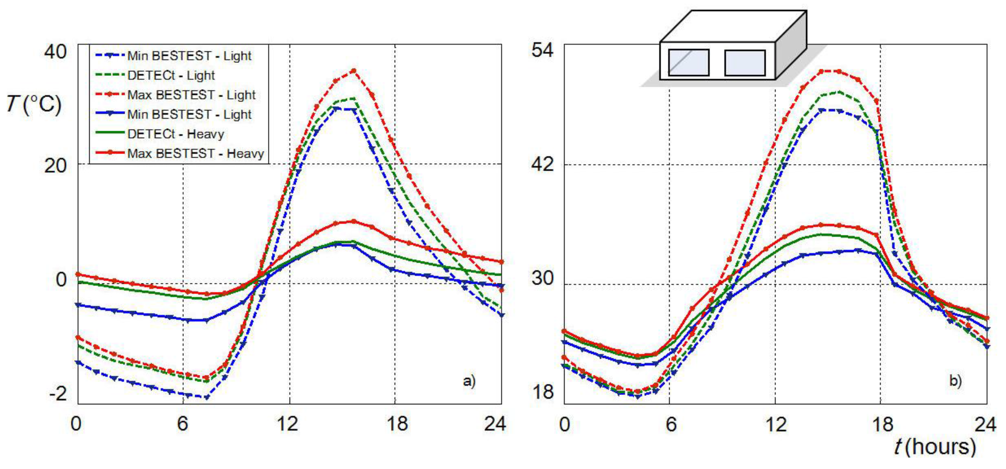
As written above, the BESTEST validation procedure requires the assessment of some hourly variables and their comparison vs. the reference trends [19]. In particular, the calculated hourly free floating temperatures trends and their annual minimum and maximum values must to be checked. From this point of view, in

Table 5. Annual hourly zone temperatures reported for BESTEST cases and obtained through DETECt.

Cases	Minimum Temperature (°C)			Maximum Temperature (°C)			Average Temperature (°C)
	Min BESTEST	DETECt	Max BESTEST	Min BESTEST	DETECt	Max BESTEST	Min BESTEST	DETECt	Max BESTEST
600FF	−18.80	−16.20	−15.57	64.90	68.50	69.50	24.22	25.20	25.93
900FF	−6.38	−2.10	−1.65	41.81	43.90	44.80	24.45	25.50	25.93
650FF	−23.00	−21.30	−21.60	63.24	67.50	68.20	17.99	18.50	19.62
950FF	−20.20	−18.20	−18.60	35.54	37.50	38.50	14.00	14.20	14.97

the annual minimum and maximum temperatures for the free floating cases (cases 600FF/900FF and 650FF/950FF) are reported. In this table, it is possible to observe that almost all the DETECt results are included in the BESTEST allowed ranges. For the same cases, the comparison vs. the BESTEST data of the simulated free floating temperatures trends are reported for the winter day, selected for the BESTEST procedure, in Figure 9a and for the summer one in Figure 9b. Here, the calculated profiles are resulted always included between the minimum and maximum reference ones. 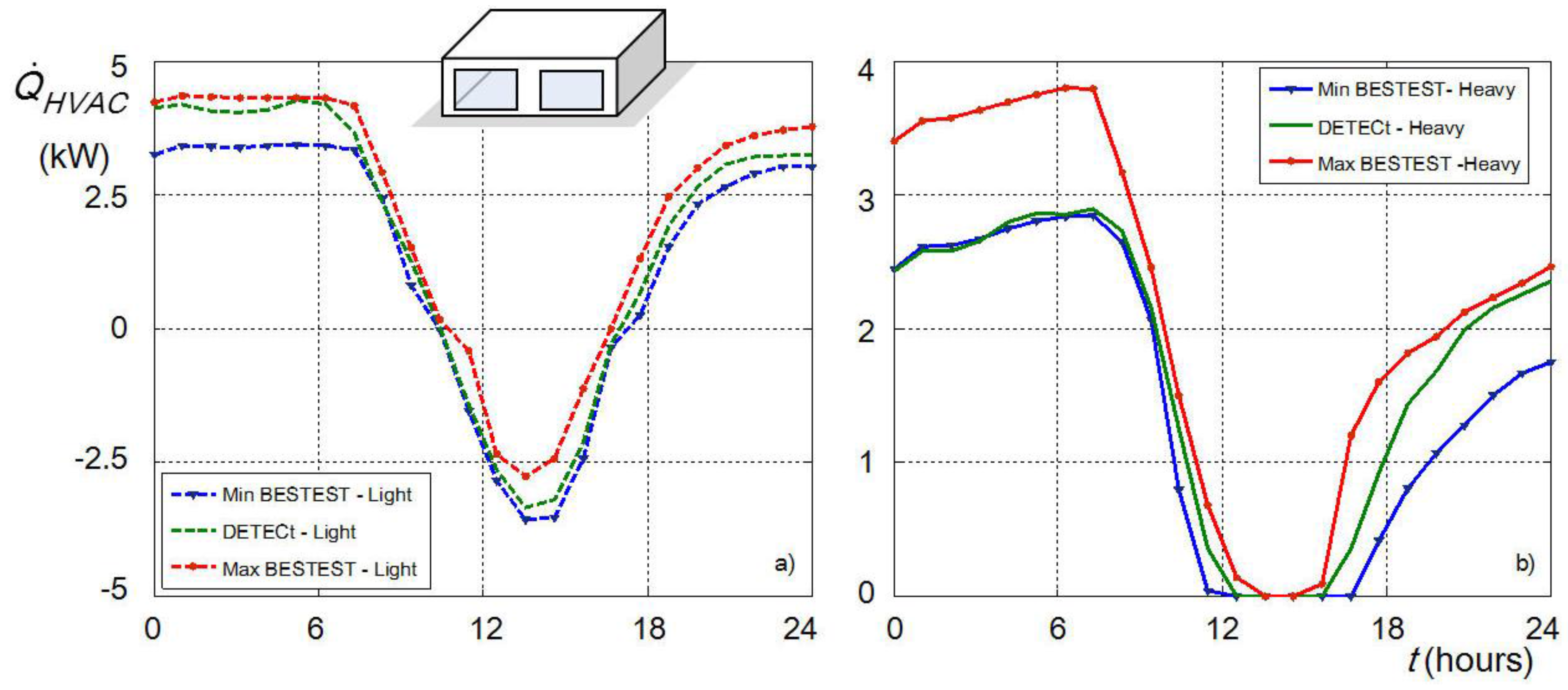In Figure 10a for case 600 and in Figure 10b for case 900 the heating and cooling requirements are reported for the winter day selected by the BESTEST procedure. Also in this case the calculated profiles are always included between the minimum and maximum reference ones.

Note that, according to the BESTEST results no cooling energy demand is required by the heavyweight building, Figure 10b. This is also due to the considered cooling set point (27 °C, Table 3). Comparing the calculated free floating temperature trend (Figure 9a) to the heating and cooling requirements one of the same winter day (Figure 10a), it is possible to observe that only for the lightweight case no correspondence between the related hourly values is obtained. In fact, to the calculated temperature close to the reference upper limit should correspond a calculated heating energy requirement close to the reference lower limit.

Such an outcome, probably due to the adopted thermostat controller, was also noted in the results achieved by some BESTEST reference programs. Since the calculated hourly energy requirements and temperature trends for the considered days, reported in Figure 9 and Figure 10, agree well with the reference results, concerning the remaining results no additional problems regarding the thermal dynamics (as well as the thermostat controller) can be observed.

5. Outputs

In the following some examples about the potentiality of the presented code are reported. In particular, for some of the above described test cases the time history and the spatial trends of some thermophysical properties useful in a building energy analysis are reported.

In Figure 11, Figure 12, Figure 13, Figure 14 and Figure 15 some dynamic outputs obtained through DETECt are reported. By means of such a graphical tool the main thermal phenomena occurring in an investigated building can be detected. In addition, design and operating guidelines can be easily obtained through each energy performance simulation. 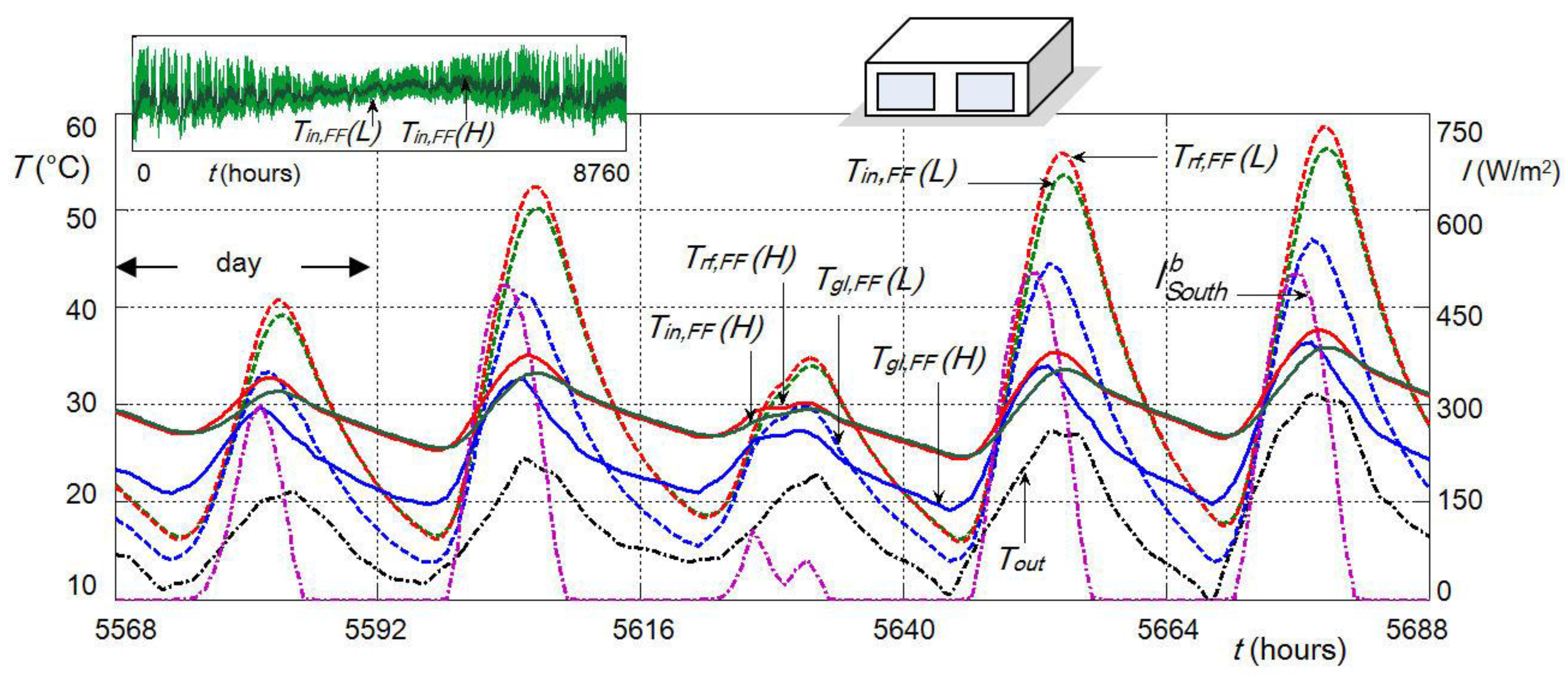In particular, in Figure 11 for the test cases 600 (L: lightweight) and 900 (H: heavyweight), by switching off the HVAC system (free floating, FF, regime), the dynamic trends of the indoor air temperature (T_in,FF), the internal surfaces temperatures of the window glass (T_gl,FF) and the roof (T_rf,FF) are depicted for several summer days (August 21st–25th).

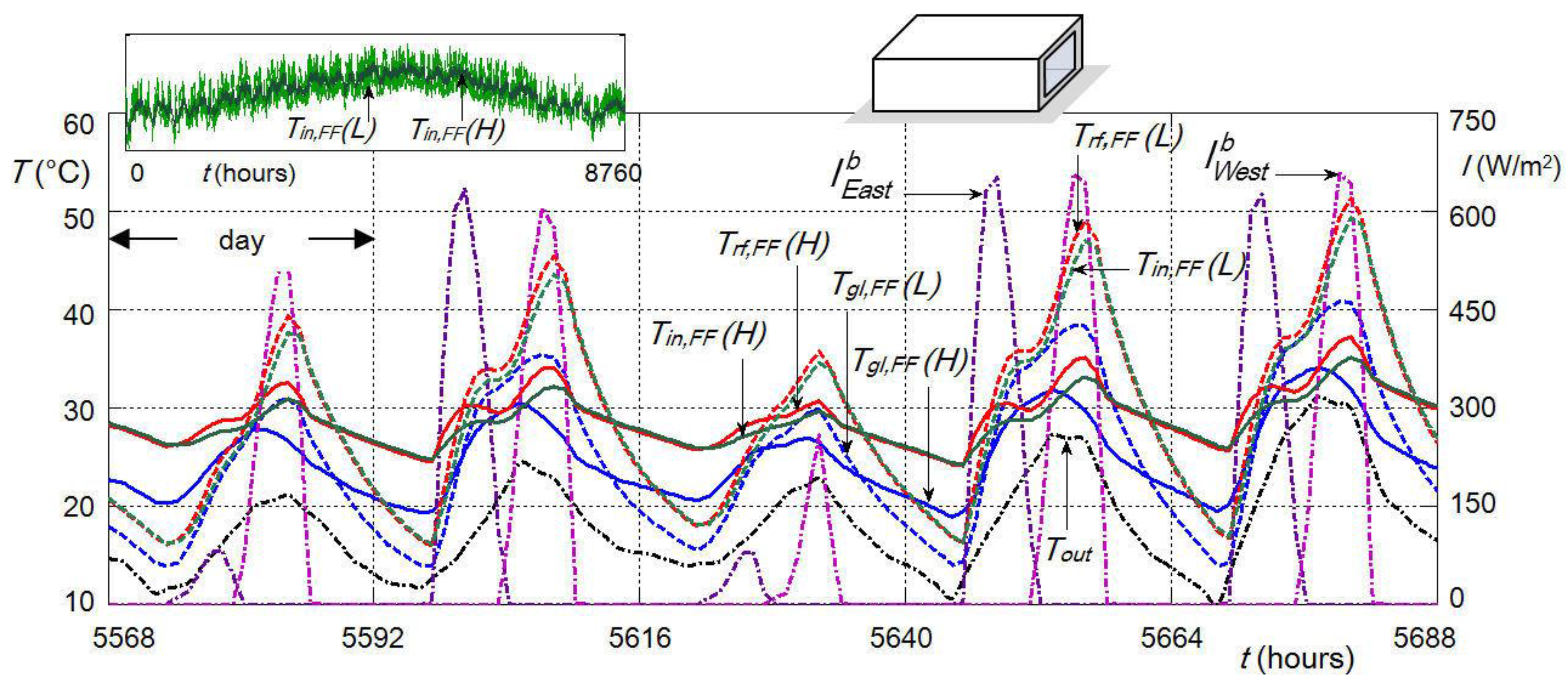
In Figure 12 for the same summer days and the same internal surfaces and indoor air temperatures of Figure 11, the dynamic profiles of the free floating regime are depicted for the test cases 620 (L: lightweight) and 920 (H: heavyweight). In the same graphs the profiles of the outdoor air temperature (T_out) and of the beam solar radiations incident on the south vertical wall ($I_{South}^b$), Figure 11, and on the east and west vertical walls ($I_{East}^b$ and $I_{West}^b$), Figure 12 are also shown. In the high left side of these figures the yearly dynamic trends T_in,FF, for both light and heavyweight envelopes, are also reported. Note that, in the case of free floating regime, the thermal fluxes through walls are directed from inside to outside, most of the time. In Figure 11 and Figure 12 the thermal inertia effect of the building envelopes can be observed by means of the peaks of T_in and T_rf, which are always delayed with respect to the T_gl ones. In Figure 11, the T_gl are obviously the closest to the peaks of $I_{South}^b$. Note that for the lightweight envelopes, higher interior and indoor temperature are always achieved by the building with facing south windows vs. that one with windows located on the east and west façades. Obviously, the indoor air temperature fluctuation during the whole day is more remarkable for the lightweight envelope building. Note also that, without switching on the HVAC system, during the daytime the indoor air temperatures are far (H: heavyweight) or very far (L: lightweight) from the comfort ones (T_in,FF always higher than 27 °C). During the night time, such occurrence is detected only for the lightweight envelope building (T_in,FF lower than 20 °C). In the investigated summer days, for both the envelope cases the indoor air temperature is always much higher than the outdoor one. At last, by means of such graphical tools the average radiant temperature of the investigated thermal zone can be easily assessed.

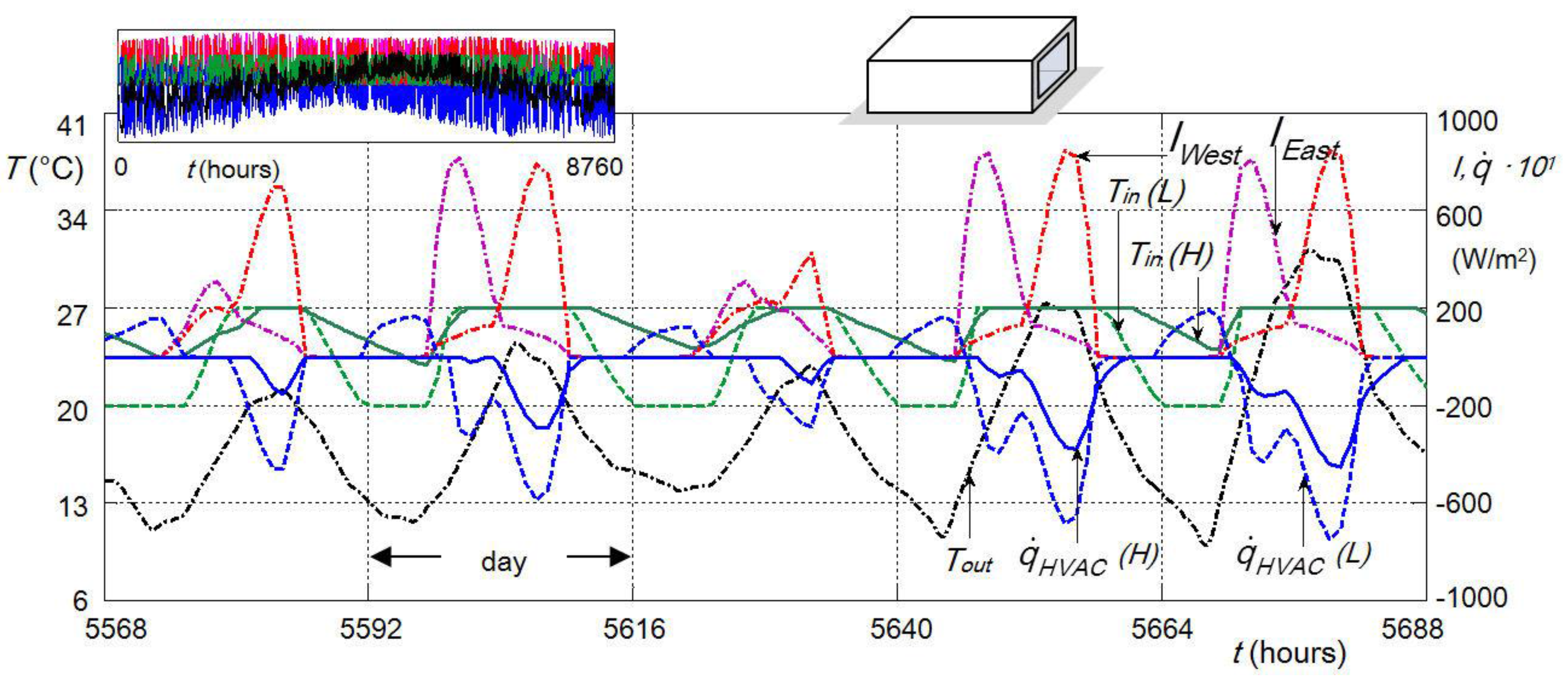
In Figure 13 and Figure 14, in case of switched on HVAC system, for both the light (L) and heavy (H) envelopes of test cases 600/900 and 620/920, the temperature dynamic trends of indoor air (T_in) are shown. Such profiles are referred to the HVAC system activation beyond the set point temperatures of 20 and 27 °C for the same previously accounted summer days of the FF regime figures.

In the same figures, the profiles of T_out and of the total solar radiations on vertical south ($I_{South}$), Figure 13, and east and west ($I_{East}$ and $I_{West}$), Figure 14, external surfaces of the buildings are also reported. The dynamic trends of the related sensible cooling heat flux (${\dot{q}}_{HVAC}$) are shown too. In the high left side of such figures the dynamic profiles of all these parameters are reported for the whole year. ${\dot{q}}_{HVAC}$ is obviously accounted during the T_in control, which continually occurs for the whole day. Note that the cooling energy demand is higher for the lightweight envelope building and the heating load is obtained only for the lightweight one. The short time lag between ${\dot{q}}_{HVAC}$(L) and ${\dot{q}}_{HVAC}$(H) is due to the global low envelope weight difference. Note that the light and heavy wall (floor) weights are 17 and 145 kg/m² (26 and 122 kg/m²), respectively, whereas the same roof weight of about 21 kg/m² is simulated for both the light and heavy envelopes.

In Figure 15 on the left side for cases 600FF and 900FF, respectively, the dynamic profiles of the simulated internal and external roof surfaces, T_rf,int and T_rf,ext, respectively, and the dynamic profiles of the indoor air, T_in, temperatures obtained through DETECt and a reference simulation code, REF, are reported for a summer day (June 12th). In the same figures the T_out profile is also depicted. Here, as reference software, for comparison purposes, was assumed TRNSYS 17, considered as a BEPS tool well representative of the recent state of the art. Note that, the results of the BESTEST cases achieved by using such newer tool version can show significant differences vs. the original previous one included in the BESTEST procedure. This is due to the code improvement (as consequence of the remarkable developments in building sciences and technologies achieved from 1980s) and to the user interpretations of standards and simulation assumptions during the BESTEST cases reproduction [71]. Concerning the comparison between DETECt and REF dynamic profiles, a good agreement is observed. The reference software seems to slightly underestimate the T_in assessment. In particular, it was verified that the calculated heating and cooling demands and peaks obtained through TRNSYS 17 for the BESTEST cases 600 and 900, differ from those calculated by means of previous TRNSYS versions [72]. In addition, whereas the heating requirements obtained through TRNSYS 17 still comfortably fall within the reference present BESTEST acceptability ranges, the cooling ones slightly fall below the correspondent confidence lower limits. At the right side of Figure 15 the spatial temperature gradients across the roof stratification are reported for some time intervals of the day and for both light and heavyweight envelopes. On the x-axis of such graphs the considered thickness between the interior and exterior surfaces is reported. It must be noted that for both light and heavyweight buildings, the material and thickness of the roof layers are the same. Here, an incoming heat flux through such building component is detected for most of the time. In particular, although the very short time lag between indoor air temperatures of light and heavyweight envelopes, an outgoing heat flux from the building through the roof occurs only from 7:00 to 13:00 for case 600FF and only from 12:00 to 17:00 for case 900FF. Note that higher temperature gradients are obtained across the central insulation layer, as expected.

6. Conclusions

In this paper the main features of a dynamic building energy performance simulation model, purposely developed for research purposes [25], are described. The building simulation model, called DETECt, is capable of predicting the dynamic thermos-hygrometric behavior of mono- and multi-zone, as well multi-story buildings and assessing the benefits of different and advanced building envelope integrated techniques (e.g., building integrated solar thermal systems, phase change materials, etc.), solar gain controls and advanced daylighting strategies in case of different weather locations, envelope materials, building shapes, orientations and geometries. The code is also able to carry out suitable parametric analyses, which can be easily performed through a single iterative simulation run, without the need of re-entering, step by step, the building models and the features to be varied.

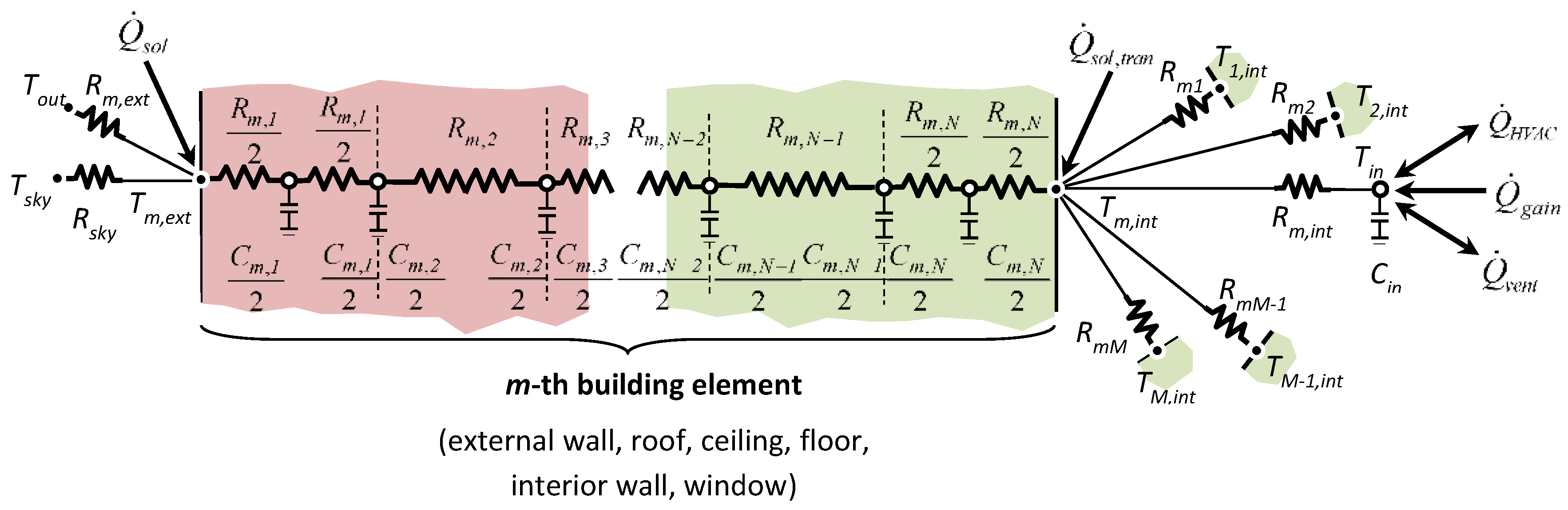
The steps and results of the validation procedure, based on the BESTEST, carefully followed to validate the presented dynamic simulation model, are here described. A brief description of the mathematical models and algorithms are also reported in order to provide insights about the engine logic and to show the model assumptions that primarily influence the fidelity and accuracy of the simulation results. Specifically, the physical building model implemented in DETECt is based on a high order resistive-capacitive (RC) thermal network obtained through distributed parameters. Capabilities and outputs of the code, including few application examples, are finally presented.

DETECt exceeded the carried out validation procedure. The simulation results obtained through DETECt, compared to those provided by the BESTEST, are always included within the provided confidence intervals. In order to show the potentiality of the simulation code, the most important outputs referred to different BESTEST cases are reported and suitably discussed. They refer to heating and cooling demands, calculated over the whole year or a selected time horizon, heating and cooling loads, temperatures of indoor air, building elements surfaces and nodes.

DETECt allows one to carry out comprehensive and whole building energy performance and comfort analyses, by properly taking into account the passive and active effects due to the building integration of innovative building integrated technologies, such as BIPVT-BISTS, PCM, etc. [28]. The code also includes a graphical tool for plotting the dynamic profiles of building temperatures and heat fluxes and the time-variant spatial trend of temperature in the building elements. DETECt can be also linked to other additional computer subroutines for the performance simulation of building plant systems also supported by innovative and renewable energy technologies. Thanks to the code, any innovative technology can be implemented within the simulation code, depending on the occurring research needs. Finally, with the help of all the results obtained through the presented code, useful guidelines for the energy design of new buildings (such as NZEBs) or for the energy refurbishment of the existing ones can be obtained.

References

1. Transition to Sustainable Buildings. Strategies and Opportunities to 2050; International Energy Agency (IEA): Paris, France, 2013.
2. Negendahl, K. Building performance simulation in the early design stage: An introduction to integrated dynamic models. Autom. Constr. 2015, 54, 39–53. [Google Scholar] [CrossRef]
3. Szalay, Z.; Zöld, A. Definition of nearly zero-energy building requirements based on a large building sample. Energy Policy 2014, 74, 510–521. [Google Scholar] [CrossRef]
4. Nembrini, J.; Samberger, S.; Labelle, G. Parametric scripting for early design performance simulation. Energy Build. 2014, 68, 786–798. [Google Scholar] [CrossRef]
5. Todorović, M.S. BPS, energy efficiency and renewable energy sources for buildings greening and zero energy cities planning: Harmony and ethics of sustainability. Energy Build. 2012, 48, 180–189. [Google Scholar] [CrossRef]
6. Directive 2010/31/EU of the European Parliament and of the Council on the Energy Performance of Buildings (Recast); European Parliament: Strasbourg, France, 2010.
7. Diakaki, C.; Grigoroudis, E.; Kolokotsa, D. Towards a multi-objective optimization approach for improving energy efficiency in buildings. Energy Build. 2008, 40, 1747–1754. [Google Scholar] [CrossRef]
8. Fumo, N. A review on the basics of building energy estimation. Renew. Sustain. Energy Rev. 2014, 31, 53–60. [Google Scholar] [CrossRef]
9. Bigot, D.; Miranville, F.; Fakra, A.H.; Boyer, H. A nodal thermal model for photovoltaic systems: Impact on building temperature fields and elements of validation for tropical and humid climatic conditions. Energy Build. 2009, 41, 1117–1126. [Google Scholar] [CrossRef]
10. Bigot, D.; Miranville, F.; Boyer, H.; Bojic, M.; Guichard, S.; Jean, A. Model optimization and validation with experimental data using the case study of a building equipped with photovoltaic panel on roof: Coupling of the building thermal simulation code ISOLAB with the generic optimization program GenOpt. Energy Build. 2013, 58, 333–347. [Google Scholar] [CrossRef]
11. Guichard, S.; Miranville, F.; Bigot, D.; Boyer, H. A thermal model for phase change materials in a building roof for a tropical and humid climate: Model description and elements of validation. Energy Build. 2014, 70, 71–80. [Google Scholar] [CrossRef]
12. Clarke, J.A.; Hensen, J.L.M. Integrated building performance simulation: Progress, prospects and requirements. Build. Environ. 2015, 91, 294–306. [Google Scholar] [CrossRef]
13. Crawley, D.B.; Hand, J.W.; Kummert, M.; Griffith, B.T. Contrasting the capabilities of building energy performance simulation programs. Part Spec. Build. Perform. Simul. 2008, 43, 661–673. [Google Scholar] [CrossRef] [Green Version]
14. Attia, S.; Gratia, E.; De Herde, A.; Hensen, J.L.M. Simulation-based decision support tool for early stages of zero-energy building design. Energy Build. 2012, 49, 2–15. [Google Scholar] [CrossRef]
15. Fonseca i Casas, P.; Fonseca i Casas, A.; Garrido-Soriano, N.; Casanovas, J. Formal simulation model to optimize building sustainability. Adv. Eng. Softw. 2014, 69, 62–74. [Google Scholar] [CrossRef] [Green Version]
16. Ben-Nakhi, A.E.; Aasem, E.O. Development and integration of a user friendly validation module within whole building dynamic simulation. Energy Convers. Manag. 2003, 44, 53–64. [Google Scholar] [CrossRef]
17. Attia, S. State of the Art of Existing Early Design Simulation Tools for Net Zero Energy Buildings: A Comparison of Ten Tools; Université Catholique de Louvain: Brussels, Belgium, 2011. [Google Scholar]
18. IEA—SHC. Annex 43/SHC Task 34: Testing and Validation of Building Energy Simulation Tools. Available online: http://vbn.aau.dk/en/projects/iea--shc-task-34ecbcs-annex-43-testing-and-validation-of-building-energy-simulation-tools%289bb9c4fa-125d-494c-8e9d-ca4806582a8a%29.html (accessed on 18 April 2016).
19. Judkoff, R.; Neymark, J. International Energy Agency Building Energy Simulation Test (BESTEST) and Diagnostic Method, NREL/TP-472-6231; National Renewable Energy Laboratory (NREL): Golden, CO, USA, 2005. [Google Scholar]
20. ASHRAE. Available online: http://sspc140.ashraepcs.org/ (accessed on 18 April 2016).
21. EN ISO 13791:2012—Thermal Performance of Buildings—Calculation of Internal Temperatures of a Room in Summer Without Mechanical Cooling—General Criteria and Validation Procedures; CEN European Committee for Standardization: Brussels, Belgium, 2012.
22. Joudi, A.; Svedung, H.; Rönnelid, M. Energy efficient surfaces on building sandwich panels—A dynamic simulation model. Energy Build. 2011, 43, 2462–2467. [Google Scholar] [CrossRef]
23. Transient System Simulation Tool, TRNSYS. Available online: http://www.trnsys.com (accessed on 18 April 2016).
24. Ramallo-González, A.P.; Eames, M.E.; Coley, D.A. Lumped parameter models for building thermal modelling: An analytic approach to simplifying complex multi-layered constructions. Energy Build. 2013, 60, 174–184. [Google Scholar] [CrossRef] [Green Version]
25. Buonomano, A.; Palombo, A. Building energy performance analysis by an in-house developed dynamic simulation code: An investigation for different case studies. Appl. Energy 2014, 113, 788–807. [Google Scholar] [CrossRef]
26. Sahlin, P.; Eriksson, L.; Grozman, P.; Johnsson, H.; Shapovalov, A.; Vuolle, M. Whole-building simulation with symbolic DAE equations and general purpose solvers. Build. Environ. 2004, 39, 949–958. [Google Scholar] [CrossRef]
27. Buonomano, A.; Montanaro, U.; Palombo, A.; Santini, S. Dynamic building energy performance analysis: A new adaptive control strategy for stringent thermohygrometric indoor air requirements. Appl. Energy 2016, 163, 361–386. [Google Scholar] [CrossRef]
28. Buonomano, A.; De Luca, G.; Montanaro, U.; Palombo, A. Innovative technologies for NZEBs: An energy and economic analysis tool and a case study of a non-residential building for the Mediterranean climate. Energy Build. 2015. [Google Scholar] [CrossRef]
29. Buonomano, A.; Calise, F.; Palombo, A. Solar heating and cooling systems by CPVT and ET solar collectors: A novel transient simulation model. Appl. Energy 2013, 103, 588–606. [Google Scholar] [CrossRef]
30. Al-Homoud, M.S. Computer-aided building energy analysis techniques. Build. Environ. 2001, 36, 421–433. [Google Scholar] [CrossRef]
31. Xu, X.; Wang, S. A simplified dynamic model for existing buildings using CTF and thermal network models. Int. J. Therm. Sci. 2008, 47, 1249–1262. [Google Scholar] [CrossRef]
32. Lombard, C.; Mathews, E.H. A two-port envelope model for building heat transfer. Build. Environ. 1998, 34, 19–30. [Google Scholar] [CrossRef]
33. Pisello, A.L.; Goretti, M.; Cotana, F. A method for assessing buildings’ energy efficiency by dynamic simulation and experimental activity. Appl. Energy 2012, 97, 419–429. [Google Scholar] [CrossRef]
34. Kontoleon, K.J. Dynamic thermal circuit modelling with distribution of internal solar radiation on varying façade orientations. Energy Build. 2012, 47, 139–150. [Google Scholar] [CrossRef]
35. VanderVeken, J.; Saelens, D.; Verbeeck, G.; Hens, H. Comparison of steady-state and dynamic building energy simulation programs. In Proceedings of the Internation Buildings IX ASHRAE Conference on the Performance of Exterior Envelopes of Whole Buildings, Clearwater Beach, FL, USA, 5–10 December 2004.
36. Maile, T.; Fischer, M.; Haymaker, J.; Bazjanac, V. Formalizing Approximations, Assumptions, and Simplifications to Document Limitations in Building Energy Performance Simulation; CIFE Working Paper; Stanford University: Stanford, CA, USA, 2010. [Google Scholar]
37. Martin, K.; Erkoreka, A.; Flores, I.; Odriozola, M.; Sala, J.M. Problems in the calculation of thermal bridges in dynamic conditions. Energy Build. 2011, 43, 529–535. [Google Scholar] [CrossRef]
38. Tsilingiris, P.T. Parametric space distribution effects of wall heat capacity and thermal resistance on the dynamic thermal behavior of walls and structures. Energy Build. 2006, 38, 1200–1211. [Google Scholar] [CrossRef]
39. Mathworks. MatLab. Available online: http://www.mathworks.com (accessed on 18 April 2016).
40. Buonomano, A.; Calise, F.; Palombo, A. Buildings dynamic simulation: Water loop heat pump systems analysis for European climates. Appl. Energy 2012, 91, 222–234. [Google Scholar] [CrossRef]
41. Tsilingiris, P.T. Wall heat loss from intermittently conditioned spaces—The dynamic influence of structural and operational parameters. Energy Build. 2006, 38, 1022–1031. [Google Scholar] [CrossRef]
42. Paris, B.; Eynard, J.; Grieu, S.; Talbert, T.; Polit, M. Heating control schemes for energy management in buildings. Energy Build. 2010, 42, 1908–1917. [Google Scholar] [CrossRef]
43. ASHRAE. ASHRAE handbook, Fundamentals—Chapter 7. In American Society of Heating Refrigerating and Air-Conditioning Engineers; ASHRAE: Atlanta, GA, USA, 2009. [Google Scholar]
44. Zhou, J.Q.; Claridge, D.E. PI tuning and robustness analysis for air handler discharge air temperature control. Energy Build. 2012, 44, 1–6. [Google Scholar] [CrossRef]
45. Kreider, J.F.; Rabl, A. Heating and Cooling of Buildings; McGraw-Hill: New York, NY, USA, 2009. [Google Scholar]
46. Bergman, T.L.; Lavine, A.S.; Incropera, F.P.; Dewit, P.D. Fundamentals of Heat and Mass Transfer, 7th ed.; John Wiley & Sons: New York, NY, USA, 2011. [Google Scholar]
47. Gebhart, B. A new method for calculating radiant exchanges. ASHRAE Trans. 1959, 92, 95–104. [Google Scholar]
48. Mottard, J.-M.; Fissore, A. Thermal simulation of an attached sunspace and its experimental validation. Solar Energy 2007, 81, 305–315. [Google Scholar] [CrossRef]
49. Buonomano, A.; Montanaro, U.; Palombo, A.; Santini, S. Adaptive control for building thermo-hygrometric analysis: A novel dynamic simulation code for indoor spaces with multi-enclosed thermal zones. Energy Proced. 2015, 78, 2190–2195. [Google Scholar] [CrossRef]
50. Oliveira Pañao, M.J.N.; Santos, C.A.P.; Mateus, N.M.; Graca, G.C. Validation of a lumped RC model for thermal simulation of a doubleskin natural and mechanical ventilated test cell. Energy Build. 2016, 121, 92–103. [Google Scholar]
51. Liu, M.; Wittchen, K.B.; Heiselberg, P.K.; Winther, F.V. Development and sensitivity study of a simplified and dynamic method for double glazing facade and verified by a full-scale façade element. Energy Build. 2014, 68, 432–443. [Google Scholar] [CrossRef]
52. Goia, F.; Perino, M.; Haase, M. A numerical model to evaluate the thermal behaviour of PCM glazing system configurations. Energy Build. 2012, 54, 141–153. [Google Scholar] [CrossRef]
53. Pantic, S.; Candanedo, L.; Athienitis, A.K. Modeling of energy performance of a house with three configurations of building-integrated photovoltaic/thermal systems. Energy Build. 2010, 42, 1779–1789. [Google Scholar] [CrossRef]
54. Pisello, A.; Bobker, M.; Cotana, F. A building energy efficiency optimization method by evaluating the effective thermal zones occupancy. Energies 2012, 5, 5257–5278. [Google Scholar] [CrossRef]
55. Soares, N.; Costa, J.J.; Gaspar, A.R.; Santos, P. Review of passive PCM latent heat thermal energy storage systems towards buildings’ energy efficiency. Energy Build. 2013, 59, 82–103. [Google Scholar] [CrossRef]
56. Heier, J.; Bales, C.; Martin, V. Combining thermal energy storage with buildings—A review. Renew. Sustain. Energy Rev. 2015, 42, 1305–1325. [Google Scholar] [CrossRef]
57. Overview of BISTS State of the Art, Models and Applications; COST Action TU1205 (BISTS); Cyprus University of Technology: Lymassol, Cyprus, 2015; ISBN 978-9963-697-16-8.
58. Ma, T.; Yang, H.; Zhang, Y.; Lu, L.; Wang, X. Using phase change materials in photovoltaic systems for thermal regulation and electrical efficiency improvement: A review and outlook. Renew. Sustain. Energy Rev. 2015, 43, 1273–1284. [Google Scholar] [CrossRef]
59. Li, X.; Wen, J. Review of building energy modeling for control and operation. Renew. Sustain Energy Rev. 2014, 37, 517–537. [Google Scholar] [CrossRef]
60. Antonopoulos, K.A.; Koronaki, E.P. On the dynamic thermal behaviour of indoor spaces. Appl. Therm. Eng. 2001, 21, 929–940. [Google Scholar] [CrossRef]
61. Pomianowski, M.; Heiselberg, P.; Zhang, Y. Review of thermal energy storage technologies based on PCM application in buildings. Energy Build. 2013, 67, 56–69. [Google Scholar] [CrossRef]
62. Building Components and Building Elements—Thermal Resistance and Thermal Transmittance—Calculation Method; ISO 6946:2008; ISO International Organization for Standardization: Geneva, Switzerland, 2008.
63. Ryan, M.R.; Sanquist, T.F. Validation of building energy modeling tools under idealized and realist conditions. Energy Build. 2012, 47, 375–382. [Google Scholar] [CrossRef]
64. Judkoffm, R.; Wortmanm, D.; O’Doherty, B.; Burch, J. A Methodology for validating Building Energy Analysis Simulations; SERI/TR-254-1508; Solar Energy Research Institute (now National Renewable Energy Laboratory): Golden, CO, USA, 1983. [Google Scholar]
65. Neymark, J.; Judkoff, R.; Knabe, G.; Le, H.-T.; Durig, M.; Glass, A.; Zweifel, G. Applying the building energy simulation test (BESTEST) diagnostic method to verification of space conditioning equipment models used in whole-building energy simulation programs. Energy Build. 2002, 34, 917–931. [Google Scholar] [CrossRef]
66. EN 15265:2007—Thermal Performance of Buildings—Calculation of Energy Use for Space Heating and Cooling—General Criteria and Validation Procedures; CEN European Committee for Standardization: Brussels, Belgium, 2007.
67. ANSI/ASHRAE Standard 90.1–2004: Energy Standard for Building Except Low-Rise Residential Buildings; ASHRAE American Society of Heating Refrigerating and Air-Conditioning Engineers: Atlanta, GA, USA, 2004.
68. Ghiaus, C.; Hazyuk, I. Calculation of optimal thermal load of intermittently heated buildings. Energy Build. 2010, 42, 1248–1258. [Google Scholar] [CrossRef]
69. Freire, R.Z.; Mazuroski, W.; Abadie, M.O.; Mendes, N. Capacitive effect on the heat transfer through building glazing systems. Appl. Energy 2011, 88, 4310–4319. [Google Scholar] [CrossRef]
70. Chatziangelidis, K.; Bouris, D. Calculation of the distribution of incoming solar radiation in enclosures. Appl. Therm. Eng. 2010, 29, 1096–1105. [Google Scholar] [CrossRef]
71. Bradley, D.E.; Kummert, M.; McDowell, T.P. Experiences with and interpretation of standard test methods of building energy analysis tools. In Proceedings of the IBPSA-Canada Bi-Annual Conference, Vancouver, BC, Canada, 9–11 June 2004.
72. Aschaber, J.; Hiller, M.; Weber, R. TRNSYS17: New features of the multizone building model. In Proceedings of the Eleventh International IBPSA Conference, Glasgow, Scotland, UK, 27–30 July 2009.
Figure 1. Simulator scheme and concept.
Energies 09 00301 g001
Figure 2. Schematics of the resistance capacitance (RC) thermal network.
Energies 09 00301 g002
Figure 3. South facing window shaded by a horizontal overhang and a vertical fin.
Energies 09 00301 g003
Figure 4. BESTEST buildings: (a) Cases 600/900; (b) Cases 610/910; (c) Cases 620/920; (d) Cases 630/930.
Energies 09 00301 g004
Figure 5. Heating annual energy demand for light and heavyweight building qualification tests.
Energies 09 00301 g005
Figure 6. Cooling annual energy demand for light and heavyweight building qualification tests.
Energies 09 00301 g006
Figure 7. Heating integrated peak for light and heavyweight building qualification tests.
Energies 09 00301 g007
Figure 8. Cooling integrated peak for light and heavyweight building qualification tests.
Energies 09 00301 g008
Figure 9. Hourly free floating temperature: (a) January 4th (cases 600/900 FF), (b) July 27th (cases 650/950 FF).
Energies 09 00301 g009
Figure 10. Hourly heating and cooling loads: (a) Case 600, (b) Case 900—January 4th.
Energies 09 00301 g010
Figure 11. BESTEST cases 600 and 900 by switched off HVAC system (Free Floating profiles): DETECt dynamic output for five summer days.
Energies 09 00301 g011
Figure 12. BESTEST cases 620 and 920 by switched off HVAC system (free floating profiles): DETECt dynamic output for five summer days.
Energies 09 00301 g012
Figure 13. BESTEST cases 600 and 900 by switched on HVAC system: DETECt dynamic output for five summer days.
Energies 09 00301 g013
Figure 14. BESTEST cases 620 and 920 by switched on HVAC system: DETECt dynamic output for five summer days.
Energies 09 00301 g014
Figure 15. BESTEST cases (a) 600 and (b) 900 obtained by switched off HVAC system: Dynamic output for June 12th and spatial temperature gradients across the roof stratification.
Energies 09 00301 g015