A Method for Estimating Annual Energy Production Using Monte Carlo Wind Speed Simulation

Abstract

A novel Monte Carlo (MC) approach is proposed for the simulation of wind speed samples to assess the wind energy production potential of a site. The Monte Carlo approach is based on historical wind speed data and reserves the effect of autocorrelation and seasonality in wind speed observations. No distributional assumptions are made, and this approach is relatively simple in comparison to simulation methods that aim at including the autocorrelation and seasonal effects. Annual energy production (AEP) is simulated by transforming the simulated wind speed values via the power curve of the wind turbine at the site. The proposed Monte Carlo approach is generic and is applicable for all sites provided that a sufficient amount of wind speed data and information on the power curve are available. The simulated AEP values based on the Monte Carlo approach are compared to both actual AEP and to simulated AEP values based on a modified Weibull approach for wind speed simulation using data from the Burfell site in Iceland. The comparison reveals that the simulated AEP values based on the proposed Monte Carlo approach have a distribution that is in close agreement with actual AEP from two test wind turbines at the Burfell site, while the simulated AEP of the Weibull approach is such that the P50 and the scale are substantially lower and the P90 is higher. Thus, the Weibull approach yields AEP that is not in line with the actual variability in AEP, while the Monte Carlo approach gives a realistic estimate of the distribution of AEP.

1. Introduction

The objective of this research is to introduce a novel empirical simulation method and to compare it to a modified Weibull simulation method. The empirical simulation is referred to as the Monte Carlo (MC) wind speed simulation. It is based on resampling blocks of days with the same calendar days from data over a few years to obtain a representative sample of these calender days. This is done for all blocks across the year to get a sample representing a year. The modified Weibull simulation is based on fitting Weibull densities to eight wind direction sectors, estimating the probability of wind measurement coming from a given sector and then simulating independent samples using the probabilities of the sectors and the fitted Weibull densities. This simulation based on the Weibull distribution is referred to here as the Weibull wind speed simulation

Both the Weibull wind speed simulation and the Monte Carlo wind speed simulation give marginal densities that match the empirical density based on the data. The difference between the two methods lies in the serial correlation within the simulated samples. A sample generated with the Weibull wind speed simulation will have no autocorrelation, as each simulated value is independent of all of the other simulated values. The autocorrelation of a sample based on the Monte Carlo wind speed simulation reserves the serial correlation of the observed data. The effect of the autocorrelation shows when generated samples are transformed into annual energy production (AEP) through a power curve, namely the variability of the simulated AEP based on the Monte Carlo wind speed simulation is similar to the variability of the observed AEP, while the Weibull wind speed simulation gives much smaller variability.

The work done in estimating yearly production is often to answer the questions of whether a wind park should be constructed on a specific site and how profitable it will be. In minimization of the cost of energy (CoE), the value of AEP will impact the CoE as it is calculated as CoE = CTA/AEP [1] (CTA being total annual cost). A more accurate AEP will give better results for the CoE. The AEP is reliant on the wind speed simulation.

Constructing the probability density function (pdf) of wind speed is an important step of wind energy estimations. A fine review on probability distributions used in wind energy is provided in [2], where the author lists the different types of approaches, such as different Weibull types and multi-parameter Gammatypes. The Weibull distribution is a common method for estimating wind speed, and researchers have tried to improve the method; e.g., by using numerical methods [3,4] or by segmenting the wind data (to deal with calm spells) [5]. Other types are described in Usta and Kantar’s [6] summary of flexible families and in the review on distribution models made by Zhou et al. [7]. Carta et al. [8] conducted a literature review on measure-correlate-predict (MCP) methods to predict wind.

When used in the AEP calculation, methods like Weibull tend to give a narrow band result and even underestimate the AEP. Researchers have tried to address this by, e.g., looking at the error function and use an artificial neural network (ANN) with weights [9] and with a Bayesian approach where long-term wind data from a weather station is combined with short-term wind data from the site to consider uncertainties [10]. To deal with uncertainty, Kwon [11] introduced a Monte Carlo simulation to generate a better AEP estimate. This approach was based on a Weibull generated wind density dataset.

There is a known uncertainty in both power performance curves and AEP. The former is considered to be 6%–8% and the latter 8%–12% [12]. Academia has been looking at these uncertainties and suggests ways to deal with them. Lackner et al. [13] covers the whole process of energy production estimation and suggests a three-fold method to deal with wind resource, power, losses and, finally, the AEP calculations. Bensoussan et al. [14] analyze the process of calculating AEP in relation to uncertainties and find the methods overestimate by around 9% for a single year and around 4% for 20 years. The actual AEP of sites differs often from the prediction made before construction [15], and the author shows how that affects the profitability of the site. The main cause is often incorrect wind speed estimation.

This paper deals with the problem of getting a realistic evaluation of the AEP over the lifetime of the wind park. It differs from earlier work, like Kwon [11], in the aspect that it generates the wind speed profiles through a Monte Carlo simulation of autocorrelated data blocks and not a Weibull distribution. It puts the method into an executable procedure, much like Kwon [11]. The method is then tested in a detailed study where the differences between the two wind speed simulation approaches using data measured at a site in southern Iceland, called Burfell, are evaluated. A particular focus is put on their difference when predicting AEP.

2. Methodology and Data

In this section, the proposed Monte Carlo wind speed simulation and the Weibull wind speed simulation are described. Other relevant methods and techniques are also described.

2.1. Method

The main contribution of this paper is the MC wind speed simulation and how it can be used to predict AEP. Other important contributions are the verification of data and calculations used here, and the verification of the MC wind speed simulation and the corresponding AEP simulation. The data at hand provide a unique opportunity to compare actual data to simulations. Data have been collected for some time at the Burfell test site, that is wind speed data and energy production data from two test wind turbines for a year and wind speed data from a weather station for 10 years. These data can be used to validate the power law and the AEP calculations. These same data are equally important in verifying the MC wind speed simulation that generates an estimate of the wind speed distribution. The MC wind speed simulation is compared to actual wind speed observations. For further verification, a modified Weibull wind speed simulation was used and compared to the same wind speed observations. The modification was introduced to deal with zeros (calm spells). The data were divided into wind directional sectors, and a Weibull distribution was fitted to each sector separately. The number of zero values within each sector was simulated separately using the binomial distribution. The multinomial distribution was used to decide the number of data points for each sector, and the binomial distribution was used to generate the number of zero’s within each sector. In this paper, the simulation based on the Weibull distribution will be referred to as the Weibull wind speed simulation. The following steps summarize the method used to generate the AEP estimates:

• Development of the Monte Carlo wind speed simulation

  • Data analysis
  • Method construction
• Verification of data

  • Filter the raw wind speed data with respect to unusual and unrealistic wind speed observations
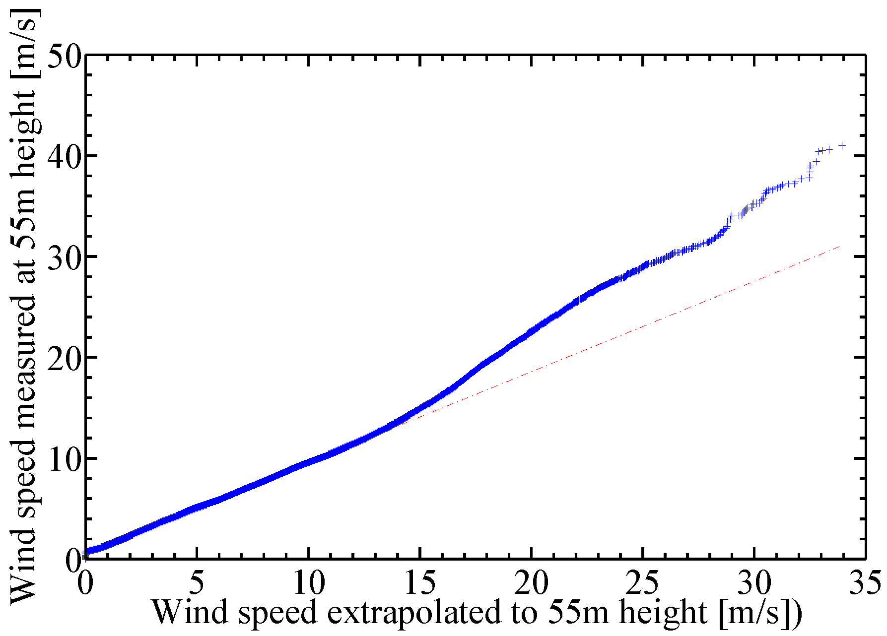
  • Confirm the power law equation by comparing transformed wind speed observations at 10 m to wind speed observations at 55 m
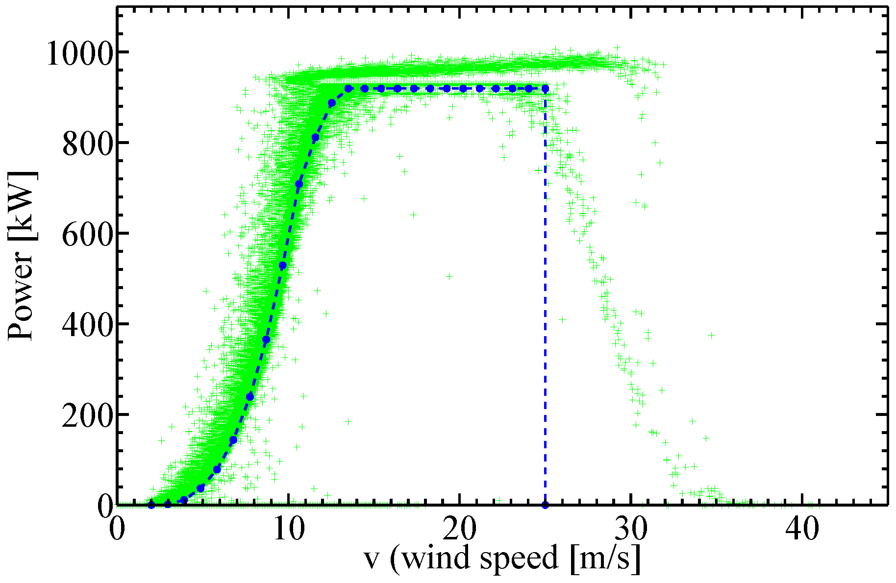
  • Verify the power curve of the test wind turbines (Enercon E44 900 kW) by comparing the calculation to the actual power production data
• Verification of method

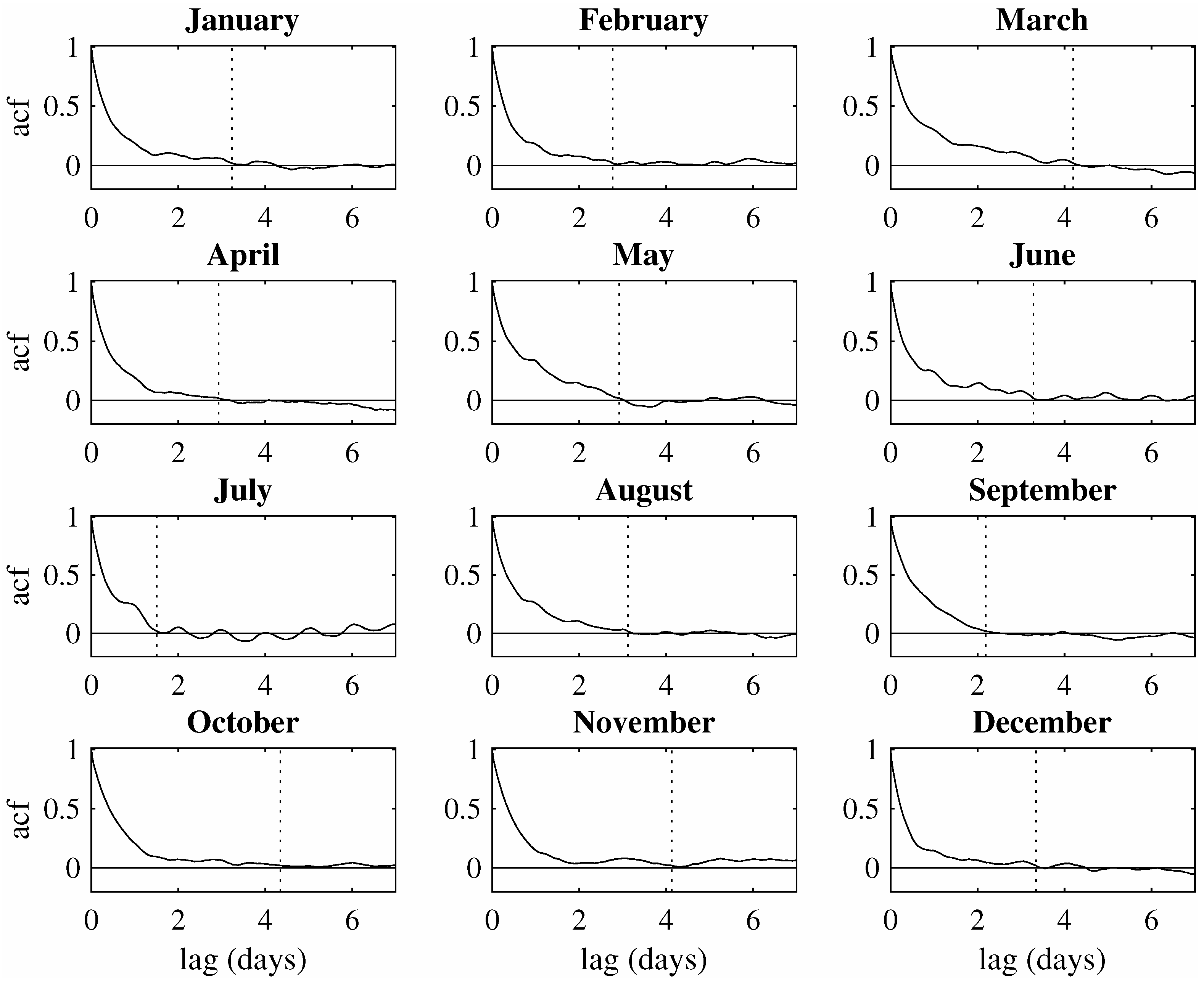
  • Conduct autocorrelation analysis of the wind speed data to determine the length of blocks in the MC wind speed simulation
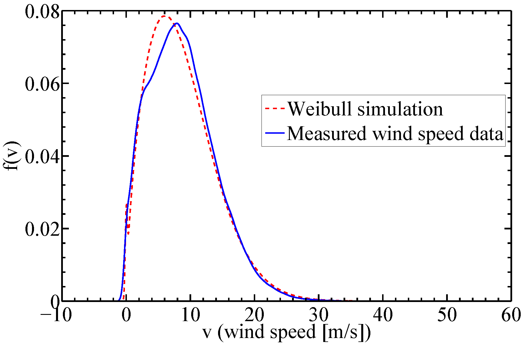
  • Generate estimates of the wind speed densities based on the MC wind speed simulation and the Weibull wind speed simulation and compare these estimates to the density based on actual wind speed observations from the site; This is done at a 55 m measurement height
  • Simulate AEP assuming the test wind turbines based on the Enercon E44 900 kW power curve and compare these values to the observed AEP to evaluate the accuracy of the two wind speed simulations

The following sections describe the relevant tools used in this article.

2.2. Power Law

The IEC Standard uses the power law when measurements at one height (usually called the reference height) are available, but not at wind turbine hub height. In this case, the are some measurements but they are limited to a few years. The power law is considered as a good approximation in these situations and is given by [16],

$$U\left(z\right)=U_{\mathrm{ref}}{\left(\frac{z}{z_{\mathrm{ref}}}\right)}^{\mathsf{\alpha }}$$

(1)

where $U_{\mathrm{ref}}$ is the measurement available at the reference height, z is the turbine hub height, $z_{\mathrm{ref}}$ is the reference height and $\mathsf{\alpha }$ is the wind shear exponent (normally between 0.1 and 0.2). According to the IEC standard, the wind shear exponent can not exceed 0.2 and has to be positive. The standard sets these requirements to avoid enhanced fatigue damage and the risk of blade-tower interaction, which can occur with negative shear [16].

2.3. Weibull Wind Speed Simulation

Weibull wind speed simulation is an established method for wind speed simulation in the wind energy industry. Thus, it is used to for comparison to the wind MC simulation method. The pdf function of the Weibull distribution is given by:

$$p\left(y\right)=\frac{\mathsf{\gamma }}{{\mathsf{\beta }}^{\mathsf{\gamma }}}{y}^{\mathsf{\gamma }-1}exp\left(-{\left(\frac{y}{\mathsf{\beta }}\right)}^{\mathsf{\gamma }}\right),y\ge 0,$$

(2)

where $\mathsf{\gamma }$ is the shape parameter and $\mathsf{\beta }$ is the scale parameter, $\mathsf{\gamma }>0$, $\mathsf{\beta }>0$; see [17]. Here, the variable y will denote wind speed (m/s) in the Weibull simulation. The mean and the variance of the Weibull density function are given by:

$$\mathsf{\mu }=\mathsf{\beta }\Gamma (1+{\mathsf{\gamma }}^{-1}),$$

(3)

$${\mathsf{\sigma }}^2={\mathsf{\beta }}^2\{\Gamma (1+2{\mathsf{\gamma }}^{-1})-{\Gamma }^2(1+{\mathsf{\gamma }}^{-1}\left)\right\}$$

(4)

where $\Gamma (·)$ is the gamma function. Various methods have been used to determine the shape and scale parameters of the Weibull distribution function. Analytical and empirical methods used to find the Weibull parameters are often referred to as classical methods. Other methods match the average wind power density and the occurrences above average wind speed to the Weibull distribution [18]. Discrepancies can appear between measured and statistical distributions. However, because of measurement errors or lack of data, the statistical distribution may be considered as more representative for the long term compared to a sample of measured data [18]. In this research, the built-in MATLAB function wblfit was used to compute maximum likelihood estimates of the Weibull shape and scale parameters. Here, a slight modification to a Weibull simulation, based on a single density, was made. It is unreasonable to fit one Weibull distribution to all data from a single site, due to the fact that wind distribution is different between yearly seasons [19]. The modification lies in dividing the wind speed data into wind directional sectors, as wind direction tends to depend on yearly seasons. A Weibull distribution was fitted to data within each of the eight selected wind speed sectors, which are divided by the north-south line, the northeast-southwest line, the east-west line and the northwest-southeast line. Dividing the data into directional sectors should give a better Weibull distribution fit, since dominant wind direction tends to change according to seasons, and the wind speed varies with season. This method of dividing the wind data into directional sectors was presented by Torres et al. [20]. It characterizes wind speed data according to wind direction. The simulation of wind speed samples based on the eight fitted Weibull distributions is conducted by randomly selecting the sector according to the estimated probability of being within each sector, then a wind speed value is simulated from the fitted Weibull distribution of the selected sector.

2.4. Annual Energy Production

The simulation data can be used to estimate the AEP of a specific turbine. The AEP equation is given by:

$$E=T·f{\int }_0^{\infty }p\left(U\right)P\left(U\right)dU$$

(5)

where T is the time length of one year, f is the frequency, $p\left(U\right)$ is the pdf of the wind speed and $P\left(U\right)$ is the power curve of the selected turbine for the site [16].

2.5. Data

Wind speed data were gathered from two sources: the Icelandic Meteorological Office and Landsvirkjun, the national power company of Iceland. The data from the Icelandic Meteorological Office were wind speed observations at a 10 m height in the period from February 2004 to January 2014. The data from Landsvirkjun contained one year of wind speed observations (10 min average values) at a 55 m height from February 2013 to January 2014. The power law was used to extrapolate the data from a 10 m height to 55 m at the desired wind power production. Unusual and unrealistic wind speed observations were filtered from the raw wind speed data.

Data on observed power production output from two 900 kW test turbines at Burfell were provided by Landsvirkjun. The data are given in AEP in MWh and are from the period February 2013 to January 2014.

3. Development of a Monte Carlo Method

This section introduces the Monte Carlo wind speed simulation and how it works.

3.1. Monte Carlo Wind Speed Simulation

The generation of wind speed samples with the proposed Monte Carlo wind speed simulation is described here. This simulation relies solely on historical wind speed data at the site, accommodated with simple sampling techniques and autocorrelation information on wind speed data. The motivation for developing the MC wind speed simulation is to establish a robust and generic simulation of wind speed samples that is such that the seasonality and the autocorrelation structure of the true wind speed are reserved. Further, these wind speed samples are used with the relevant wind turbine power curve to obtain the distribution of the potential AEP at the site. As the seasonality and the autocorrelation of the wind speed is reserved, the variance of the simulated potential AEP is closer to the variance of the observed potential AEP than the variance of the potential AEP that is simulated assuming independence in wind speed.

The MC wind speed simulation is setup as follows. Samples of wind speed are generated at the specific site by resampling historical data. No distributional assumptions are made. The recommended minimum amount of historical data for the simulation is 10 years of data. It is assumed that there is no trend in the historical data and that the distribution describing the vector of wind speed at discrete time points over a whole year is the same across the years over which the historical data were observed. Further, this same distribution is assumed for the wind speed vector of the year over which predictions are desired.

Based on the calculations of the sample autocorrelation of the wind speed data within each of the months at the given site, the minimum lag needed for the autocorrelation to fade out is determined. This minimum lag is measured in days and denoted by d. The quantity d is then used to determine the length of consecutive blocks. These d day blocks will be used as sampling units in the MC wind speed simulation as opposed to sampling each value independently. With the d day blocks as the sampling units, the autocorrelation in the wind speed process is reserved while using 10-min values or hourly values as sampling units, and sampling these values independently does not reserve the autocorrelation.

All observed data on wind speed are divided into consecutive d day blocks. To simulate a single sample over one year, each of the $(365/d)$ blocks within a year are sampled from the corresponding blocks in the previous N years, where $\left(x\right)$ gives the largest integer less than x, and the last block of the year will be longer than or equal to d days and less than $2d$ days. The first d day block of the sample is drawn with equal probability ($1/N$) from the first d day block of the previous N years. Likewise, the second d day block of the sample (the $(d+1)$-th day to the $2d$-th day of the year) is drawn independently of the first block with equal probability ($1/N$) from the second d day block of the previous N years, and so on, for the other d day blocks of the year. By repeating this process L times, L samples of yearly wind speed samples are obtained.

It is important that the simulation reserves the seasonality and the autocorrelation in the data without making assumptions about underlying seasonality and autocorrelation, as wind speed is higher in the winter compared to the summer [18], and the autocorrelation is present and changing over the year. Thus, the parameter d must be selected such that the autocorrelation is reserved. One way to ensure this is to select d such that the autocorrelation at lag d is negligible. The sample autocorrelation is computed from the raw data after they have been standardized with respect to seasonal mean, seasonal standard deviation and daily variability. The most straight forward correction is based on fitting a constant, sine and cosine functions with appropriate frequencies to the mean and the standard deviation. It is suggested that the sample autocorrelation is calculated within each month using only data from that month, as the autocorrelation is different between months. Then, these sample autocorrelations are used to determine at what lag the autocorrelation becomes none influential. Here, it is assumed that the smallest lag at which the sample autocorrelation goes below $0.02$ is the smallest lag at which the autocorrelation is labeled as none influential within the given month (also labeled as none influential for larger lags). Then, d is set equal to the largest none influential lag across the months.

3.2. The Method as a Procedure

The method introduced in the previous subsection is formulated here as a procedure for the ease of use. There are two aspect to the approach, the quality of the data and the actual simulation. The quality aspect should be considered before using this method. The following should be taken into account:

• In order to represent wind speed reasonably well, get a minimum of N = 10 years of actual/observed wind data for the relevant site. Note that the method does not assume any distribution. It is assumed that there is no trend in the data.
• If data are not available at the correct height, use the power law to extrapolate and verify the result if possible.
• For AEP calculations, make sure that the power curve for the selected wind turbine is correct.

Having the prerequisites in order, the steps of the MC wind speed simulation are as follows:

• Estimate the seasonal mean, the seasonal standard deviation and the daily variability of the raw data.
• Compute standardized residuals by subtracting the estimated seasonal mean and the daily variability from the raw data and scaling the difference with respect to the estimated seasonal standard deviation.
• Group the standardized residuals into a fixed time interval (e.g., months).
• Calculate the sample autocorrelations for each interval using the standardized residuals.
• Plot the sample autocorrelation for individual months for visual inspection. The smallest lag, such that the sample autocorrelation goes below 0.02, is defined as the lag where the autocorrelation becomes none influential.
• Select the block size (parameter d), such that the sample autocorrelation is none influential in all months for lag d, but still as low as possible.
• Regroup all of the data into d day blocks, so that they fit into one year $(365/d)$, i.e., a sequence of blocks forms one year. Each block location is numbered and positioned in the same place in the year sequence. The last block of the year will be longer than or equal to d days and less than $2d$ days.
• A simulation of the wind speed set is made as follows:

  • Each of the $(365/d)$ blocks within a year are sampled from the corresponding blocks in the previous N years, that is the first d day block of the sample is drawn with equal probability ($1/N$) from the first d day block of the previous N years.
  • Likewise, the second d day block of the sample (the $(d+1)$-th day to the $2d$-th day of the year) is drawn independently of the first block with equal probability ($1/N$) from the second d day block of the previous N years, and so on, for the other d day blocks of the year.
  • The previous two steps are repeated L times to obtain L samples of yearly wind speed. L should be at least 1000.
• For each of the L years, an AEP is calculated.
• The mean and 95% interval for AEP is then calculated from the L simulated AEP values.

In Section 5, the MC wind speed simulation is applied to data from Burfell in Iceland; it is demonstrated how d is selected, and the frequency of the sine and cosine functions are given.

4. Verification of Data

To test the suggested MC wind speed simulation, a test site was used. It is the Burfell site in southeast Iceland. The site is described in detail in the authors previous work [5]. The process is first to verify the data and then the method. First, the data were filtered with respect to unusual and unrealistic wind speed observations. Then, the data were verified in terms of both the extrapolation from 10 m to 55 m and the power curve of the wind turbines.

4.1. Extrapolated Data Compared to Measured Data

Due to the fact that limited wind speed data from the desired height of 55 m was available, the power law was used to extrapolate the historical data measured. Before the data were extrapolated, the accuracy of the power law extrapolation was evaluated. The calculated wind shear factor $\mathsf{\alpha }$ = 0.1309 and its 95% bootstrap confidence interval (0.1192 to 0.1399) was used to extrapolate wind data from Burfell measured at a 10 m height to a 55 m height, and then, it was compared to measured data at a 55 m height. The data used for the comparison were measured between February 2013 and January 2014. A quantile-quantile plot was made to determine whether the wind speed extrapolated to a 55 m height came from the same distribution as measured wind speed at a 55 m height. The plot is shown in Figure 1; it was generated using the built in MATLAB function qqplot. A red reference line is drawn on the plot to help judge linearity. Linearity means that the extrapolated data come from the same distribution as the data measured at the 55 m height. One can see that the points appear to be approximately linear up to a wind speed of around 15 m/s. At a wind speed above 15 m/s, the power law appears to underestimate the wind speed.

Based on these calculations, it has been shown that the wind shear factor $\mathsf{\alpha }$ of 0.1309 can be used to extrapolate the wind speed data measured at a 10 m height up to the desired wind turbine height. This verifies that the power law is applicable at Burfell; the deviation in the power law approximation has however been noted at wind speeds above 15 m/s. Note that the mean wind speed at Burfell is 8.73 m/s, which means that the power law can extrapolate most of the wind with high accuracy.

This verification step using the power law was needed in this study, as it is recommended that the MC wind speed simulation is based on at least 10 years of historical wind speed data at the site of interest. Since these data were only available measured at a 10 m height, the power law was used to extrapolate the wind speed to the desired height. Note that if the available historical data are measured at the desired height, then the use of the power law is not needed in the MC wind speed simulation.

4.2. Power Curve Compared to Actual Power Production

Figure 2 shows that the power curve gives a conservative estimate of the potential AEP at Burfell; the estimated power curve for the Enercon E44 turbine presented by Enercon [21] is plotted on top of measured power curve. Notice that the estimated power curve lies within the lower scatter points of the measured curve, which shows that the Enercon power curve is a conservative estimate, i.e., at approximately mean wind speed at Burfell or 9 m/s, the measured power is 32.7% higher on average. It is noticeable in Figure 2 that the E44 wind turbine is producing power after the referenced “cut-out” wind speed set at 25 m/s by the Enercon power curve. This power production is explained with the “storm control” feature installed in the Enercon wind turbines. The storm control feature enables wind turbines from Enercon to produce power.

This extensive “over” production experienced from the two E44 wind turbines is explained essentially by two factors; firstly, because Enercon is seemingly on purpose underestimating the potential power production of their wind turbines in their published power curves; Enercon publishes a power curve, which reflects the power production Enercon can guarantee from their wind turbines; secondly, because of surprisingly good performance in Icelandic conditions from the storm control feature installed in the Enercon wind turbines. The storm control feature enables the Enercon turbines to keep producing energy at wind speeds from 25 m/s to 34 m/s. Even though the referenced cut-out wind speed for their wind turbine estimated power curves is set at 25 m/s, Icelandic conditions perhaps include more wind speed values from 25 m/s to 34 m/s than normally experienced by Enercon, because Enercon states that their estimated power curves include effects from Enercon storm control technology.

5. Verification of Method

Here, the two wind simulation approaches presented in Section 2 are used to generate samples that represent the wind speed distribution at Burfell. The validity of the two simulation approaches will be verified by comparing their wind speed samples to the observed wind speed and also by comparing their corresponding AEP to the observed AEP. Landsvirkjun has installed two Enercon E44 900-kW wind turbines at the Burfell site, so the observed AEP is from these turbines, and the simulated AEP corresponding to the two wind speed simulations is calculated by transforming wind speed values to energy production via the power curve of the Enercon E44 900-kW wind turbine.

5.1. Determination of d in the MC Wind Speed Simulation

Here, it is demonstrated how the parameter d in the MC wind speed simulation for the Burfell data is selected. It was concluded, based on the sample autocorrelation, that autocorrelation in wind speed at Burfell becomes non-influential at lags of length from one and a half day to almost five days as can be seen in Figure 3. The weakest autocorrelation found in the data occurs in July, where autocorrelation becomes none influential after approximately one and a half days. The longest sustained autocorrelation in the wind speed data occurs in March, October and November, where autocorrelation becomes none influential between four and five days. In general, the sample autocorrelation becomes none influential after five days for all months. Therefore, for this particular site, a five-day block division was selected, that is $d=5$ was selected.

Note that the autocorrelation was calculated using standardized residuals. The estimated mean was found using regression based on a constant, sine and cosine function with periods (measured in days) of lengths $1.00$, $73.05$, $91.31$, $121.75$, $182.63$ and $365.25$. The estimated standard deviation was found using the same regression model for the absolute value of the observed wind speed minus the estimated mean.

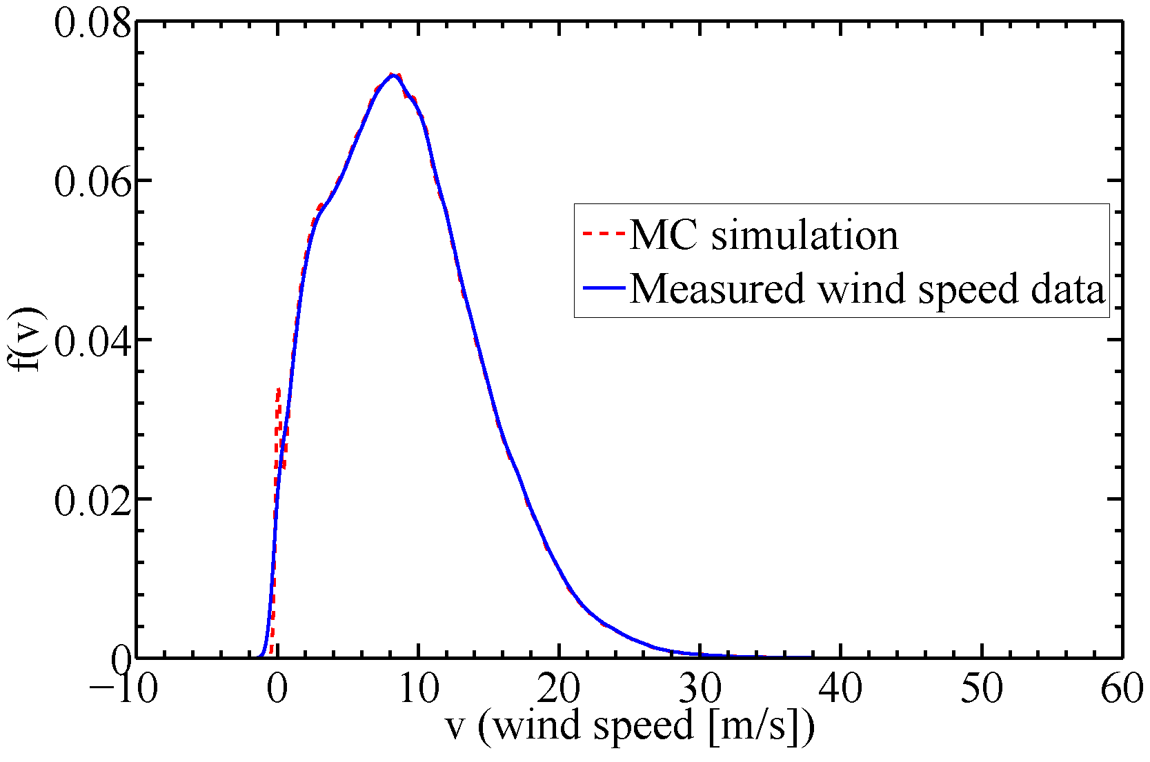
5.2. Wind Speed Simulation at Burfell Using the Monte Carlo Approach and the Weibull Approach

In this section, the results from the two wind speed simulation approaches are presented, including a comparison and evaluation of the two approaches. The observed wind speed at Burfell and wind speed samples of the Weibull wind speed simulation are presented in Figure 4 and

Table 1. Summary statistics for the observed wind speed at Burfell at a 55 m height, the samples of the Weibull wind speed simulation and the samples of the MC wind speed simulation.

Wind Speed at Burfell	Mean (m/s)	Median (m/s)	Std (m/s)
Observed	8.73	8.24	5.18
Weibull simulation	8.70	7.93	5.29
MC simulation	8.71	8.20	5.19

. The marginal pdfs of the samples of the Weibull wind speed simulation and of the observed data are close; there is, however, a slight deviation at the top of the pdfs. The sample means of the Weibull wind speed simulation samples and the observed data at Burfell are close, and the same is true for the sample standard deviations; see Table 1.

The results of MC wind speed simulation and its comparison to the observed data at Burfell are presented in Figure 5 and Table 1. From Figure 5, it can be seen that the marginal pdf of the simulated samples gives a good match to the pdf of the observed data, which is not surprising, as the simulated samples are solely based on the observed data. The summary statistics from Table 1 verify that the MC wind speed simulation gives a good match to the observed data.

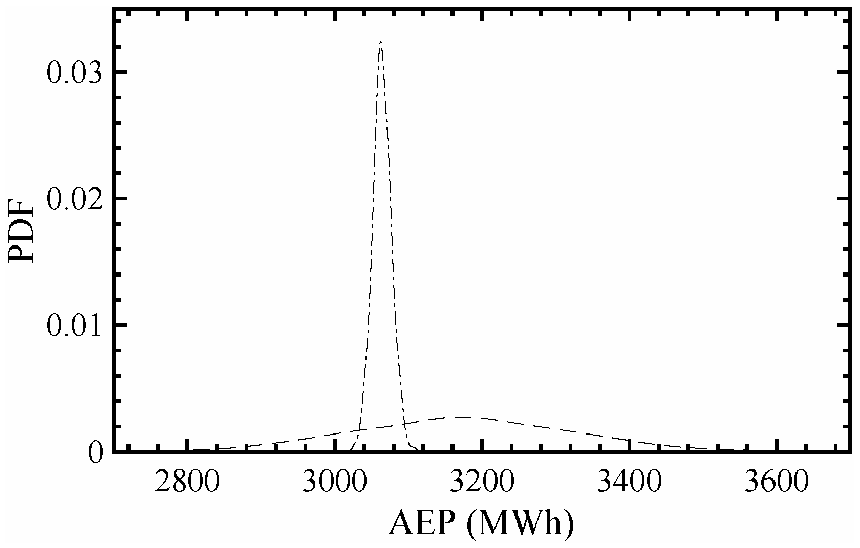
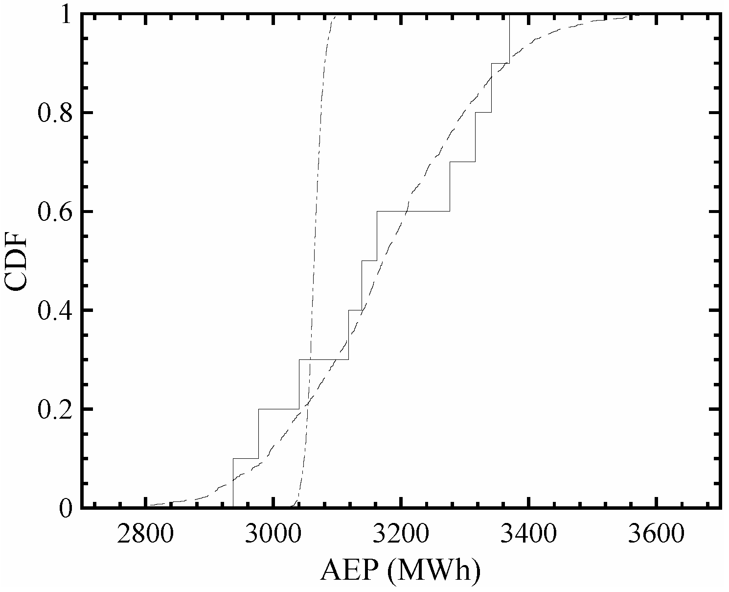
5.3. Comparison of Simulated AEP and Observed AEP

Measured power production output data from the two E44 900 kW test turbines at Burfell (Turbines 1 and 2) from the period February 2013 to January 2014 are presented in terms of AEP in MWh in

Table 2. Observed annual energy production (AEP) and scaled AEP for two E44 900 kW wind turbines at Burfell for one year (1 February 2013 to 31 January 2014).

Burfell	Turbine 1	Turbine 2
Observed AEP (MWh)	3185	2939
Scaled AEP (MWh)	3228	3297

.

It is noticeable from Table 2 that the AEP for each wind turbine is slightly different. This difference is caused by different availability between the two turbines. Each turbine experienced different amounts of downtime caused by malfunction. The measured data from Table 2 have to be scaled according to the availability data for the two E44 900 kW turbines. The scaling makes sure that measured and calculated results are being compared with the same amount of production hours in the year. The scaled data for the measured AEP are presented in Table 2. The reason for this is that simulated AEP assumes constant power production throughout the year, a 24/7 production.

The two E44 900 kW turbines are placed side by side, and thus, they should produce almost the same amount of energy. To make the AEP values similar for comparison a scaling of the measured AEP was done by using the availability data for each turbine. The values in the last row of Table 2 can consequently be used to compare observed AEP and simulated AEP.

The AEP for a E44 900 kW turbine (the same type as Turbines 1 and 2) was simulated 1000 times based on 1000 simulated wind speed time series each spanning a year-long period, using both the MC wind speed simulation and the Weibull wind speed simulation. Each sample of simulated wind speed time series is transformed to AEP through the wind power curve shown in Figure 2.

For each wind speed sample spanning a year based on the MC or the Weibull wind speed simulations, the AEP is calculated using Equation (5). The median AEP (P50), the 10-th percentile of AEP (P90) and the 95% prediction interval for AEP are presented in

Table 3. AEP based on MC wind speed simulation and Weibull wind speed simulation in the case of the E44 900-kW wind turbine (55 m hub height).

Burfell	P50	P90	95% Prediction Interval
MC AEP (MWh)	3172	2985	(2926; 3403)
Weibull AEP (MWh)	3064	3048	(3042; 3084)

and Figure 6. Notice that the prediction interval for AEP based on the Weibull wind speed simulation is quite narrow compared to the one based on the MC wind speed simulation. This is also evident in Figure 6, which shows the probability density of the simulated AEP based on the two approaches. The MC wind speed simulation takes into account autocorrelation in wind, by simulating blocks of wind speed. On the other hand, the Weibull wind speed simulation generates independent values, meaning that one simulated 10-min average wind speed is not correlated to the next one. This type of simulation gives a reasonable estimate of the median wind speed; however, it does not manage to replicate the variation in wind speed between years due to the absence of temporal dependence in the wind speed simulation, hence the narrow 95% prediction interval for the AEP.

The result for AEP calculated with the Weibull method is slightly higher than the 2870 MWh, another group obtained also using Weibull on the Burfell site [22]. P50 based on MC wind speed simulation is greater than P50 based on the Weibull wind speed simulation. However, P90 is smaller in the case of the MC wind speed simulation compared to P90 of the Weibull wind speed simulation. The results show that the 95% prediction interval for AEP calculated based on the MC wind speed simulation is eleven-times wider than the 95% prediction interval based on the Weibull wind speed simulation. Notice that the Weibull AEP calculations of Perkin et al. [22] are close to falling within the prediction interval of the MC wind speed simulation. These results show that by taking the autocorrelation in wind speed into account, the variation in wind speed can be replicated better, compared to a simulation approach that assumes independence, like the Weibull wind speed simulation, hence the wider 95% prediction interval in Table 3.

By using 10 years of wind speed data (2004 to 2013) from Burfell and transforming them to AEP data using the power curve of the E44 900 kW wind turbine, estimates of the AEP corresponding to the actual observed wind speed at Burfell for the years 2004 to 2013 are obtained. These ten estimates of actual AEP are compared to the simulated AEP based on the MC wind speed simulation and the Weibull wind speed simulation. Note that these two simulation methods use the same power curve and the same wind speed data. The cdf of the ten estimates of actual AEP is shown in Figure 7 along with the cdfs of AEP based on the two simulation methods. It is clear that the distribution of AEP based the MC wind speed simulation is much closer to the estimated AEP for the last ten years than the distribution of AEP based the Weibull wind speed simulation. What can be learned from Figure 7 is that P90 is overestimated, and P50 and the scale of the AEP are underestimated using the Weibull wind speed simulation, while the MC wind speed simulation is in close agreement with P90, P50 and the scale of the AEP.

6. Conclusions

The biggest edge that the MC wind speed simulation has over the Weibull wind speed simulation is the fact that when calculating the AEP for a given site, the simulated values of AEP give a representative distribution of the power production of the site. Another advantage of the MC wind speed simulation is its simplicity relative to the simulation methods for wind speed that aim at including the autocorrelation and seasonal effects for AEP computation. This simplicity stems from not making distributional assumptions and a simple resampling scheme. A forecast of the future 25 years (typical lifetime of a wind park) of wind speed and AEP can be drawn from the distribution of simulated wind speed values corresponding to a given site. This type of forecasting could be performed using solely 10 years of historical data. Unlike the MC wind speed simulation, the Weibull simulation method does not take into account autocorrelation and seasonal effects in wind speed distribution. The effect of this difference is that simulation of AEP based on the MC wind speed simulation is in close agreement with P90, P50 and the scale of the actual AEP, while the Weibull wind speed simulation overestimates P90 and underestimates both P50 and the scale of AEP. The MC wind speed simulation is a novel approach for estimating wind speed distribution, and the corresponding AEP and is a contribution to wind energy research.

References

1. Chehouri, A.; Younes, R.; Ilinca, A.; Perron, J. Review of performance optimization techniques applied to wind turbines. Appl. Energy 2015, 142, 361–388. [Google Scholar] [CrossRef]
2. Carta, J.A.; Ramirez, P.; Velazquez, S. A review of wind speed probability distributions used in wind energy analysis case studies in the canary islands. Renew. Sustain. Energy Rev. 2009, 13, 933–955. [Google Scholar] [CrossRef]
3. Rocha, P.A.C.; De Sousa, R.C.; De Andrade, C.F.; Da Silva, M.E.V. Comparison of seven numerical methods for determining Weibull parameters for wind energy generation in the northeast region of brazil. Appl. Energy 2012, 89, 395–400. [Google Scholar] [CrossRef]
4. Chang, T.P. Performance comparison of six numerical methods in estimating Weibull parameters for wind energy application. Appl. Energy 2011, 88, 272–282. [Google Scholar] [CrossRef]
5. Ragnarsson, B.; Oddsson, G.V.; Unnthorsson, R.; Hrafnkelsson, B. Levelized cost of energy analysis of a wind power generation system at burfell in iceland. Energies 2015, 8, 9464–9485. [Google Scholar] [CrossRef]
6. Usta, I.; Kantar, Y.M. Analysis of some flexible families of distributions for estimation of wind speed distributions. Appl. Energy 2012, 89, 355–367. [Google Scholar] [CrossRef]
7. Zhou, J.; Erdem, E.; Li, G.; Shi, J. Comprehensive evaluation of wind speed distribution models: A case study for north dakota sites. Energy Convers. Manag. 2010, 51, 1449–1458. [Google Scholar] [CrossRef]
8. Carta, J.A.; Velázquez, S.; Cabrera, P. A review of measure-correlate-predict (mcp) methods used to estimate long-term wind characteristics at a target site. Renew. Sustain. Energy Rev. 2013, 27, 362–400. [Google Scholar] [CrossRef]
9. Jung, S.; Kwon, S.-D. Weighted error functions in artificial neural networks for improved wind energy potential estimation. Appl. Energy 2013, 111, 778–790. [Google Scholar] [CrossRef]
10. Jung, S.; Vanli, O.A.; Kwon, S.-D. Wind energy potential assessment considering the uncertainties due to limited data. Appl. Energy 2013, 102, 1492–1503. [Google Scholar] [CrossRef]
11. Kwon, S.-D. Uncertainty analysis of wind energy potential assessment. Appl. Energy 2010, 87, 856–865. [Google Scholar] [CrossRef]
12. Pedersen, T.F.; Gjerding, S.; Ingham, P.; Enevoldsen, P.; Jesper, H.K. Wind Turbine Power Performance Verification in Complex Terrain and Wind Farms; Report; RISO National Laboratory: Roskilde, Denmark, 2002.
13. Lackner, M.A.; Rogers, A.L.; Manwell, J.F. Uncertainty analysis in mcp-based wind resource assessment and energy production estimation. J. Solar Energy Eng. Trans. ASME 2008, 130. [Google Scholar] [CrossRef]
14. Bensoussan, A.; Bertrand, P.R.; Brouste, A. Forecasting the Energy Produced by a Windmill on a Yearly Basis. Stoch. Environ. Res. Risk Assess. 2012, 26, 1109–1122. [Google Scholar] [CrossRef]
15. Gass, V.; Strauss, F.; Schmidt, J.; Schmid, E. Assessing the effect of wind power uncertainty on profitability. Renew. Sustain. Energy Rev. 2011, 15, 2677–2683. [Google Scholar] [CrossRef]
16. Berg, J.; Mann, J.; Nielsen, M. Introduction to Micro Meteorology for Wind Energy; Denmarks Tekniske Universitet (DTU): Kgs Lyngby, Denmark, 2013. [Google Scholar]
17. Meeker, W.Q.; Escobar, L.A. Statistical Methods for Reliability Data; Wiley: New York, NY, USA, 1998. [Google Scholar]
18. Nawri, N.; Petersen, G.N.; Bjornsson, H.; Hahmann, A.N.; Jonasson, K.; Hasager, C.B.; Clausen, N.E. The wind energy potential of Iceland. Renew. Energy 2014, 69, 290–299. [Google Scholar] [CrossRef]
19. Petersen, J.B.; Birgisson, T.; Bjornsson, H.; Jonasson, K.; Petersen, G.N. Vindhradamaelingar og Sambreytni Vinds; Icelandic Meteorological Office: Reykjavik, Iceland, 2011. [Google Scholar]
20. Torres, J.L.; Garcia, A.; Prieto, E.; Francisco, A.D. Characterization of wind speed data according to wind direction. Solar Energy 1999, 66, 57–64. [Google Scholar] [CrossRef]
21. Enercon. Enercon Product Overview; Enercon Wind Turbine Manufacturer: Bremen, Germany, 2012. [Google Scholar]
22. Perkin, S.; Garrett, D.; Jensson, P. Optimal wind turbine selection methodology: A case-study for burfell, iceland. Renew. Energy 2015, 75, 165–172. [Google Scholar] [CrossRef]
Figure 1. Quantile-Quantile Plot (QQ-plot) of measured data at 55 m vs. data measured at 10 m extrapolated to a 55 m height.
Energies 09 00286 g001
Figure 2. Measured power curve vs. estimated curve for the E44 900 kW turbine.
Energies 09 00286 g002
Figure 3. Autocorrelation plots for the twelve months of the year with lag measured in days.
Energies 09 00286 g003
Figure 4. Sample probability density functions (pdfs) based on the observed wind speed at Burfell and samples of the Weibull wind speed simulation.
Energies 09 00286 g004
Figure 5. pdf plot of MC simulated wind at Burfell.
Energies 09 00286 g005
Figure 6. pdfs of MC simulated AEP (dashed curve) and Weibull simulated AEP (dash-dot curve) for a E44 900 kW wind turbine (same type as Turbines 1 and 2 at Burfell).
Energies 09 00286 g006
Figure 7. cdfs of MC-simulated AEP (dashed curve) and Weibull-simulated AEP (dash-dot curve) for a E44 900 kW wind turbine and the observed AEP (solid curve) at Burfell for the same type of turbine (Turbine 1).
Energies 09 00286 g007