1. Introduction
Nowadays, wind power is considered as one of the most viable and sustainable resources worldwide [
1]. Wind turbines often operate offshore in order to take advantage of stronger and more reliable winds; however, unscheduled maintenance due to unexpected failures can be costly, not only for maintenance support but also due to lost production time [
2]. Condition monitoring systems (CMS) can play a pivotal role in establishing a condition-based maintenance and asset management. Most modern wind turbines incorporate on-board supervisory control and data acquisition (SCADA) systems for control and monitoring of turbine operation and performance. A SCADA system may contain massive amounts of data related to hundreds of parameters of the wind turbines, which has attracted great research interests in fault diagnosis and prognosis for wind turbines.
Usually, one or more parameters generated by SCADA systems are selected and used to obtain models of the turbines operating under different conditions. There are two types of modelling methods: mechanistic methods and data driven model-based methods. The former require a thorough understanding of the process and may result in complex models. The latter do not require knowledge of the process or specific parameters; they are obtained directly from measured input and output signals [
3]. For example, Marvuglia [
4] investigated an artificial neural network (ANN) model of the relationship between wind speed and generated power for an entire wind farm. The power curves modelled in this way are used to detect faults of the wind farm as a whole. Philip
et al. [
5] proposed a multiple-input (wind speed and active power) single-output (gearbox bearing temperature) state dependent parameter (SDP) method; multivariate SDP models were used to identify the distinct warning levels of a developing fault using adaptive thresholds.
At the same time, in order for the SCADA system to work more accurately, it is essential to obtain enough information about the wind turbine’s operational condition and performance. This can be done by using different types of sensors and by monitoring different locations within the wind turbine. Due to the complexity of the turbine, there could be more than 250 monitoring points required to monitor most subsystems of a turbine; the number of the monitoring points will thus be considerably larger for a wind farm [
6]. Apart from the large amount of data needing to be handled and transmitted, other questions may have also risen; for example, concerning the redundancy among monitoring data, many of the signals might be highly correlated.
This paper therefore proposes a novel model built using parallel factor analysis (PARAFAC) for fault detection and sensor selection of wind turbines based on SCADA data. As with other related decomposition methods, such as Tucker3 [
7] and unfolded principal component analysis (PCA) [
8], PARAFAC belongs to the same family of bi-linear or multi-linear methods of decomposing multi-way data into a set of loading and score matrices. However, PARAFAC uses less degrees of freedom than Tucker3 or unfolded PCA methods. This intrinsic feature leads to simpler models and avoids the incorporation of non-significant effects such as noise and redundant information in the model. Originated from psychometrics [
9], PARAFAC has attracted increasing interest because it is a processing technique capable of simultaneously determining the pure contributions to the dataset and optimising each factor at a time in trilinear systems. Therefore it has been used in psychology, chemometrics and other areas [
10,
11]. One of the most popular applications is modelling fluorescence excitation-emission data, which is a commonly used data type in chemistry, medicine and food science. Several studies have been done to explore the underlying chemical phenomena in fluorescence spectral data obtained from sugar solutions in order to investigate quality issues [
12] and a fish dataset with known fluorophores [
13]. The main characteristic of this new approach is that it can simultaneously explore information regarding sensor contribution and measurement data contribution at different points. Based on such information, by using an appropriate clustering method, measurement samples can be classified and the sensor array can be optimised. However, this method has not previously been applied to condition monitoring of wind turbines.
This paper is organised as follows: wind turbine data used to evaluate the proposed method are presented and pre-processed in
Section 2.
Section 3 proposes the methodology of the PARAFAC model while
Section 4 presents the
K-means clustering method used to classify measurement data into alarm events, normal and faulty segments. In
Section 5 the models are applied to SCADA data obtained from one of the operational wind turbines where the results are cross checked to ensure real faults have been identified. In
Section 6 conclusions are drawn and suggestions made for future work.
2. Wind Turbine Data
The SCADA data used for this research were obtained from an operational wind farm. For each turbine, a complete history of sensor information and turbine status information for a period of 16 months are available. These data, with a cut-in wind speed of 3 m/s and a cut-out wind speed of 25 m/s, consist of 128 parameters for various temperatures and pressures, power outputs, vibrations, wind speed, digital control signals and others, associated with the condition parameters of blades, nacelle, rotor, generator, gearbox, grid, hydraulic fluid, cooling water, and meteorological conditions. The SCADA system acquires data at a sample rate in the order of 2 s. The data are then processed and stored at 10-minute intervals in order to significantly reduce the amount of data that need to be processed while still reflecting the operation of wind turbines under normal and fault conditions. Thus a total of 77241 measurements are obtained for each parameter for the period of 16 months. The SCADA data from one of the operational wind turbines are selected for analysis and validation of the proposed method. Alarm logs that record the time at which the alarm occurs and the message that reveals the malfunction of particular parameters of the turbine are also available, which are used to cross-check potential faults identified from the data against what was actually happening.
2.1. Data Selection
Data selection is first carried out to eliminate those digital and constant signals, which are ineffective to the PARAFAC analysis. The meteorological parameters such as wind direction, humidity, air pressure, and those parameters representing set points and digital signals from controllers, together with those parameters that remain constant, are removed from the SCADA data. As one of the most important influencing meteorological parameters, the wind speed is still retained, but it is not used for PARAFAC. Thus there are 52 sensor signals left for PARAFAC analysis, which are associated with the parameters defining the performance of the turbine operations, such as the nacelle position (sensor 1); blades positions (sensors 2–8); mains currents (sensors 9–11); apparent power and active power (sensors 12–13); reactive power (sensor 14); pitch motor currents (sensors 15–17); oil pressures (sensors 18–19); oscillation signals (sensors 20–25), speeds of the generator and the rotor (sensors 26–32), temperatures of the generator windings, the gearbox bearings, the nacelle, the gearbox oil sump, the hydraulic fluid and the cooling water (sensors 33–52).
2.2. Data Pre-processing
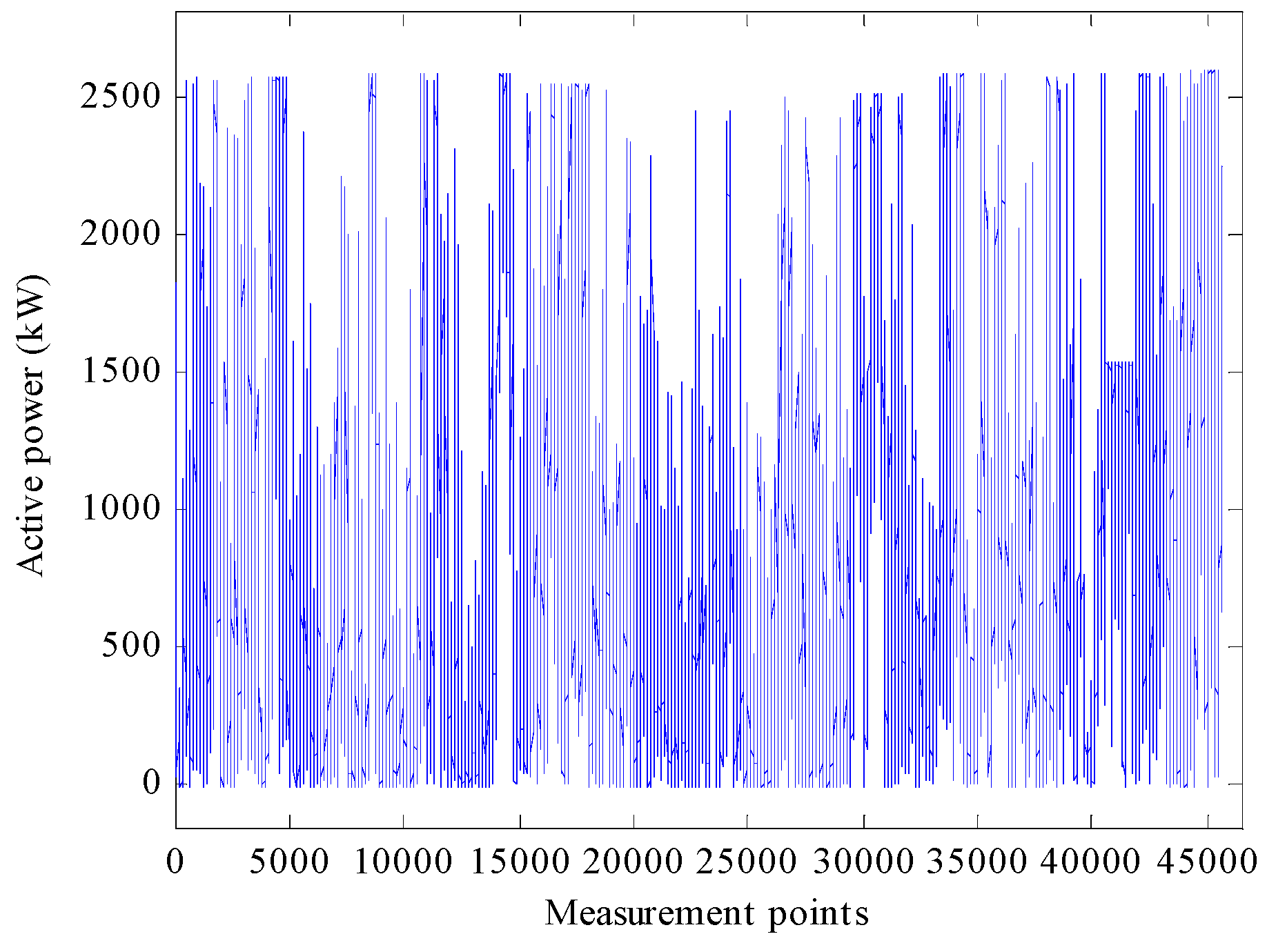
Gaps in SCADA data exist due to occasions when the turbine is inactive during periods of low and high wind speeds. Additional gaps occur due to the occurrence of scheduled maintenance and faults. Prior to the PARAFAC model analysis, it is necessary to remove these gaps. Thus, 45,654 measurement points remained for each turbine parameter. After removal of all the gaps in the data, the active power of the turbine is plotted in
Figure 1 as an example.
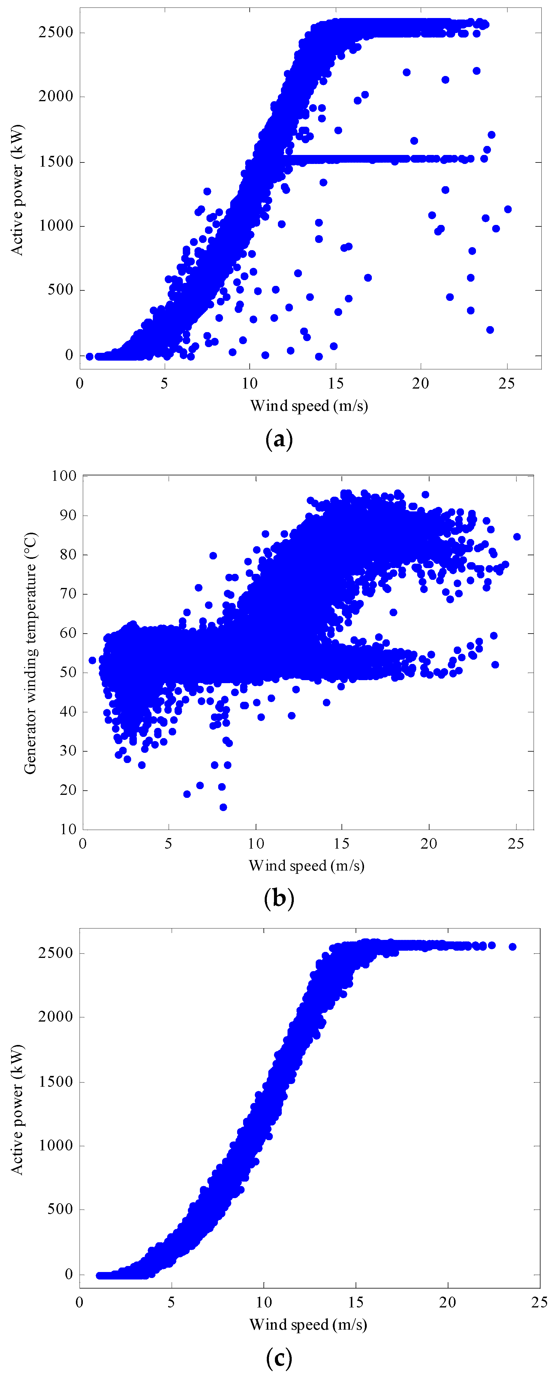
Figure 2a,b show the relationship between wind speed and active power output, and between wind speed and generator winding temperature, respectively.
Figure 2c illustrates the active power output as a function of wind speed of a fault-free turbine for a further reference. As
Figure 2a demonstrates, many measured values of power output fall well inside the range of the normal power curve; so these measurements are defined as normal. However, when the wind speed is higher than 13 m/s, the turbine was operating for some periods of time with a power output reduced to around 1.5 MW and a generator winding temperature reduced to around 58 °C. These measurements indicate the wind turbine is operating in a fault condition. There are some discrete points deviating from the curves which are likely associated with different types of alarms. In our study, in order to investigate the periods of reduced power output and reduced generator winding temperature, only those data samples for which wind speed is higher than 13 m/s are considered. This would be beneficial as the general objective of the modelling process is to identify faults by comparing differences between the normal and the abnormal operational signals. Thus, for each of the 52 sensors used in this study, as explained above, there are 5002 measurements remaining for which wind speed is higher than 13 m/s. The input data of the sensor array can be described as:
4. K-means Clustering Method
In order to verify if the extracted features from the PARAFAC model are good for system identification,
K-means clustering method is used. Essentially,
K-means clustering automatically divides a data set into
K groups [
19]. It proceeds by selecting
k initial cluster centres and then iteratively refining them as follows.
Let
x = {
xi},
i = 1,…,
n be the set of
n dimensional observations to be clustered into a set of
K clusters
c = {
ck},
k = 1,…,
K.
K-means algorithm finds a partition such that the squared error between the empirical mean of a cluster and the points in the cluster is minimised [
20]. Let
uk be the mean of cluster
ck. The squared error between
uk and the points in cluster
ck is defined as:
The goal of
K-means is to minimise the sum of the squared error over all
K clusters:
Minimising this objective function is known to be an non-deterministic polynomial (NP)-hard problem (even for
K = 2) [
21]. Thus
K-means, which is a greedy algorithm, can only converge to a local minimum. One way to overcome the local minima is to run the
K-means algorithm, for a given
K, with multiple different initial partitions and choose the partition with the smallest squared error.
K-means is used with the Euclidean metric for computing the distance between points and cluster centres. Therefore,
K-means tends to find spherical or ball-shaped clusters in data.
5. Results and Discussion
5.1. Data Pre-Processing
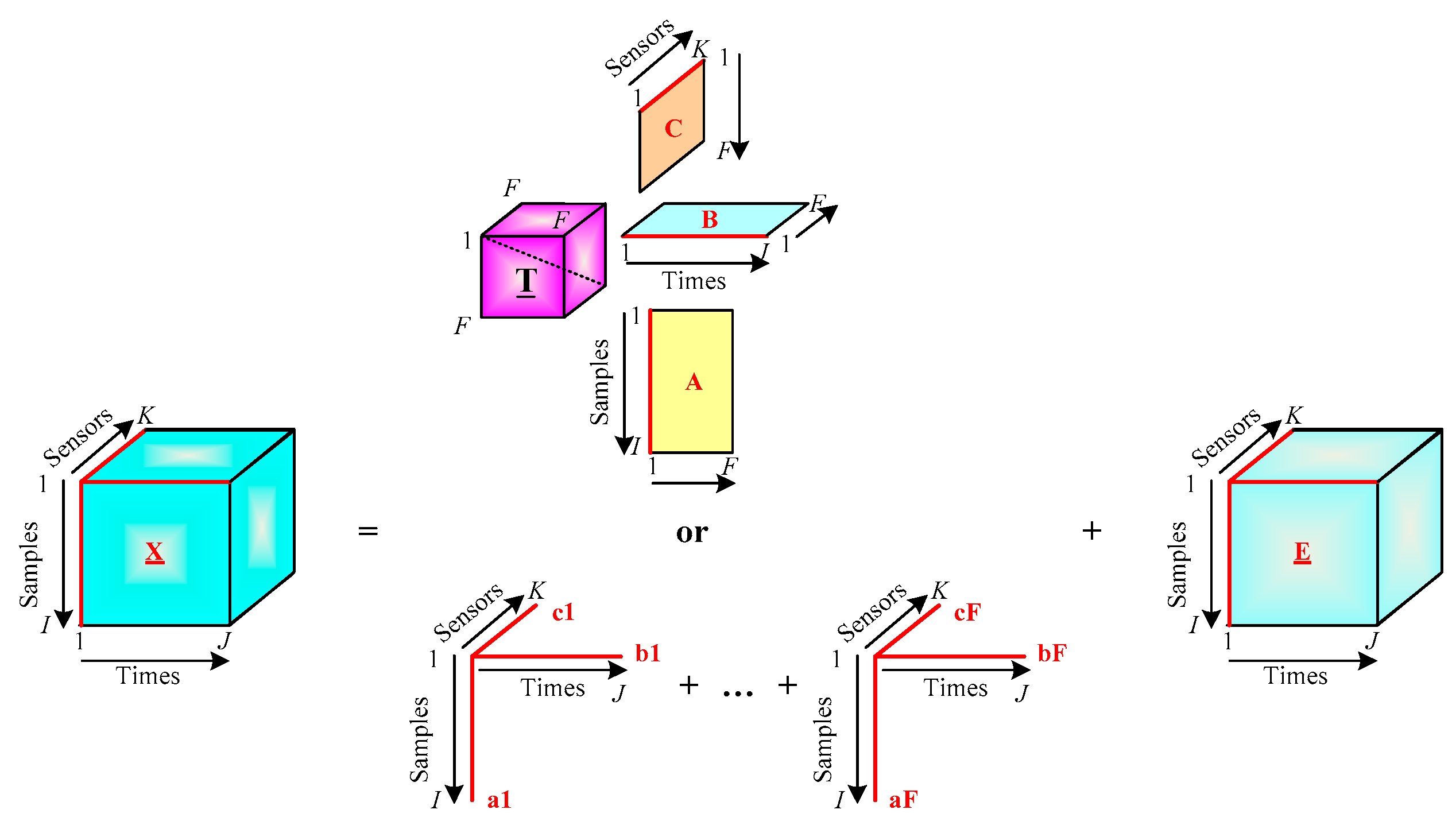
In order to build the PARAFAC model, the data array
is first arranged into a three-way array
X (
I ×
J ×
K) of three dimensions as samples × times × sensors. In order to examine whether each measurement value is indication of normal or abnormal operation, the first dimension is arranged with the 5002 measurement samples and the second dimension is only one associated with time. The third dimension is the 52 sensors, thus
X (5002 × 1 × 52) is obtained:
One element
xijk in
X corresponds to the measured sensor signal value
i at time instant
j from sensor
k. For each sensor, every sample represents a value measured at a particular time instant. The measurement data can be considered as linearly independent of each other because many processes associated with wind turbines are non-linear and measurements are made at 10 min intervals. The sensors are used to monitor different phenomena including electrical, mechanical, thermal, chemical and meteorological phenomena, which means that the components will not be highly collinear in dimension three. Thus the factors of the PARAFAC model can be uniquely determined [
18].
In order to improve the accuracy for fault detection, mean-centring is performed, which aims to remove constant terms in the dataset in order to increase the difference between the samples. Mean-centring across the first dimension (
i.e., the sample dimension) can be done by metricising the array to an
I ×
JK matrix, and then centring it in an ordinary two-way analysis [
22]:
5.2. Determining the Factors
To determine the factors, PARAFAC models with an increasing number of factors from 1 to 5 are built based on the mean-centred data. The value of the core consistency is 100%, 98%, 873.%, 44.2% and 31.7%, respectively. It is typically decreasing more or less monotonically with the number of factors, because the influence of noise and other non-trilinear variation increase with number of factors. It is found that the number of factors, which better describe the data, should be F = 3. The three-factor PARAFAC model has a core consistency of 87.3%. When the factor is over 3, it will lead to a sharp decrease in the degree of core consistency.
The PARAFAC model with F = 3 can be obtained by using ALS algorithm, as described in Equation (5). Consequently, the three loading matrices are therefore A (5002 × 3), B (1 × 3) and C (52 × 3), corresponding to the sample mode, the response mode and the sensor mode, respectively. The number of columns of the three matrices are all 3. In the subsequent sections, the different modes will be noted as follows: sample mode (A): a1, a2, a3; response mode (B): b1, b2, b3; sensor mode (C): c1, c2, c3. The sample mode and sensor mode will be illustrated with scatter loadings plots.
5.3. Fault Detection
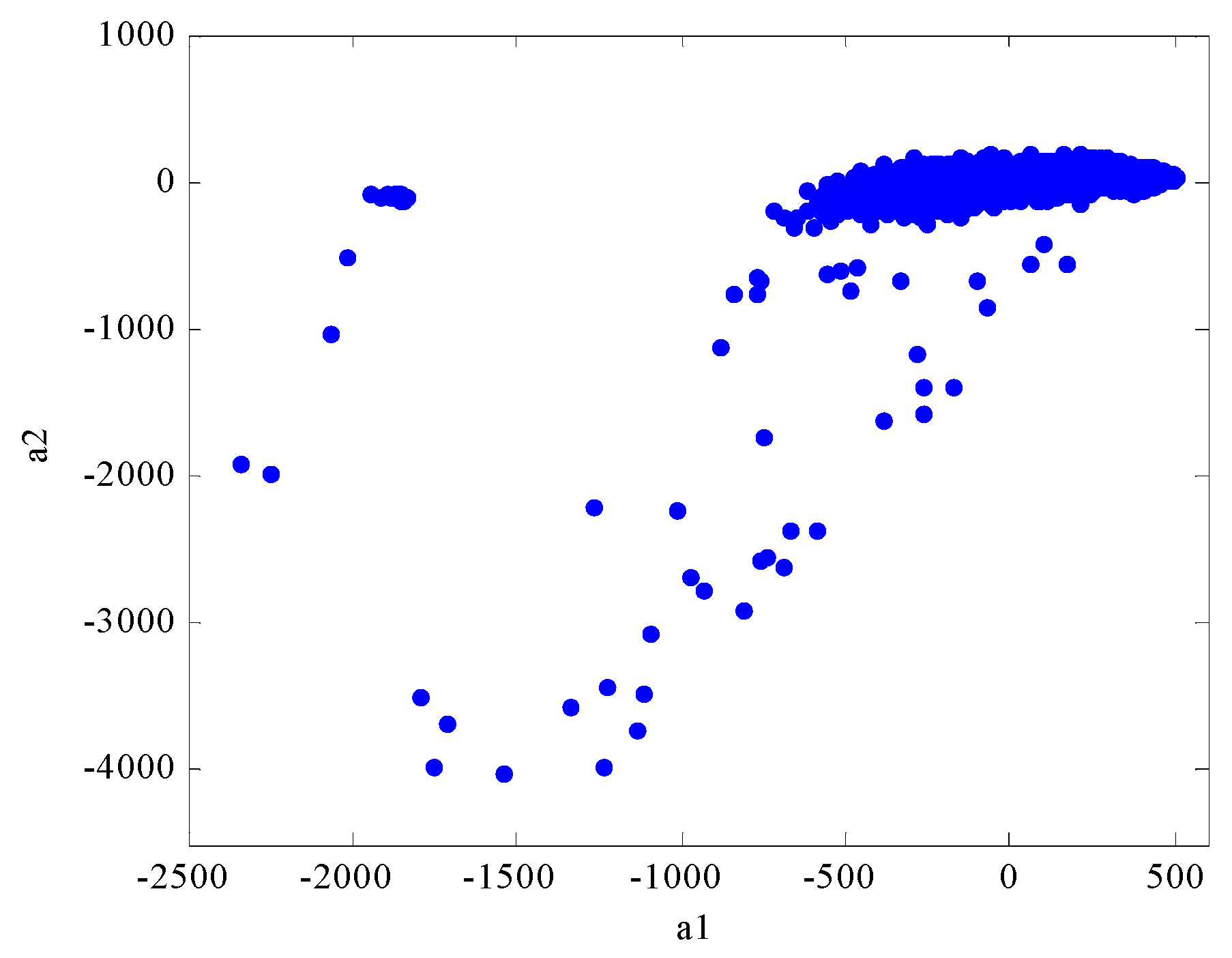
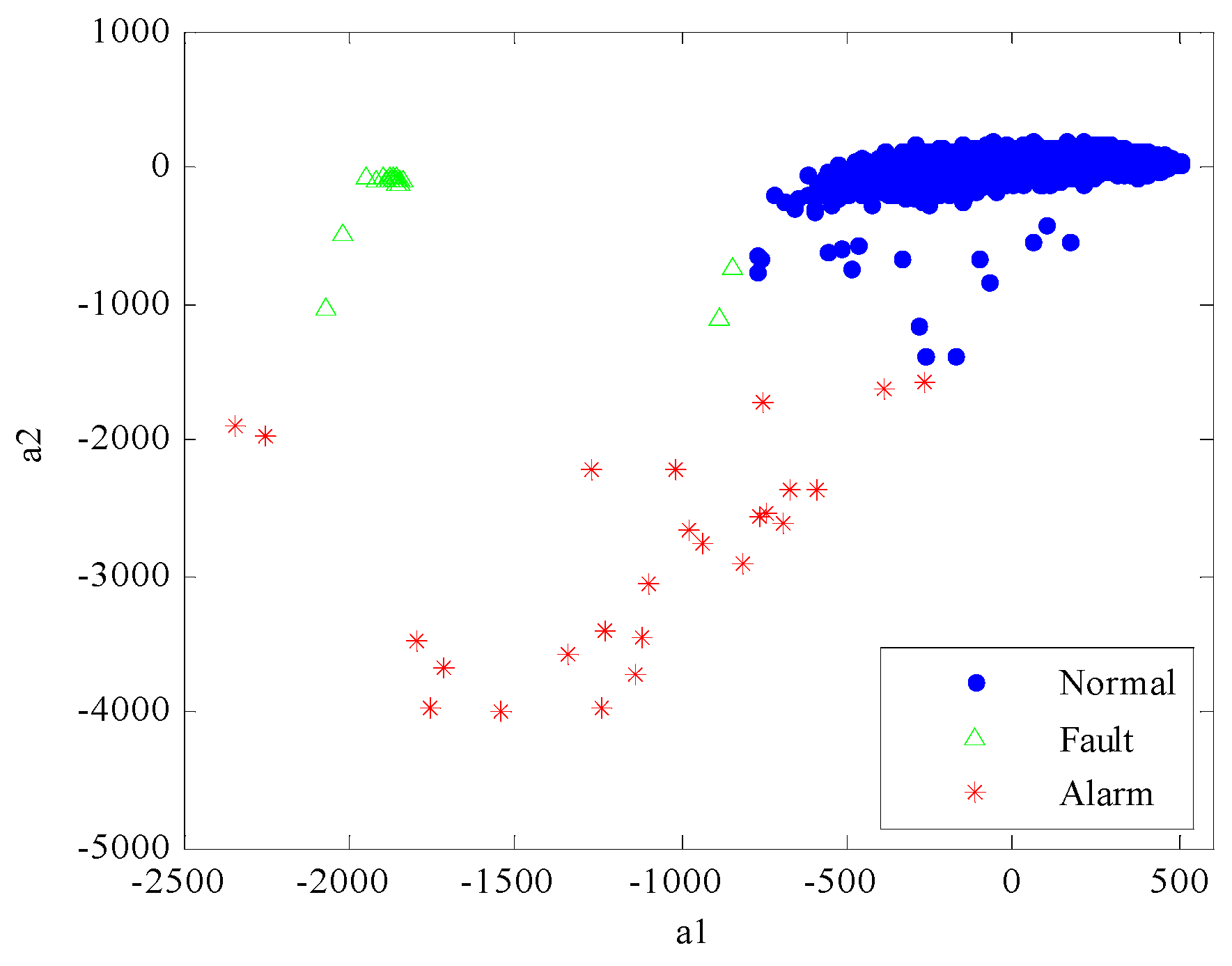
Fault detection aims to identify data patterns which do not conform to the principle of expectation. The loading plot (
Figure 4) showing correlations between the first two factors (
a1
versus a2) for the sample mode (the loading matrix
A) offers a clear way for visualising all the samples. Because mean-centring across the first dimension was done as described in Equations (10), most of measurement points are accumulated in the vicinity of the coordinate origin (0,0). Compared with
Figure 2, it can be seen that these measurement points represent normal operation of the wind turbine. Some of them are clustered in the left plot far away from the origin indicating fault conditions with a reduced active power output, while the points scattered in the lower part of the plot representing alarm conditions.
In order to verify if the extracted features by the PARAFAC model are good ones for fault detection and to find out which group each measurement point belongs to, the loading matrix
A is now analysed using
K-means clustering method.
Figure 5 shows that three types of measurement data are clearly distinguished from each other. The alarm samples distributes more dispersedly, which indicates the great variability of their measurement values.
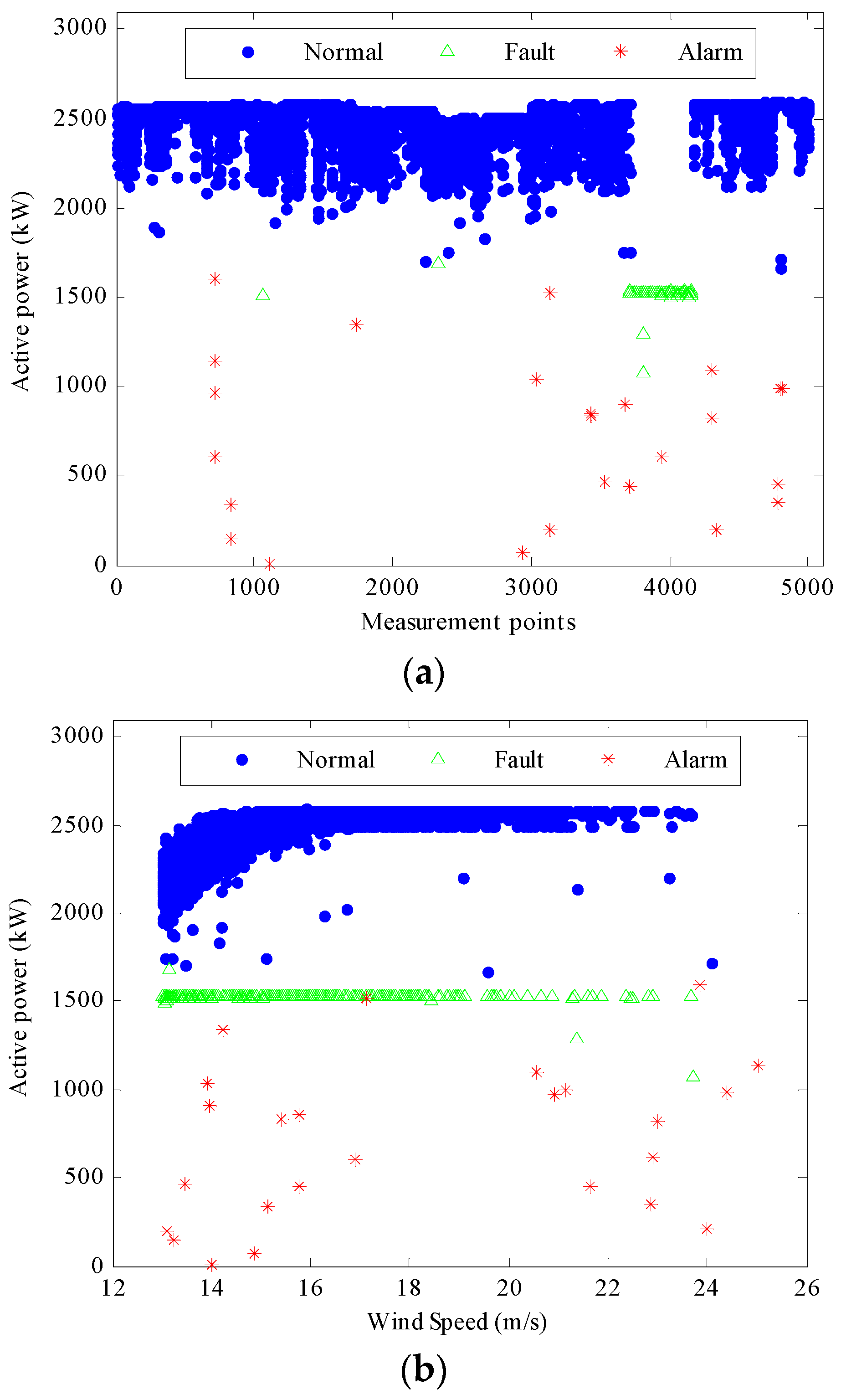
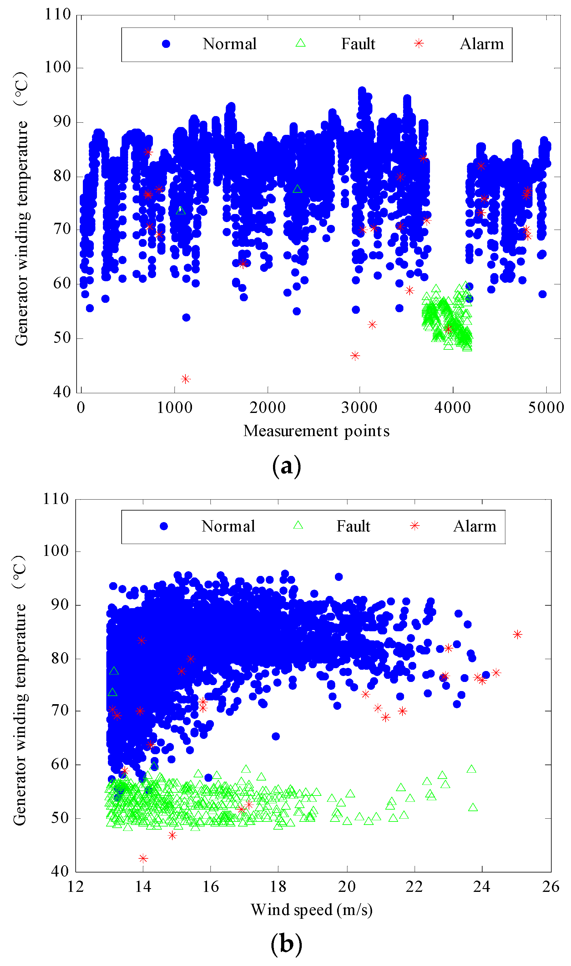
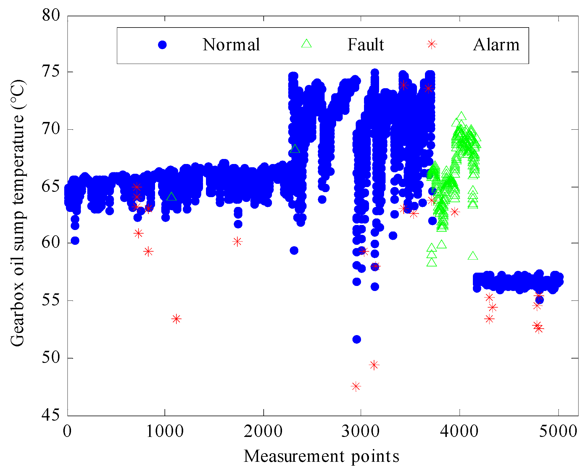
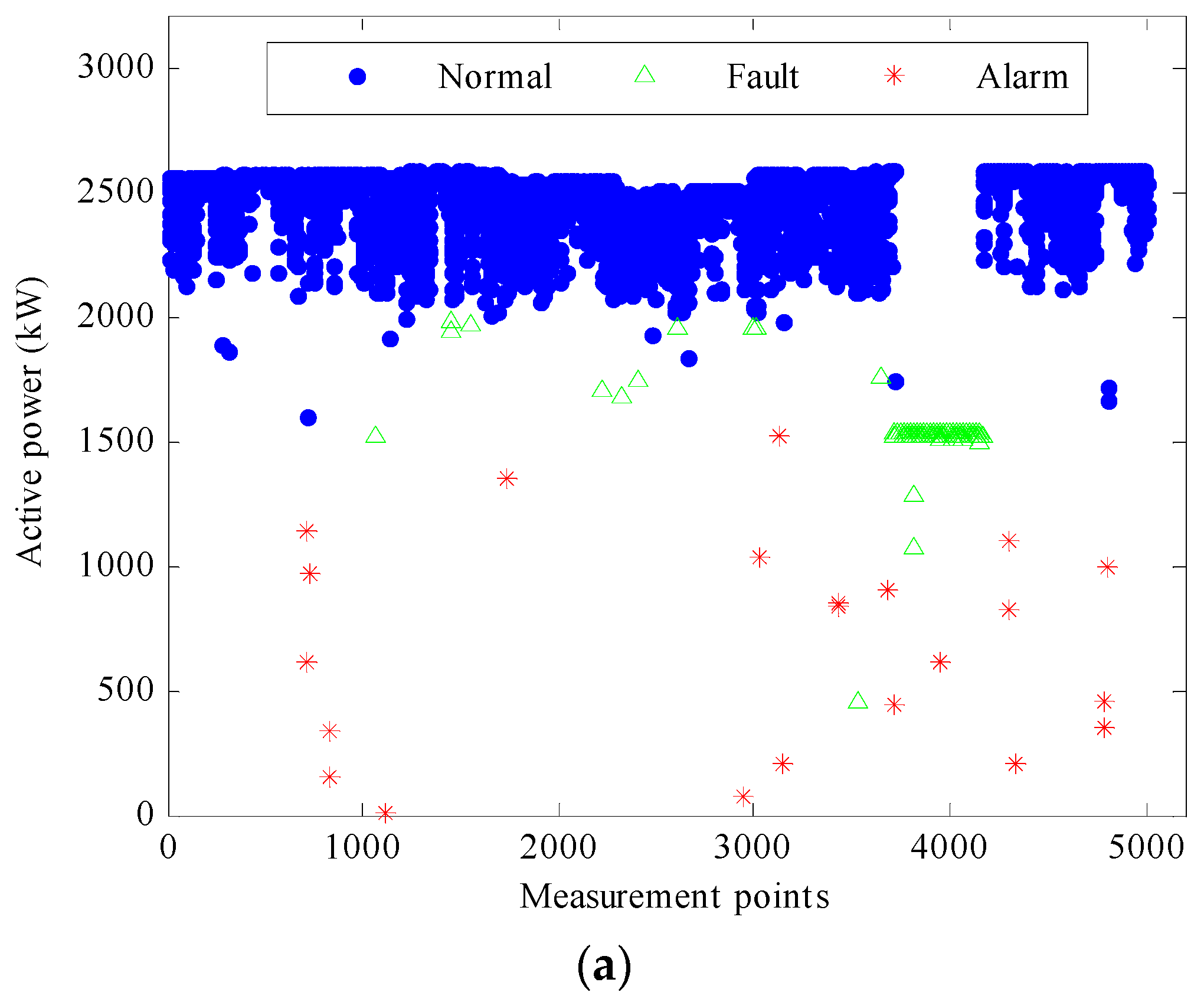
Each sample represents a value measured at a specific time, so we can know which group it belongs to. Thus the active power and the generator winding temperature can be plotted against measurement time and wind speed, as shown in
Figure 6 and
Figure 7, respectively. In these figures, the blue dots represent normal measurement points while the green triangles represent fault points, and the red stars represent alarm points. These figures indicate a clear distinction between the three operational patterns of the turbine. Having checked the alarm logs, all the measurement points for which the active power is lower than 1.5 MW while the wind speed is larger than 13 m/s are marked with red stars in
Figure 6. These figures also show several significant features, as summarised below:
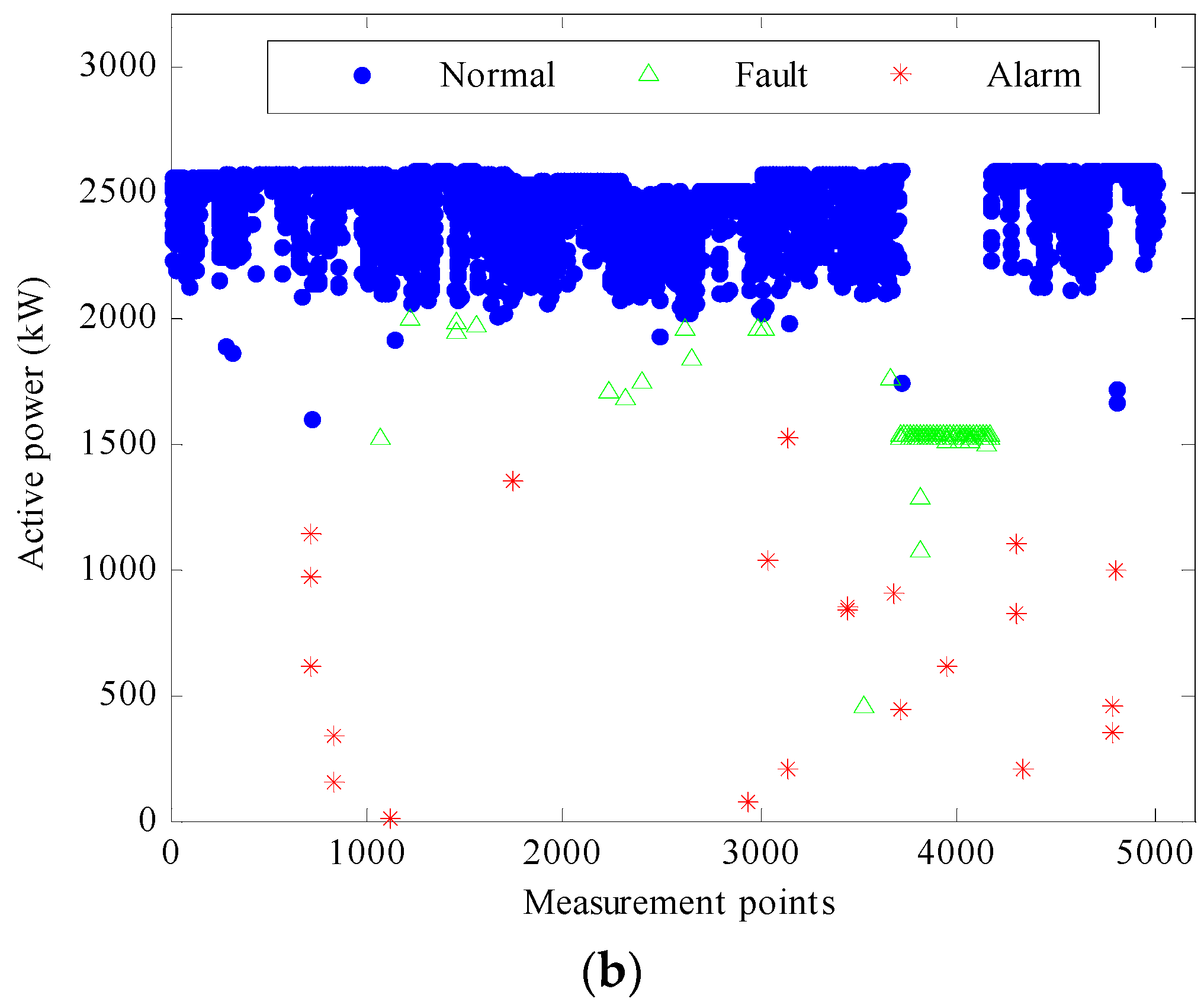
The active power normally increases with increasing wind speed until it reaches a stable value of approximately 2.5 MW. The generator winding temperature also increases with the rising wind speed.
During the fault operation period, the active power and the generator winding temperature are reduced to around 1.5 MW and 50–58 °C, respectively, despite the increase in wind speeds. This time period occurs from sample 3711 to sample 4162 for a duration of 4510 min. It was found from the alarm logs that a low gearbox oil sump temperature appears to have been the cause of the problem.
The discrete points marked as red stars in
Figure 6 indicate short excursions of the active power outside the normal range. It was found from the alarm logs that the problems were mostly associated with the wind speed which was close to the cut-out speed and with high or low gearbox oil sump temperatures.
For example, at samples 4783 and 4784, the wind speed was 22.9 and 21.7 m/s, respectively, which might be too strong for the generator and can thereby damage the turbines. Thus, the brake device has to be put in use to stop the wind turbine from running at high wind speeds. In sample 3434, the gearbox oil sump temperature reached a high value of up to 73.88 °C. In sample 2944, it was reduced to 47.52 °C. In order to ensure the safe operation of the turbine, the system automatically limits the power operation when the gearbox oil temperature is too high or too low. The discrete generator winding temperature points, as shown in
Figure 7, are also related to these wind speed and gear oil sump temperature events.
5.4. Sensor Selection
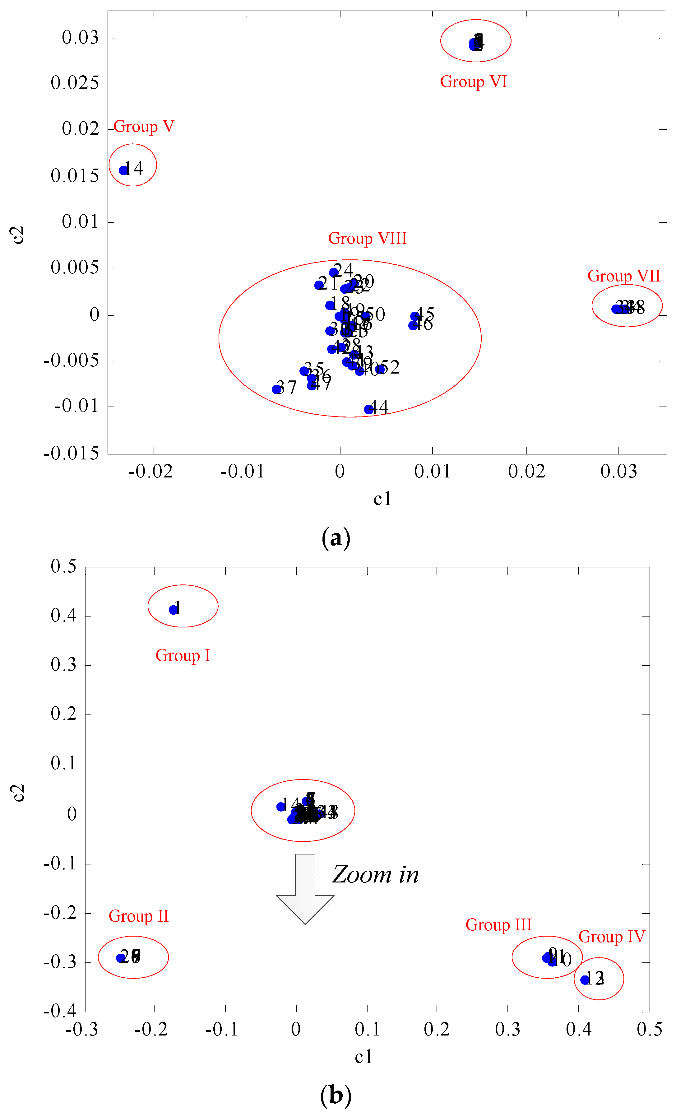
With regards to the sensor mode (the loading matrix
C which is relative to the sensor contributions), the loading plot
c1
versus c2 and an enlarged view of the central cluster are shown in
Figure 8. It can be seen that 52 sensors can be divided into eight groups, which are summarized in
Table 1. Most of the sensors (Group VIII) are concentrated in the vicinity of the coordinate origin (0,0). Sensor 1 (Group I), sensors 26–29 (Group II), sensors 9–11 (Group III), sensors 12–13 (Group IV), sensors 14 (Group V), sensors 2–8 (Group VI) and sensors 33, 34, 48 (Group VII) belong to the different groups, respectively.
The readings of the grouped sensors generally behave similar to each other and are highly correlated. Group I-VII lie in the areas far from the origin, which indicates that the response values of these sensors change notably during a fault condition. On the contrary, the signals of Group VIII changed a little, which means that the fault condition does not cause these signals to change greatly during the fault. For example, during the fault operation of the wind turbine, the active power (sensor 13) and generator winding temperature (sensor 33) decrease greatly, as shown in
Figure 6a and
Figure 7a, respectively, while the gearbox oil sump temperature (sensor 47) remained relatively constant, as shown in
Figure 9.
We can randomly choose one sensor from each respective group. Therefore under this wind turbine operation condition, the size of the sensor array can be reduced to eight by selecting sensors as shown in
Table 1. If sensors 1 (nacelle position), 2 (pitch position 1), 9 (mains current phase A), 12 (apparent power), 14 (reactive power), 26 (generator speed), 33 (temperature generator 1), 52 (temperature cooling water) are selected, the responses of these eight sensors can be used to characterize the whole sensor array response pattern under this operation condition. With the method described in
Section 5.3, the PARAFAC model of this optimised array can be obtained, and the active power output against measurement time for fault detection is plotted in
Figure 10a.
6. Conclusions
The use of PARAFAC is studied for condition monitoring of wind turbines, evaluated with SCADA data from an operational wind farm. In order to build a suitable model, the SCADA data are selected and pre-processed in order to obtain an appropriate three-way dataset. The results from the PARAFAC model show its effectiveness in providing easily interpretable plots revealing the turbine conditions. Combined with the K-means clustering method, three kinds of wind turbine operation conditions are identified, i.e., normal, fault and alarm conditions. In the meanwhile, the contribution results of the sensors are also utilized to optimise the sensor array and to reduce data redundancies between sensors. The sensors are classified into eight groups. By selecting one representative senor randomly from each group, the eight sensors are able to characterize the whole sensor array response pattern. It can be found from the loading plot for the sensor mode that there were remarkable changes in the powers, main currents, and generator winding temperatures when the turbine operated under fault conditions. However, further work remains to determine the validity of the approach, including testing the measurement data from more wind turbines. The measurements when the wind speed is relatively low (less than 13 m/s in this study) must also be considered so that results can be more robust and convincing, allowing decisions to be made for optimal maintenance scheduling.


