Intentional Islanding Algorithm for Distribution Network Based on Layered Directed Tree Model

Abstract

In this study, a novel intentional island model of a distribution system with distributed generations (DGs) is presented and the improved Dijkstra algorithm is used to solve this model. This paper abstracts the distribution network with DGs to the layered directed tree according to its radial structure and power restoration process. In consideration of grade, controllability, capacity, level and electrical betweenness of load, the model weights load and maximizes total load weight in the island. The proposed model considers power balance, node voltage, phase angle and transmission capability of the branch, and network connectivity to meet practical engineering requirements. The improved Dijkstra algorithm formulates a search rule to select the load that can be divided into an island in descending order of the shortest path between the load node and DG node. An optimal island partition scheme is achieved through three stages: origin island, baby island and mature island. Meanwhile, scheme adjustment and constraint checking are used alternately to balance objective functions and constraints. The improved IEEE 43-bus distribution network is applied to verify the validity of the algorithm. A comparison of two island methods shows that the proposed algorithm can generate a reasonable scheme for island partitioning.

1. Introduction

Distributed generation (DG) can improve energy utilization efficiency and power supply reliability. When a fault happens in a distribution network, island operation is verboten according to the initial operation requirements [1] and DG is required to quit the operation. In the distributed network with high penetration DG, the absence of the island operation will reduce the economic level of the system and the operation efficiency of the DG. According to the generation capacity of DG, the distribution network can form some local island systems to effectively restore some important loads, which improves the power supply reliability and makes full use of the DG.

In consideration of distribution network configuration, the maximum capacity of DG, load grade and size, intentional islanding makes an islanding scheme and determines a reasonable island area in advance [2,3]. When a fault happens at the upper transmission system, the island still can serve partial or full loads according to the pre-determined scheme [4,5].

The islanding scheme is a multi-objective, multi-constraint, discrete nonlinear combinatory optimization problem, and it determines the reasonable splitting point based on the network structure of the power grid and the properties of plant and load. Some researchers have done an intensive study on the transmission system islanding scheme. The ordered binary decision diagram (OBDD) –based three-phase method is proposed to search for proper splitting strategies of a large-scale power system [6,7]. Other algorithms combine slow coherency theory and the multilevel recursive bisection algorithm [8,9], and the spectral clustering method is also used to identify the coherent generators [10]. Because of the difference in network structure, the intentional islanding algorithm for a transmission system is not suitable for a distribution system. Some novel island schemes have been introduced for a distribution network. A two-state search method is proposed to minimize load loss [11], and the method uses two search processes to place the important load and general load into reasonable islands. However, the general load search process does not allow the combination of islands, and many small islands reduce the utilization of DGs. In [12], a constraint satisfaction problem (CSP)-based method is adopted to create a collection of network partitioning results with respect to individual DGs meeting the imposed network constraints; the model needs to build a constraint matrix to describe the coupling relationship between the co-domains of DGs. The computational expensive work limits its application in distribution networks with large-scale DGs. Based on the concept of source cell and load cell, a heuristic island partition algorithm to maximize weighted summation of the load cells is shown in [13]. As in [12], the algorithm only takes into account the uncontrollable load but not the controllable load, which is also called interruptible load. The graph-based search algorithm can also be used to realize island partitioning [14], and the partition result is only one island covering all DGs, and the algorithm will lose more loads in a distribution network with wide-area DGs. A novel optimum island partition model based on the tree knapsack problem (TKP) is presented in [15]. The algorithm will cause some inconvenience to power restoration, regardless of the hierarchy of load location in a distribution network. Furthermore, the normalization process in the algorithm inaccurately estimates the capacity of load and DG, which produces more load loss. In addition, these methods in [11,12,13,14,15] do not consider network loss which reduces the power that can be provided to load in an island.

An optimal islanding algorithm should consider the following factors and constraints: (1) maximizing important load and total load in an island; (2) minimizing network loss; (3) the controllability of DG and load; (4) the convenience of the power restoration. Thus, this paper proposes an intentional islanding algorithm for a distribution network based on the layered directed tree model. The layered directed tree graph is used to describe the distribution network with DGs based on its radial structure and power restoration process. Node and edge are weighted according to their operating parameters and electrical betweenness. Based on the improved Dijkstra algorithm, the intentional islanding algorithm formulates a search rule to achieve an optimal island scheme which covers more loads with high weight and has less network loss and provides more conveniences for power restoration. Plan adjustment and constraint checking are used alternately to ensure secure and stable operation for the distribution network.

The rest of the paper is arranged as follows. Section 2 introduces a layered directed tree model to express the distribution network and defines the weight of the nodes and edges. The object functions, constrained conditions and partitioning algorithm of the islanding scheme are given in Section 3. In Section 4, the method and comparative algorithms are applied to the improved IEEE 43-bus system to demonstrate the method’s validation. Section 5 provides some concluding remarks.

2. Layered Directed Tree Model

2.1. Tree Construction Method

Although the distribution network has a ring network structure, it usually runs in open-loop state and mainly uses the radial structure. Each power supply path can be considered as a tree in the radial distribution network. The tree is rooted from a source node, and it defines load and switch as the leaf mode. Then the whole distribution network can be regarded as a forest composed of this type of tree. DG only adds the special leaf node to the tree, which does not change the original structure of distribution system.

The tree made of a connected graph can be defined as a triple [16]: $T=\left(V,E,W\right)$, where $V$ is the node set, $E$ is the edge set, $W$ is the edge weight set. The distribution system with DGs is illustrated in Figure 1, and the corresponding layered directed tree is shown in Figure 2.

All island sets can be acquired though traversing all edges of the tree. For a radial distribution network with $n$ nodes and $n-1$ edges, the solution space of the islanding scheme is $2^{n-1}$, which is a terrible computation, so network simplification is essential for reducing the search space and simplifying calculations. According to system power flow, the tree is layered from the root node to the foot node, while the edge is assigned to the level of its starting node. As shown in Figure 2, the whole tree can be divided into five layers. The layered directed tree has a hierarchy and directivity; the top-down hierarchical structure simulates the power restoration sequence of the radial distribution network, and the directionality from the root node to leaf node represents the directionality of the power flow.

2.2. Special Load Node

The traditional connected graph of a distribution network generally considers load directly connected to the bus and ignores the load node located at the branch between two buses. In Figure 3a, the load L5 directly connects to the bus node Bus4, so the load node and the bus node constitute an edge. The load node located at the branch and two bus nodes at both sides of the branch constitute triangle edges, such as L6, Bus4 and Bus6 in Figure 3a. The triangle provides more path choices for the island scheme to increase the flexibility of intentional islanding.

Interruptible load (IL) is a method in which the customers sign an interruptible load contract with the utility to reduce their demand at the fixed time of system peak or any time requested by the utility [17]. It has the flexibility to choose the amount of shedding load, which contributes to expanding the island area. For a load node $L$ with $a\%$ uninterruptible parts and $b\%$ interruptible parts ($a+b=100$), a brother node with load $b\%\times P_L$ is created for node $L$, and the remaining load $a\%\times P_L$ stays with node $L$. For example, the load L9 in Figure 1 is 80 kW in which 30% is IL and 70% is conventional load. In Figure 3b, the brother node L9B with 24 kW represents the IL included in L9, which utilizes advantageous controllability of the IL. The remaining uninterruptible load can be expressed as L9A.

2.3. Connected Graph Weight

2.3.1. Node Weight

The node set can be expressed as $V=\left\{v_i|0\le i\le n-1\right\}$ where $n$ is the number of nodes including DG nodes, bus nodes and load nodes; $v_i$ is the weight of node $i$. In large complex networks, not all nodes are equivalent, and the removal of a node can have a very different effect [18]. In social network analysis, the concept “betweenness” is proposed to show the influence of a node on connectivity and anti-attacking of the network [19]. In the distribution network, electrical betweenness is used to measure the important role of a node in the network structure and in power transfer. Reference [20] shows a small number of nodes have high betweenness in the power grid, and the faults in these nodes lead to the redistribution of the shortest path between the nodes, which then triggers a system cascading failure. Therefore, the paper introduces electrical betweenness as a factor in node weight.

(a)

Bus node

The normalized weight of the bus node can be indicated as:

$$\begin{array}{l}{\mathsf{\chi }}_i={\displaystyle \sum _{k\in T}\frac{W_{k\left(i\right)}}{W_k}}\\ B_{vi}=\frac{{\mathsf{\chi }}_i}{{\mathsf{\chi }}_{\max }}\end{array}$$

(1)

where ${\mathsf{\chi }}_i$ is the weight of the bus node $i$; ${\mathsf{\chi }}_{\max }$ is the maximum weight of all bus nodes; $W_k$ is the number of shortest paths between load node $k$ and the DG node; $W_{k\left(i\right)}$ is the number of shortest paths covering bus node $i$; the shortest path is the smallest branch impedance between load node $k$ and the DG node; $B_{vi}$ is normalized weight of bus node $i$;

(b)

Load node

The weight of the load is determined by the grade, level, capacity and controllability of the load, and the controllability of the load represents whether the load is interruptible. The load with a high grade should be given priority to ensure the power supply reliability of the important load in the process of the islanding scheme. Under the same load grade, the load with a larger capacity should firstly join the island to maximize the power restoration area. Besides, dividing the load with a high level into the island is convenient for power restoration. Meanwhile, IL can greatly enhance the operation reliability of the power grid and economic benefits, so load controllability is an indispensable factor for the islanding scheme. Considering the above factors, the load weight can be expressed as:

$$\{L_{wi}={\mathsf{\lambda }}_1{L}_{Gi}+{\mathsf{\lambda }}_2{L}_{Ni}+{\mathsf{\lambda }}_3{L}_{Ci}+{\mathsf{\lambda }}_4{L}_{Ei}+{\mathsf{\lambda }}_5{L}_{Li}$$

(2)

where $i$ is the load node; $L_{wi}$ is the weight of the load node $i$; $L_{Gi}$ is the load grade of node $i$, and its range is 1, 0.1, and 0.01 which represent the first, second and third grade load; $L_{Ni}$ is the normalized capacity of load $i$; $L_{Ci}$ is the controllability of load node $i$, and $L_{Ci}=1$ represents that the load is controllable; $L_{Li}$ is the normalized level of load node $i$; $L_{Ei}$ is the normalized electrical betweenness of load node $i$. Measuring the influence of load nodes in the network, ${\mathsf{\lambda }}_1-{\mathsf{\lambda }}_5$ is the proportion of five factors, which are 0.4, 0.25, 0.15, 0.1, 0.1, respectively. In order to improve the objectivity and scientific validity of the weight coefficient, this paper combines several kinds of typical subjective weighting methods and objective weighting methods to determine the weight value of each index. The method overcomes the shortcomings of the single weighting method and makes sure the weight is more reasonable (details are available in the Appendix A1, Appendix A2, Appendix A3, Appendix A4 and Appendix A5). The method can be used to determine the weight for the latter part.

If a load $L_i$ has interruptible parts, such as L9A in Figure 3b, the method calculates weight for the interruptible load and the conventional load; then the sum of the two parts’ weights is the final weight of $L_i$.

The normalization process of load capacity can be expressed as:

$$L_{Ni}=\frac{P{L}_i}{P{L}_{\max }}$$

(3)

where $P{L}_i$ is the capacity of load node $i$; $P{L}_{\max }$ is the maximum load.

The electrical betweenness of the load is illustrated as:

$$\{\begin{array}{l}{\mathsf{\beta }}_i=\frac{1}{n{l}_i}\\ l_i={\displaystyle \sum _{i,j\in V}\frac{2d_{\min .ij}}{n(n-1)}}\end{array}$$

(4)

The normalization process of the electrical betweenness can be expressed as:

$$L_{Ei}=\frac{{\mathsf{\beta }}_i}{{\mathsf{\beta }}_{\max }}$$

(5)

where $n$ is the number of load nodes; $l_i$ is the average shortest path between node $i$ and other nodes; $d_{\min .ij}$ is the shortest path between nodes $i$ and $j$ in the network; ${\mathsf{\beta }}_i$ is the electrical betweenness of load node $i$; ${\mathsf{\beta }}_{\max }$ is the maximum electrical betweenness of the load.

The normalization process of the load level can be expressed as:

$$L_{Li}=\frac{L{L}_i}{L{L}_{\max }}$$

(6)

where $L{L}_i$ is the level of the load node $i$; $L{L}_{\max }$ is the maximum load level.

(c)

DG node

The weight of the DG node can be written as:

$$G_{wj}={\mathsf{o}}_1{G}_{Nj}+{\mathsf{o}}_2{G}_{Rj}+{\mathsf{o}}_3{G}_{Cj}$$

(7)

where $j$ is the DG node; $G_{wj}$ is the weight of DG node $j$; $G_{Nj}$ is the normalized capacity of DG node $j$; $G_{Rj}$ is the reactive power supporting the capability of DG node $j$; $G_{Cj}$ is the controllability parameter of DG node $j$; ${\mathsf{o}}_1-{\mathsf{o}}_3$ is the proportion of three factors, which are 0.7, 0.2 and 0.1, respectively.

The normalization process of DG capacity can be expressed as:

$$G_{Nj}=\frac{P_{Gj}}{P_{G\max }}$$

(8)

where $P_{Gj}$ is the rated power of DG; $P_{G\max }$ is the maximum rated power of DG.

The reactive power supporting capability of DG is crucial for voltage stability in the island system. The reactive power regulating range of Doubly-Fed Induction Generator (DFIG) depends on the active power of the stator winding. For inverter-distributed generation (IDG), such as fuel cell (FC), photovoltaic (PV) and microturbine (MT), their active power affects the regulating range. Diesel generation (DEG) can regulate the synchronous generator excitation flux to control the reactive power. Thus, the reactive power supporting capability of DEG is most efficient in all DGs, so $G_R=0.99$ for DEG. With the same active power, the reactive power adjustment range of DFIG is wider than IDG [21], so $G_R=0.66$ for DFIG and $G_R=0.33$ for IDG. The controllability of DG represents its ability to regulate output power according to the dispatching order. DFIG and PV are greatly influenced by the natural environment and cannot regulate the active power according to load fluctuation, which has a worse controllability, so $G_C=0.5$. In the allowable capacity range, DEG and MT can regulate the output power to make up the power balance, which has a better controllability, so $G_C=1$.

2.3.2. Edge Weight

The edge set covers three kinds of edges: the edge consisting of the bus node and load node, the edge consisting of the bus node and DG node, and the edge consisting of the bus nodes. The edge set and weight set can be expressed as:

$$\{\begin{array}{l}E=\left\{e_{ij}|0\le i,j\le n-1,i\ne j\right\}\\ W=\left\{w_{ij}|0\le i,j\le n-1,i\ne j\right\}\end{array}$$

(9)

where $w_{ij}$ is the edge weight, whose value represents the importance and priority of the edge in the process of the islanding scheme. Details of the weight determination are as follows:

(a)

The edge consisting of the bus node and load node:

$$W=a{L}_{wi}+\left(1-a\right)Z_{Ni}$$

(10)

where $i$ is the load node; $L_{wi}$ is the weight of load node $i$; $Z_{Ni}$ is the normalized edge impedance; $a$ is a factor, and its value is 0.8.

The standardization process of edge impedance can be expressed as:

$$Z_{Ni}=\frac{Z_{\max }-Z_i}{Z_{\max }-Z_{\min }}$$

(11)

where $Z_i$ is the impedance of the edge consisting of the bus node and load node $i$; $Z_{\max }$ is the maximum edge impedance; $Z_{\min }$ is the minimum edge impedance.

(b)

The edge consisting of the bus node and DG node:

$$W=b{G}_{wj}+\left(1-b\right)Z_{Nj}$$

(12)

where $j$ is the DG node; $G_{wj}$ is weight of DG node $j$; $G_{Nj}$ is the normalized capacity of DG node $j$; $Z_{Nj}$ is the normalized edge impedance, and it can be calculated according to Equation (11); $b$ is a coefficient, and its value is 0.8.

If DG and load are at the same node, the node is considered a DG node.

(c)

The edge consisting of bus nodes:

$$W=c(B_{vm}+B_{vn})+(1-c)C{o}_{mn}$$

(13)

where $B_{vm}$ and $B_{vn}$ are the weight of bus nodes $m,n$, respectively; $c$ is a coefficient, and it is 0.4; $C{o}_{mn}$ is the priority of the edge between node $m,n$, and details of its value determination are as follows:

Case A: The edge contains a tie switch. $C{o}_{mn}$ is defined as 0.25, and the highest priority ensures the edge preferentially to join the island, which contributes to achieving the island combination.

Case B: The edge does not contain the transformer and load. $C{o}_{mn}$ is defined as 0.75.

Case C: The edge contains the transformer. Due to power loss of the transformer, the edge in case B is chosen preferentially in the process of the islanding scheme instead of case C, so $C{o}_{mn}$ of the edge in case C should be smaller than in case B. If the transformer is a three-winding transformer, $C{o}_{mn}$ is defined as 0.5. Considering the work efficiency of a three-winding transformer is higher than a double-winding transformer, the three-winding transformer can be split to two double-winding transformers, and the related $C{o}_{mn}$ is defined as 0.25.

Case D: The edge contains the load. Based on the analysis in part B of this section, the edge should be translated to three edges. The edge consisting of the two bus nodes defines $C{o}_{mn}$ according to case B; the other two edges consisting of the bus node and load node define $C{o}_{mn}$ according to Equation (10).

3. Islanding Scheme Model

3.1. Objective Function

When a fault happens, intentional islanding makes the supply of important load a top priority to reduce outage costs and restore the general loads’ power as much as possible while meeting the constraint that the total load shall not exceed the generation capacity of DGs. In addition, because of the limited capacity of DG, it is necessary to reduce the network loss for maximizing power that can be provided to loads. After the fault is cleared, the upstream system restores the power supply of the distribution network from top to bottom. The system firstly restores the loads directly connected to the root node of the distribution network, then the loads in the island connect to the distribution network, and finally other loads can be restored. To restore power conveniently, the island should cover load nodes which are as far away from the root node as possible, and the scilicet covers the high-level nodes as much as possible. Considering the three optimal objects, the objective function can be defined as:

$$\max {\displaystyle \sum \left({\mathsf{\lambda }}_1{f}_1+{\mathsf{\lambda }}_2/f_2+{\mathsf{\lambda }}_3{f}_3\right)}$$

(14)

where $f_1$ is the total load weight in the island; $f_2$ is the total network loss of the island system; $f_3$ is the total load level in the island system; ${\mathsf{\lambda }}_1$, ${\mathsf{\lambda }}_2$ and ${\mathsf{\lambda }}_3$ are weight factors, which are 10, 5 and 2, respectively.

$$\{\begin{array}{l}{f}_1={\displaystyle \sum _{i\in M}{\mathsf{\gamma }}_i{L}_{wi}}\\ {\displaystyle \sum _{i\in M}{P}_{Gi}}\ge {\displaystyle \sum _{i\in M}{P}_{Li}}\end{array}$$

(15)

where ${\mathsf{\gamma }}_i$ is a binary variable denoting that island $M$ covers load node $i$; $L_{wi}$ is the weight of load node $i$; ${\displaystyle \sum _{i\in M}{P}_{Gi}}$ is the total power generating capacity of DG in island $M$; ${\displaystyle \sum _{i\in M}{P}_{Li}}$ is the total load in island $M$.

$$f_2={\displaystyle \sum _{i\in M}{R}_i\times \frac{P_i^2+Q_i^2}{{\left|V_i\right|}^2}\times {\mathsf{\chi }}_i}$$

(16)

where $R_i$ is the resistance of branch $i$; $P_i$, $Q_i$, and $\left|V_i\right|$ are active power, reactive power, and voltage amplitude of branch $i$, respectively; ${\mathsf{\chi }}_i$ is a binary variable denoting island $M$ covers branch $i$.

$$f_3={\displaystyle \sum _{i\in M}leve{l}_i}$$

(17)

$$\{\begin{array}{l}i\in M\cap j\notin M\\ leve{l}_i\ge leve{l}_j\end{array}$$

(18)

where $leve{l}_i$ and $leve{l}_j$ are the levels of node $i$ and $j$, respectively. Equation (18) represents that the node in the island has a higher level than the node outside the island.

3.2. Constraint Condition

3.2.1. Power Balance Constraints

$$\{\begin{array}{l}{P}_{Gi}-P_{Li}=U_i{\displaystyle \sum _{j=1}^n{U}_j\left(G_{ij}\cos {\mathsf{\theta }}_{ij}+B_{ij}\sin {\mathsf{\theta }}_{ij}\right)}\\ Q_{Gi}-Q_{Li}=U_i{\displaystyle \sum _{j=1}^n{U}_j\left(G_{ij}\sin {\mathsf{\theta }}_{ij}+B_{ij}\cos {\mathsf{\theta }}_{ij}\right)}\end{array}$$

(19)

where $P_{Gi}$ and $Q_{Gi}$ are the injection active and reactive power of DG at node $i$; $P_{Li}$ and $Q_{Li}$ are the active and reactive power need of node $i$; $U_i$ and $U_j$ are the node voltages at both ends of branch $ij$; $G_{ij}$ and $B_{ij}$ are the conductance and susceptance of branch $ij$; ${\mathsf{\theta }}_{ij}$ is the phase angle difference between node $i$ and node $j$.

3.2.2. Static Security Constraint

Node voltage constraint:

$$U^{-}\le U_i\le U^{+}$$

(20)

Branch capacity constraint:

$$S^{-}\le S_i\le S^{+}$$

(21)

Phase angle difference constraints:

$${{\mathsf{\theta }}_{ij}}^{-}\le {\mathsf{\theta }}_{ij}\le {{\mathsf{\theta }}_{ij}}^{+}$$

(22)

where $U^{+}$ and $U^{-}$ are the upper and lower limits of the node voltage; $S^{+}$ and $S^{-}$ are the upper and lower limits of the branch capacity; ${{\mathsf{\theta }}_{ij}}^{+}$ and ${{\mathsf{\theta }}_{ij}}^{-}$ are the upper and lower limits of the phase angle difference between node $i$ and node $j$.

3.2.3. Network Structure Constraint

The DGs must stay connected to loads in each island, and the distributed network should keep a radial structure:

$$\forall G_i\in M_j,\exists L_k\in M_j\to \mathsf{\chi }(G_i,L_k)=1$$

(23)

where $G$ is the DG node; $L$ is the load node; $M$ is an island; $\mathsf{\chi }(G_i,L_k)=1$ shows a connected path exists between $G_i$ and $L_k$.

$$m=n-1$$

(24)

where $n$ is the number of nodes; $m$ is the number of edges.

3.3. Islanding Scheme Algorithm

According to the weight of the edge, the improved Dijkstra algorithm is applied to search for each shortest path between DG nodes and load nodes. Then the islanding scheme algorithm builds the corresponding minimum spanning tree in every island, and further completes the island combination. In the process of the islanding scheme, scheme adjustment and constraint checking are used alternately to balance objective function and constraints. The details of the island partition algorithm are shown as:

(1) Build a tree model. Based on the tree construction method described in Section 2.1, a layered directed tree is formed, and its root is the first node in the downstream area of the fault location. From the root node, bus nodes are divided into different layers along the power flow direction. Meanwhile, the DG node and load node connected to the bus are integrated in the corresponding layer. The interruptible and uninterruptable parts in the load are divided into two separate nodes according to the method in Section 2.2.

(2) Weight node and edge. According to the model proposed in Section 2.3, the weight of the bus node, load node and DG node can be calculated. The weights of edges consisting of different nodes are also introduced in Section 2.3. The progress takes into account the level, grade, size, controllability, and importance degree of the load. Controllability and rated capacity are considered to weight DG and the influence of the bus node is analyzed. In addition, the transformer and switch on the edge are covered in the analysis.

(3) Search for the shortest path. After traversing the entire connected graph, the improved Dijkstra algorithm is applied to search for each shortest path between the bus nodes; the shortest path is equivalent to the maximal sum of the edge weight. The progress builds a $n\times n$ matrix $S$, $n$ is the number of bus nodes. $S_{ij}$ is the shortest path between bus nodes $i$ and $j$. During the search, $\#$ is used to mark the bus node connecting to the DG node and $*$ is used to mark the bus node connecting to the load. For example, $S_{ij}^{\#*}$ illustrates that there exists DG at bus node $i$ and load at bus node $j$. The elements with marks $*$ and $\#$ in $S$ can be used to build a $l\times k$ matrix $T$, where $l$ and $k$ are the number of DGs and loads, respectively. $T_{\mathsf{\alpha }\mathsf{\beta }}$ is the shortest path between the DG node $\mathsf{\alpha }$ and load node $\mathsf{\beta }$.

(4) Divide the original island. Based on matrix $S$, the algorithm connects other buses to the bus directly connected to DG in descending order according to the shortest path between the bus nodes. If DG $\mathsf{\alpha }$ is at the bus node $i$, the $i\text{th}$row elements in $S$ are sorted in descending order. The $\mathsf{\nu }$ top-ranked elements in the $i\text{th}$ row and bus node directly connected to DG form the original island $O_{\mathsf{\alpha }}$. $\mathsf{\nu }$ is a quarter of the total number of buses for accelerating the island partition speed. The progress is applied to all DGs and forms $l$ original island $O_1\dots O_l$, where each original island consists of one DG and $\mathsf{\nu }$ buses.

(5) Build the minimum spanning tree. In the original island $O_{\mathsf{\alpha }}$, the algorithm adds load in descending order according to the shortest path between the load node and DG $\mathsf{\alpha }$. The objective function $f_1$ in Equation (16) promotes the load with a larger weight into the minimum spanning tree, such as the first grade load, second grade load, interruptible load and so on. As to the uncontrollable parts in the load, the algorithm reasonably sheds it to reduce network loss $f_2$. Meanwhile, static security constraints are checked, and the 10% off-limits are allowable to ensure that more loads can be divided into the island which provides more alternative schemes for the island combination. The load level $f_3$ has less portions in Equation (16), so it mainly affects third grade load. The algorithm gives preference to the load located at high levels to facilitate power restoration after the fault is cleared. This process generates the minimum spanning tree, which is also called the baby island. Then the algorithm traverses all DGs until all original islands generate the corresponding minimum spanning tree.

(6) Apply the island combination. When the baby load is small, there is power inequality between islands. Some island has redundant power whereas, because of power shortages, other islands have to cut off loads with high weights. If multiple islands have intersection, the overlapping load is double-counted, which reduces the DG utilization, so the island combination becomes an essential step.

<1> If two baby islands have overlapping loads, then the union set of islands is calculated, while the power balance constraints, static security constraints and network structure constraints are checked. ① If the island is within the constraints, the algorithm continues to search loads around the island. The loads can be added to the island until the system is beyond constraints; ② if the island is beyond the constraints, the loads with lower weight, such as the interruptible load and low grade load, should be shed to ensure the system’s normal operation.

<2> Two baby islands are neighbors. ① Only one path links the two islands and the islands can be merged along the path, while the loads at and around the path are integrated into a new island within the constraints; ② multiple paths exist between the islands. The path with the biggest weight can be selected as the connecting line. The island algorithm searches for the first grade load and second grade load around the island, and cuts off some loads with a lower weight in the island to help the high grade load join the island. If the total load weight has less improvement and the network loss has larger growth, the island combination should be stopped. In addition, as many loads with low levels as possible can be shed.

<3> The island combination in <1> and <2> enlarges the island region, so there is a probability of further island combination. The algorithm determines whether island combination is feasible according to objective function. By the time, network loss and power restoration conveniences become the uppermost restrictive factors.

<4> Finally, the bus without a connection to the load and DG is removed to complete the islanding scheme.

4. Study Case

As shown in Figure 4, the case employs an improved IEEE 43-bus system integrated with five DGs. The specific parameters of the line can be queried in reference [22], and the customized parameters of DG and load are listed in

Table 1. Distributed generation (DG) characteristics and weight of each node.

Name	Node Number	Active Power/kW	Power Type	Weight
DG1	9	25	DEG	0.639
DG2	19	100	DFIG	0.882
DG3	39	50	MT	0.516
DG4	30	100	DFIG	0.882
DG5	35	75	PV	0.641
DG6	13	75	PV	0.641

and

Table 2. Load characteristics and weight of each node.

Node Number	Active Power/kW	Load Grade	Proportion of IL	Load Weight
3	30	1	0	0.7221
4	25	2	15%	0.5171
5	10	3	0	0.1707
6	5	3	10%	0.1691
7	10	3	0	0.1418
8	5	3	0	0.1673
10	10	1	0	0.6066
11	4	2	0	0.4868
12	10	3	0	0.1586
14	5	3	0	0.1267
15	50	1	0	0.8211
16	10	3	50%	0.2799
17	10	3	80%	0.2870
18	15	3	0	0.2209
20	10	3	0	0.1781
22	35	1	0	0.7522
24	5	3	0	0.1732
26	20	2	0	0.4367
27	10	3	80%	0.3087
30	10	3	30%	0.2695
31	10	3	10%	0.1824
32	40	1	0	0.7873
33	10	2	0	0.3454
34	15	3	20%	0.2316
35	20	2	0	0.4639
36	20	3	100%	0.3711
38	15	2	0	0.3505
40	50	2	40%	0.4803
41	20	1	0	0.6394
42	20	3	10%	0.2330
43	25	3	0	0.2451

. The test system adopts reactive local compensation, so it does not concern reactive power and ignores the reactive power parameters of load and DG.

As is shown in Figure 4, when a fault happens in the upper system, Bus1 is removed, so the distribution system disconnects with the transmission system. According to the islanding scheme algorithm proposed in the paper, the island partition procedures and results are presented as follows.

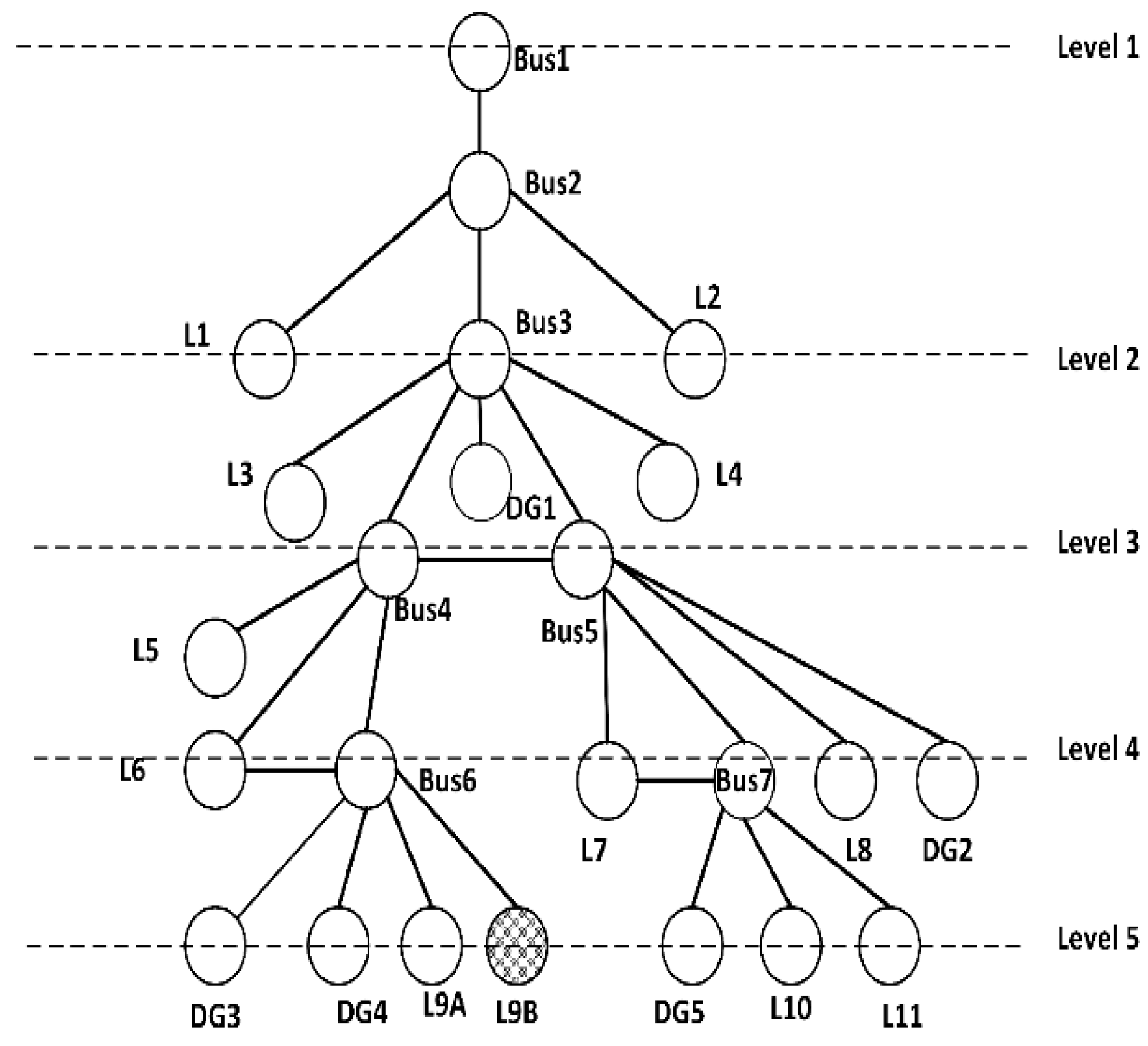
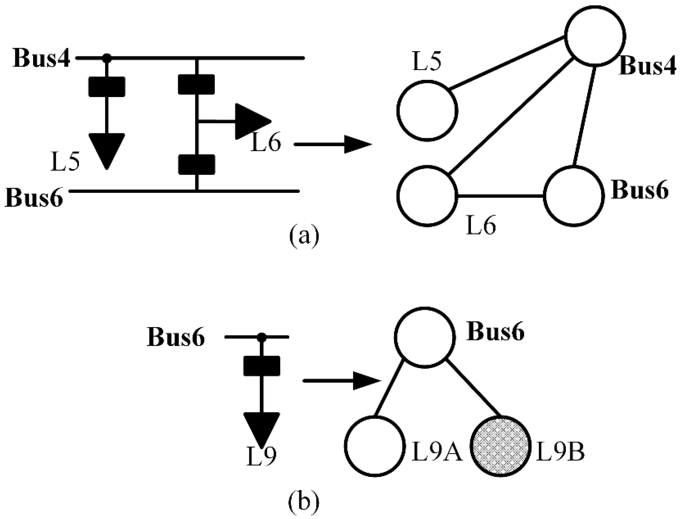
1. The layered directed tree model for the IEEE 43-bus improved test system is shown in Figure 5a. The tree has nine levels and mainly represents bus nodes; the DG and load nodes can be added to the tree according to the single line diagram shown in Figure 4. The weight of the DG and load nodes is calculated and listed in Table 1 and Table 2. The bus node contains nodes 1, 2, 21, 23, 25, 28, 29 and 37, whose weights are 0.378, 1.000, 0.719, 0.847, 0.758, 0.784, 0.912 and 0.241, respectively. According to the weight method described in Section 2.3, the algorithm calculates the edge weight of the 41 branches in the layered directed tree, and

Table 3. Weight of 43 edges.

Branch	1–2	2–5	2–6	2–15	4–3	5–7	5–8	6–12
Weight	1.064	0.834	0.826	0.964	0.619	0.156	0.169	0.164
Branch	7–17	8–9	8–23	9–16	9–10	10–11	13–4	13–18
Weight	0.214	0.951	0.814	1.063	1.390	0.392	1.101	1.005
Branch	15–19	15–20	15–28	17–10	19–22	21–24	22–26	23–29
Weight	1.750	0.499	0.905	0.446	1.681	0.409	0.479	1.336
Branch	25–13	25–27	28–39	29–21	29–25	29–30	29–37	30–32
Weight	0.863	0.917	0.844	1.207	1.307	0.932	1.031	1.716
Branch	30–38	30–40	37–31	38–33	38–34	38–35	38–36	39–41
Weight	1.797	1.409	0.239	0.248	0.241	1.035	0.311	1.349
Branch	39–43	40–42	43–14
Weight	0.954	0.356	0.186

shows the calculated results.

2. Search the shortest paths between the bus nodes and DG nodes; O1–O6 are the six original islands that form, and every island contains one DG and 10 bus nodes. The O1 has an isolated domain in which the bus nodes are exclusive and around DG1. O2 and O3 share nodes 1, 2, 15, 19, 20 and 28, and the larger shared region contributes to merging the island. Like DG1, DG2 is surrounded by bus nodes, and there are fewer nodes around DG3, so O3 extends to the region of O2 along the branch of 39–28 and presents a dumbbell shape. DG4 and DG5 are neighbor DG nodes, so O4 and O5 have an overlapping region which has potential for island combination. DG6 is located at the end-point of the network and O6 collects bus nodes in the descending order of the shortest path, so it forms the hierarchical island while O6 also shares nodes 1 and 24 with O4. The bus nodes 2, 23 and 29 have larger electrical betweenness, which shows their important role in the network structure and power transfer of the distribution network, so these nodes are divided into original islands preferentially.

The dividing procedure is illustrated in Figure 5b.

3. The minimum spanning tree T1 is based on O1 and composed of DG1 and load nodes 16–17 and 10–11. In O1, DEG has larger reactive power supporting capability and more controllability. The loads at nodes 16 and 17 have higher load grade, and loads 10 and 11 have larger interruptible load proportions. In consideration of load weight maximization, these loads have priority for being divided into the minimum spanning tree. Node 5 is a third grade load and is located at the first layer; T1 does not cover it considering the convenience of power restoration and load level maximization. Like load 5, load 17 is located at the first layer, but the advantage of 8 kW IL prompts it to integrate into T1.

4. The tree T2 is based on O2 and composed of DG2 and load nodes 15 and 22. The load nodes 15 and 22 are all first grade loads, and should show preference to the power supply. The sum load of 15 and 22 is 85 kW, so the surplus power in T2 is 15 kW. The loads at 22 and 26 have no controllable parts, which decreases the island’s capacity for the uncertainty and volatility of the DG output. Because load 22 is 20 kW, the surplus power cannot meet the load demand. The model takes interruptible load and load level into consideration, so load 26 has a lesser load weight. According to the objective functions, the lesser load weight results in load 26 being outside the island.

5. The tree T3 is based on O3 and composed of DG3 and load nodes 14, 41 and 43. Load 41 has the first grade, so the island algorithm firstly divides the load into T3. MT has more controllability and can regulate output power to rated power. After meeting the two loads, the algorithm continues to search some loads until the loads and DG3 are matching in production and consumption of power. T3 narrows the scope of O3 and cuts out overlapping parts between O2 and O3.

6. The tree T4 is based on O4 and composed of DG4 and load nodes 30, 32, 38 and 40. Load 32 is a first grade load and loads 38 and 40 are second grade loads. These loads play an important role in the power grid, and therefore need uninterrupted, reliable flows of energy in order to guarantee electricity to the masses. Load 30 should be selected to ensure the connectivity of the island. The total load is 115 kW, which seemingly exceeds the maximum supply capability of DG4, but nodes 30 and 40 have interruptible load, and 23 kW interruptible loads can be shed when DG fails to provide adequate power. The approach increases the power supply reliability of the system and realizes the economical operation of the DG. In addition, load 38 has larger electrical betweenness, so it has a higher importance degree in the distribution network, which increases the load weight and priority to be restored. Then the load at node 38 is an intersection between T4 and T5, so DG5 also can provide some power to the load at node 38. Compared to PV, the DFIG has higher reactive power supporting capability and can ensure the voltage stability of the island. In addition, DG4 has 100 kW which is larger than the 75 kW of DG5. Based on the higher reactive power supporting capability and larger capacity, DG4 will have the larger weight. The larger weight can increase the total weight of the shortest path between DG4 and the load nodes, which is beneficial for attracting the load in the island partition progress, so the first grade load at node 32 and the second grade load at node 40 are divided into T4.

7. The tree T5 is based on O5 and composed of DG5 and load nodes 33–36 and 38. All of nodes 31, 34, 36, and 42 belong to the third grade load, so loads 35 and 33 firstly joint into T5, with a second grade. In consideration of load level, load 31 is located at the sixth level and the level of load 34, 36, and 42 is eight. In order to successfully restore power, the distribution network tends to select the load with the higher level. The interruptible parts of load 42 are 2 kW, and interruptible loads also possess 3 kW and 20 kW in loads 34 and 36, respectively. At the end, loads 34 and 36 are divided into T5, and nodes 31 and 42 suffer complete power outage. The difference illustrates that the grade, capacity, and controllability of load will have great influence on the islanding scheme.

8. The tree T6 is based on S6 and composed of DG6 and load nodes 3, 4, 18 and 27. Load 18 has a larger weight than 24, so T6 excludes load 24. The output of DG6 is greatly influenced by the natural environment including as temperature and light intensity. The IL can be regulated to maintain power balance.

Nodes 3–8 are the forming progress of six baby islands as shown in Figure 5c.

9. Mature island M2 aggregates baby islands T2 and T3. In T2, the idle 15 kW reduces the utilization of DG2; in addition, the second grade load 26 may suffer a power break. The island combination can reasonably integrate T2 and T3 as one unity and regulates the supply-demand relationship between DG and load to achieve the objective function. At first node 14 is divided into T3, then it is cut off to ensure the priority of power supply to node 26 with high betweenness, in the progress of island combination.

10. Mature island M3 is a combination between T4 and T5. The sum of load in T4 and T5 is 180 kW in which the interruptible load is 26 kW, and the total output of DG4 and DG5 is 175 kW. The controllable load at nodes 30 and 34 can be shed to keep power balance.

11. Mature islands M1 and M4 are baby loads T1 and T6, respectively. In mature island M1, DG1 consisting of DEG has stronger generation controllability; in addition, ILs exist at nodes 16 and 17, and the island system can flexibly control the amount of generation and consumption to achieve high quality power supply. In M4, the further combination between mature island M3 and M4 is prevented by higher network losses and the loads with high betweenness are curtailed.

Nodes 9–11 are the island combination progress shown in Figure 5d.

12. The island algorithm should check static security in the progress of island combination. Let DG1 (DEG) and DG3 (MT) export rated power. As intermittent DG, DFIG and PV use the probability model to simulate output power influenced by the natural environment [23,24]. The algorithm performs stochastic load flow calculations to check whether the island is beyond system static security constraints. The analyzed result shows that the probability of overvoltage at node 8 in M1 is 58.4%; the branches 30–38 and 28–39 have a probability of 47.2% and 64.7% of going beyond branch capacity constraint, respectively; the phase angle difference for branches 13–25 has a 58.3% probability of exceeding allowable range. The out-power of DG1 and DG3 is larger than the rated power. Some loads in islands M1–M4 should be shed to avoid the above off-limits. The island algorithm first cuts off loads with lower weights, such as third grade loads and interruptible loads. The 3.25 kW load at node 16, the 6.41 kW load at node 17, the 2 kW load at node 42, the 3 kW load at node 34 and the 1.45 kW load at node 30 are shed to ensure the output power of DG1 and DG3 and the power flow of branch 30–38 are in the reasonable range. Furthermore, the island system cuts off the 3.7 kW load at node 27 and the 10 kW load at node 43 to make branches 13–25 and 28–39 within the phase angle difference constraint and branch capacity constraint, respectively.

The first grade loads at nodes 3, 10, 15, 22, 32, 41 and the second grade loads at nodes 4, 11, 26, 33, 35, 38, 40 are completely restored. Electricity is partly restored to the third grad loads, a complete power outage happens at nodes 7, 8, 12, 14, 20, 24 and 31, and parts of the IL are cut off at nodes 16, 17, 27, 30, 34 and 42. The restored loads at nodes 16, 17, 27, 30, 34, 42 and 43 are changed from 10, 10, 10, 15, 20 and 25 kW in the initial island partition scheme to 6.75, 3.59, 6.3, 8.55, 12, 17 and 15 kW, respectively. At the end, the optimal international island scheme is achieved in which the total restored load is 443.19 kW and the total network loss is 3.47 kW. After the fault in Bus1 is cleared, the distribution system can directly supply power to the load at nodes 5, 7, 8, 24, and 31. The load at nodes 14 and 20 cannot be restored before M4 operation at grid-connected state, and these inconveniences are for the purpose of the second grade load at node 26 being divided into the island. Based on the layered directed tree model, the algorithm considers interruptible load and other factors to weight the load node, and covers the controllability and reactive power supporting capability of DG to weight the DG node. The three parts in the objective function promote the island algorithm to achieve above-excellent performance including all restored important load, more restored load, less network loss and more convenience for power restoration.

To verify the intentional island algorithm proposed in the paper, the islanding partition algorithms [11,12,13,14,15] are introduced for the IEEE 43-bus test system. The total restored load and total network loss are shown in

Table 4. Comparison of the island partition schemes.

Island Schemes	Restored Load	Network Loss
Proposed algorithm	443.19 kW	3.47 kW
Reference [11]	408.03 kW	4.72 kW
Reference [12]	398.57 kW	4.02 kW
Reference [13]	403.49 kW	5.38 kW
Reference [14]	391.24 kW	4.65 kW
Reference [15]	414.00 kW	5.13 kW

. Table 4 shows that the proposed algorithm can restore most load and deliver the least network less. The specific comparative analysis is implemented between the proposed method and the methods in references [11,15]. The detailed island schemes of the methods in references [11,15] are presented in Figure 6a,b, respectively. The 2.5 kW load at node 8 and the 4.27 kW load at node 30 are shed to ensure power balance. The total restored load in the scheme formed by the method in [11] is 408.03 kW, which is much less than the 443.19 kW based on the island algorithm proposed in this paper. The satisfactory performance is mainly due to the fact that it cannot differentiate uncontrollable load and controllable load. The flexibility of interruptible load is ignored, which increases the possibility of load loss. The interruptible load nodes 16, 17, 27, 34 and 42 are shed. In addition, DG1’s power is larger than the total loads in the island, and DG2 cannot supply power to second grade load 26; the island combination can solve this problem, but the island combination is not allowed in the general load search process [11]. All of the first grade loads and second grade loads are completely restored in the scheme proposed in this paper. The first grade loads at nodes 3, 15, 22, 32, 41 and the second grade loads at nodes 4, 33, 35, 38, 40 are restored in the intentional island scheme shown in Figure 6a. The first grade load at node 10 and the second grade load at nodes 26, 11 could not be restored. In addition, the network loss is 4.72 kW, which is larger than the 3.47 kW of the island scheme proposed in this paper. The power restoration is inefficient after the fault is cleared, and the load at nodes 16, 17, 10, 11, 20, 26, 14, 31, 24, 36, 34, 42 and 27 cannot be directly restored.

Figure 6b illustrates the island partition scheme formed by the partition model based on the tree knapsack problem [15]. The method takes load priority grade into consideration, which ensures essential power loads have the highest priority of being restored, so all the first grade loads and second grade loads are completely restored in the scheme. However, the total restored load is 414 kW, which is less than the 443.19 kW that is restored by the scheme proposed in this paper. In order to save computation time, the method normalizes load demand and DG capacity to be integers. In this case, 10 kW is defined as base power, the 25 kW power at node 4 is rounded to 3, which is supposed to be 2.5. The 75 kW at DG5 and DG6 are rounded to 7, and they are supposed to be 7.5. The two examples show normalized integer results will inevitably enlarge load demand and shrink DG capacity, so the island algorithm in [15] would cause load loss, such as the load at nodes 9, 43, 18 and 33 which are supposed to be divided into island. In addition, the island combination in the method ignores network loss, with the merged island including DG4–DG6 producing more network loss. The total network loss is 5.13 kW, which is larger than the 3.47 kW loss of the island scheme proposed in this paper. Due to the lower level, the load at nodes 24 and 31 should have priority to be restored after the fault is cleared, but the method divides the two loads into the island. The loads at nodes 34 and 42 with higher levels are outside the island, which extends the power recovery time. The loads at nodes 14 and 43 also face the situation. The total load that cannot be directly restored after the fault is cleared is 65 kW, which is more than the 15 kW by the method proposed in this paper.

5. Conclusions

This paper proposes the layered directed tree model to describe the distribution network with DGs according to the radial structure and service restoration process of the distribution system, and weight nodes and edges based on operating parameters and electrical betweenness. Based on load weight, network loss and convenience of power restoration, the islanding scheme algorithm sets objective functions. The algorithm applies the improved Dijkstra algorithm to formulate the shortest path search rule, then implements original island divisions, the minimum spanning tree search and the island combination step by step. Scheme adjustment and constraint checking are used alternately to achieve the intentional islanding scheme. The 43-bus test case and two comparative algorithms verify the effectiveness and superiority of the islanding scheme algorithm proposed in the paper. The islanding scheme ensures the island system achieves safe and stable operation and improves the power supply reliability and economical efficiency of the distribution network.

References

1. Basso, T. IEEE standard for interrconnecting distributed resources with the electric power system. In Proceedings of the IEEE PES Meeting, New York, NY, USA, 9–15 June 2004.
2. Quirós-Tortós, J.; Sánchez-García, R.; Brodzki, J. Constrained spectral clustering based methodology for intentional controlled islanding of large-scale power systems. IET Gener. Transm. Distrib. 2015, 9, 31–42. [Google Scholar] [CrossRef]
3. Quirós-Tortós, J.; Panteli, M.; Terzija, V. On evaluating the performance of intentional controlled islanding schemes. In Proceedings of IEEE PES Meeting, Vancouver, BC, Canada, 21–25 July 2013.
4. Pilo, F.; Celli, G.; Mocci, S. Improvement of reliability in active networks with intentional islanding. In Proceedings of IEEE International Conference on Electric Utility Deregulation, Restructuring and Power Technologies (DRPT 2004), Hong Kong, China, 5–8 April 2004; pp. 474–479.
5. Zeineldin, H.; El-Saadany, E.; Salama, M. Intentional islanding of distributed generation. In Proceedings of Power Engineering Society General Meeting, San Francisco, CA, USA, 12–16 June 2005; pp. 1496–1502.
6. Zhao, Q.; Sun, K.; Zheng, D.-Z.; Ma, J.; Lu, Q. A study of system splitting strategies for island operation of power system: A two-phase method based on obdds. IEEE Trans. Power Syst. 2003, 18, 1556–1565. [Google Scholar] [CrossRef]
7. Sun, K.; Zheng, D.-Z.; Lu, Q. A simulation study of obdd-based proper splitting strategies for power systems under consideration of transient stability. IEEE Trans. Power Syst. 2005, 20, 389–399. [Google Scholar] [CrossRef]
8. Xu, G.; Vittal, V. Slow coherency based cutset determination algorithm for large power systems. IEEE Trans. Power Syst. 2010, 25, 877–884. [Google Scholar] [CrossRef]
9. Li, J.; Liu, C. Power system reconfiguration based on multilevel graph partitioning. In Proceedings of PowerTech, Bucharest, Romania, 1–5 June 2009.
10. Ding, L.; Gonzalez-Longatt, F.M. Two-step spectral clustering controlled islanding algorithm. IEEE Trans. Power Syst. 2013, 28, 75–84. [Google Scholar] [CrossRef]
11. Zhuan, Y.; Liu, T.; Jiang, D. A new searching method for intentional islanding of distribution network. In Proceedings of the Asia-Pacific Power and Energy Engineering Conference (APPEEC), Shanghai, China, 1–4 March 2012.
12. Dong, R.; Yang, Q.; Yan, W. A two-stage approach on island partitioning of power distribution networks with distributed generation. In Proceedings of the 26th Chinese Control and Decision Conference (CCDC), Changsha, China, 31 May–2 June 2014; pp. 2773–2777.
13. Lu, Y.; Yi, X.; Wu, J.A.; Lin, X. An intelligent islanding technique considering load balance for distribution system with DGs. In Proceedings of the Power Engineering Society General Meeting, Montreal, QC, Canada, 18–22 Jun 2006.
14. Mao, Y.; Miu, K.N. Switch placement to improve system reliability for radial distribution systems with distributed generation. IEEE Trans. Power Syst. 2003, 18, 1346–1352. [Google Scholar]
15. Wang, X.; Lin, J. Island partition of the distribution system with distributed generation. Sci. China Technol. Sci. 2010, 53, 3061–3071. [Google Scholar] [CrossRef]
16. West, D.B. Introduction to Graph Theory; Prentice Hall: Upper Saddle River, NJ, USA, 2001; Volume 2. [Google Scholar]
17. Chen, C.; Leu, J. Interruptible load control for taiwan power company. IEEE Trans. Power Syst. 1990, 5, 460–465. [Google Scholar] [CrossRef]
18. Barthelemy, M. Betweenness centrality in large complex networks. Eur. Phys. J. B 2004, 38, 163–168. [Google Scholar] [CrossRef]
19. Motter, A.E. Cascade control and defense in complex networks. Phys. Rev. Lett. 2004, 93, 098701. [Google Scholar] [CrossRef] [PubMed]
20. Liu, Y.; Gu, X. Skeleton-network reconfiguration based on topological characteristics of scale-free networks and discrete particle swarm optimization. IEEE Trans. Power Syst. 2007, 22, 1267–1274. [Google Scholar] [CrossRef]
21. Van Thong, V.; Driesen, J.; Belmans, R. Using distributed generation to support and provide ancillary services for the power system. In Proceedings of the International Conference on Clean Electrical Power, Capri, Italy, 21–23 May 2007; pp. 159–163.
22. Prasad, G.D.; Jana, A.; Tripathy, S. Modifications to newton-raphson load flow for ill-conditioned power systems. Int. Trans. Electr. Energy Syst. 1990, 12, 192–196. [Google Scholar] [CrossRef]
23. Usaola, J. Probabilistic load flow in systems with wind generation. IET Gener. Transm. Distrib. 2009, 3, 1031–1041. [Google Scholar] [CrossRef]
24. Conti, S.; Raiti, S. Probabilistic load flow using monte carlo techniques for distribution networks with photovoltaic generators. Sol. Energy 2007, 81, 1473–1481. [Google Scholar] [CrossRef]
Figure 1. Distribution system with distributed generations (DGs).
Energies 09 00124 g001
Figure 2. Layered directed tree graph of distribution system with DGs.
Energies 09 00124 g002
Figure 3. Process of special load nodes. (a) Load node located at branch between two buses. (b) Load contains IL.
Energies 09 00124 g003
Figure 4. IEEE 43-bus improved test system.
Energies 09 00124 g004
Figure 5. Intentional island partition progress: (a) Create layered directed tree model; (b) Divide original island; (c) Build minimum spanning tree; (d) Apply island combination.
Energies 09 00124 g005
Figure 6. The island schemes formed by the comparative methods: (a) The method proposed in [11]; (b) The method proposed in [15].
Energies 09 00124 g006