The Value of Lost Load for Sectoral Load Shedding Measures: The German Case with 51 Sectors

Abstract

The transition of the German electricity system towards a renewable, nuclear free and increasingly fluctuating power generation raises concerns about supply security. A possible contribution to solve this issue might lie in demand response or load shedding measures. The goal of our work is to monetarily quantify the consequences of power interruptions. The focus lies on power interruption costs in 51 economic sectors. Two input-output models are proposed to estimate the Value of Lost Load for each sector. The first does not take inter-linkages of the sectors and possible cascading effects on interruption costs into account. The second model is a new and innovative approach which is based on the Ghosh Input-Output model and which accounts for these effects. We assume that the first model is adequate to assess shorter power interruptions, whereas the second model might be more appropriate when estimating costs of longer interruptions.

1. Introduction

The German electricity system is currently undergoing a very fundamental transition called Energiewende from fossil fuels towards renewable supply. The goals of the government are to increase the shares of renewables to 35 percent by 2020, and finally to 80 percent by 2050. In addition to these ambitions, the government decided to completely phase out nuclear energies by the year of 2022 after the events of the catastrophe in Fukushima.

Facing these ambitious plans, more and more concerns regarding security of supply are being expressed. One of the greatest challenges of the German energy transition lies in growing temporal discrepancies between electricity consumption and generation. Most of the renewable electricity is, and probably will be, generated from wind or photovoltaic power plants. The power generation is thus mostly independent from the actual demand and instead dependent on uncontrollable meteorological factors. In order to cover the demand even in times with low wind and sun, one of three options is to increase demand flexibility by demand response (with load shedding being one form of it), aside from continuing to use conventional power plants and the operation of storage systems. Increasing flexibility of demand by measures such as interruptible load seems to be an interesting option because of the following factors: conventional power plants are struggling more and more with decreasing full load hours and shrinking contribution margins, making it more difficult to recover investments; and storage systems are still very expensive and dependent on price arbitrage possibilities. The more power demand falls in times when wind and photovoltaic generation is mainly available, the higher the utilization rate of conventional power generation will be. However, in order to estimate the economic potential of demand side measures, fundamental knowledge of supply security and monetary utility of power demand is necessary.

The goal of this manuscript is to contribute to the assessment of load shedding measures by monetarily quantifying the consequences of power interruptions. Here, we focus on costs for economic sectors that are interrupted from any source of electricity supply. Companies use electricity primarily as input to generate added value. However, companies are usually very heterogeneous in terms of usage and consumption behavior which could lead to very heterogeneous interruption cost (instead of a single average number) and indicate different potentials for load shedding measures. Therefore, the following first hypothesis is suggested which we want to either support or reject.

Interruption costs are distributed heterogeneously among different economic sector. A more distinct examination of the value of lost load than its average is therefore necessary for analyses of economic potentials of load shedding measures. 

In order to do so, we divide the economy into a high number of 51 sectors which are homogeneous in theory to reduce the issue of heterogeneity. Interruption costs are estimated on the basis of input-output models and derived production functions for these 51 economic sectors. We propose a new and different approach to model inter-sectoral linkage and downstream effects due to power interruptions because we suspect that a power interruption in a given sector has an impact on other sectors that are supplied by this given sector (inter-linkage effect). Due to multiplier effects, power interruptions in a single sector might end up affecting the entire economy (cascading effect). We propose the following second hypothesis which we want to either support or reject.

If inter-sectoral linkage effects are taken into account, impacts of power interruptions will not remain limited to the sector directly affected by the interruption. Moreover, the entire economy will be affected so that the value of lost load might need adjustment when considering load shedding measures in individual sectors. 

To enable a better understanding of this topic, we start in Section 2 by giving a short overview of methods and literature as well as of assumptions and theoretical fundamentals of input-output calculation and models. We present the data in Section 3 that we use as input to estimate interruption costs. The models are presented in Section 4 and the results of the estimations are shown in Section 5. We interpret and discuss the results’ implications in Section 6 and give a conclusion in Section 7.

2. Assumptions and Theoretical Fundamentals

This section gives a brief overview over methods and literature, the assumptions and theoretical fundamentals regarding input-output calculation, the Leontief input-output model, as well as the Ghosh input-output model. The goal of this section is to enhance the understanding of the proposed models used to estimate interruption costs.

2.1. Overview of Methods and Literature Regarding Power Interruption Cost

Several different methods exist to estimate power interruption cost. Sullivan and Keane [1] divide the different scientific methods in three different categories: theoretical approaches (with macro- and micro-economic models), approaches with revealed preferences, and approaches with stated preferences. For a more detailed overview, with advantages and disadvantages of these methods, see Sullivan and Keane [1].

When estimating interruption cost in economic sectors, either theoretical macro-economic models or methods based on stated preferences have been used in the past. Because of the partially very heterogeneous usages of electricity in the different sectors, we recommend a division of the economy using a rather large number of sectors if possible. Using macro-economic models, Bliem [2] divides the economy in six sectors, de Nooij et al. [3] in seven, de Nooij et al. [4] in six, O’ Leary et al. [5] in 19, and Growitsch et al. [6] in 15 sectors. Using stated preferences, Lehtonen and Lemstrom [7] limit their analysis on four sectors, while Samdal et al. [8] and Kjolle et al. [9] respectively concentrate on five sectors.

Because of a different research focus (like the duration or the time of a power interruption), the studies mentioned above have not divided the economy into a larger number of sectors. Furthermore, impacts of inter-linkage effects between different sectors have not been analyzed before.

2.2. Input-Output Calculation

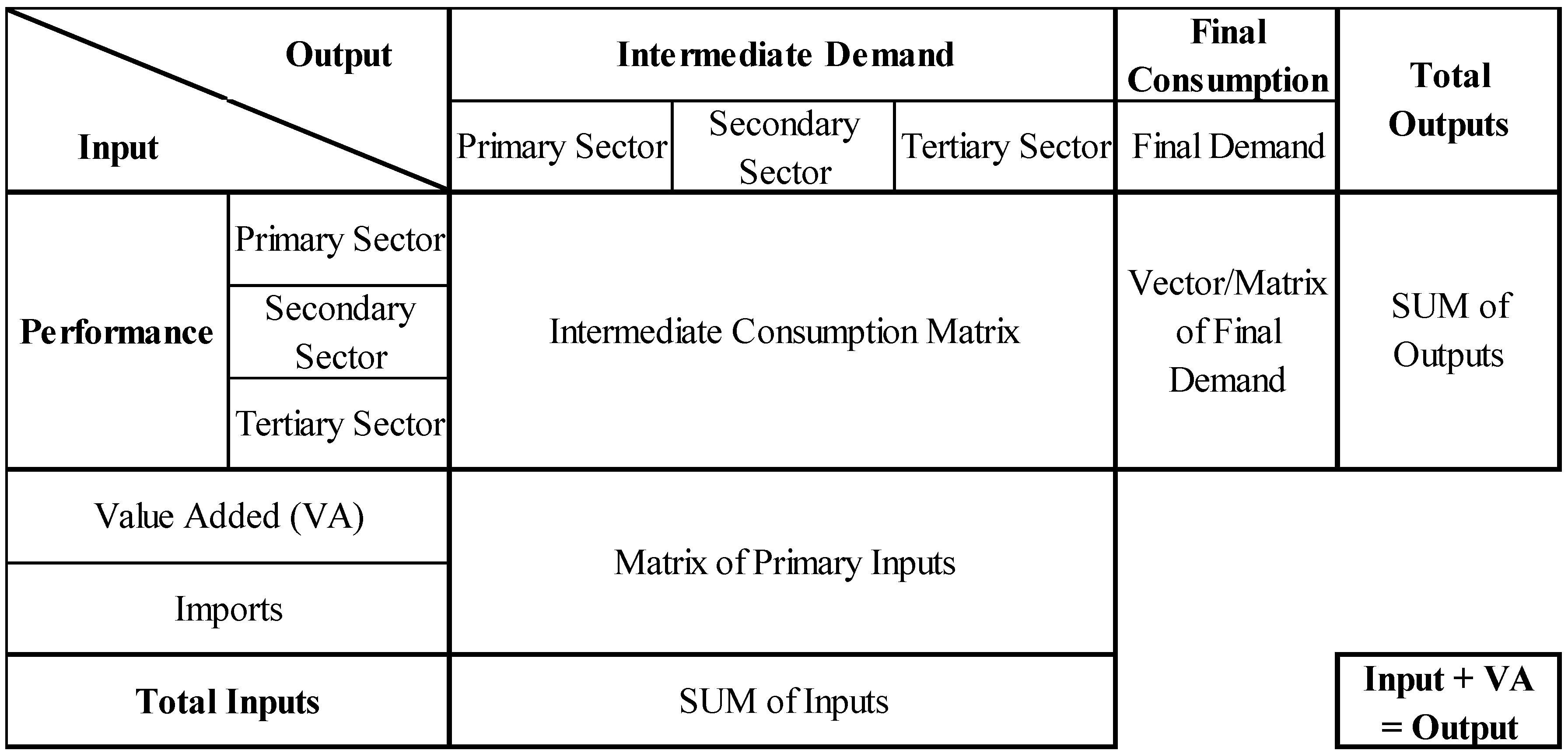
In a national economy, companies are often technologically and economically intertwined between several sectors. Thus, the value added by one company is usually part of a sector-overwhelming value chain, and, thereby, it depends on the value added by several other companies and sectors. The purpose of the input-output calculation is to mirror the linkages of production and goods in national economies in a matrix.

In this aforementioned matrix, the source and use of the economic sectors' inputs and outputs are given in monetary units. As DESTATIS [10] defines, inputs include both, intermediate consumption (supply with goods and services), and the production factors of labor and capital. The output of the economic sectors represents the value of the produced goods and services. A sector’s sum of total inputs and gross value added has to be equal to its total outputs. It is defined as the gross output value. Figure 1 represents this matrix schematically.

The input-output calculation is based on certain assumptions which lead to some limitations. The most important ones are briefly listed below:

• Time-based observation
  Input-output tables reflect only the status at a specific point in time. Accordingly, derived implications from these tables are only valid for the observed time and can be used for projections only to a limited extent.
• Homogeneity of goods
  Input-output calculations assume that each sector produces perfectly homogeneous goods. Therefore, aggregating several sectors leads to increasing uncertainties. According to Chakraborty and Raa [11], the often used and necessary aggregations of sectors lead to distortions in the input-output models. Consequently, to avoid distortions, input-output models should be calculated with tables that are aggregated as little as necessary.

For further readings on this topic, see the OECD [12].

2.3. Leontief Input-Output Model

The idea of today’s input-output calculation goes back to the economist Wassily Leontief [13], who received the Nobel economic prize for his input-output model, which is by far the most popular model. The Leontief model aims to explain the sectoral outputs (production of the sectors) due to respective final consumption of the end-user (final demand).

Let $X_i$ be the total output of sector $i$, $Z_{ij}$ the supply of sector $i$ for sector $j$ and $Y_i$ the final demand of products of sector $i$. The tabular correlations shown in Figure 1 can be mathematically formulated as follows:

$$X_i={{\displaystyle \sum }}_{j=1}^n{Z}_{ij}+Y_i$$

(1)

Let ${\alpha }_{\mathrm{L},ij}$ be the column-based standardization of $Z$ with its specific inputs $X_j$. The elements ${\alpha }_{\mathrm{L},ij}$ are, therefore, called input coefficients, see Erdmann and Zweifel [14]:

$${\alpha }_{\mathrm{L},ij}=\frac{Z_{ij}}{X_j}$$

(2)

The abovementioned Equation (1) can now be formulated with Equation (2) as the so-called Leontief production function Equation (3):

$$X_i={{\displaystyle \sum }}_{j=1}^n{\alpha }_{\mathrm{L},ij}·X_j+Y_i$$

(3)

Let $\overrightarrow{x_i}$ and $\overrightarrow{y_i}$ be the vectors which contain, respectively, the total outputs $X_i$ and the total final demands $Y_i$. Let ${\mathbf{A}}_{\mathbf{L}}$ be the matrix consisting of the standardized elements ${\alpha }_{\mathrm{L},ij}$. Using this, the abovementioned relation Equation (3) can be put in matrix notation Equation (4) and, by mathematical conversion, the outputs can be formulated in dependence on the final demand Equation (5),

$$\overrightarrow{x_i}={\mathbf{A}}_{\mathbf{L}}·\overrightarrow{x_i}+\overrightarrow{y_i}$$

(4)

$$\overrightarrow{x_i}=(\mathbf{I}-{\mathbf{A}}_{\mathbf{L}}{)}^{-1}·\overrightarrow{y_i}$$

(5)

The matrix $(\mathbf{I}-{\mathbf{A}}_{\mathbf{L}}{)}^{-1}$ with its elements ${\alpha }_{\mathrm{L},ij}$ is called Leontief inverse matrix. Assuming constant input coefficients, the elements of this matrix are also constant. In the Leontief model, the total sectoral outputs in equilibrium, therefore, depend only on the final consumption. The columns of the Leontief inverse matrix represent by how much the final demand in the particular sectors $j$ leads to demand in the upstream sectors $i$. Therefore, the Leontief model is often called the demand driven model, which is able to explain the backward linkages in economics.

According to Miller and Lahr [15], the rows of the Leontief inverse matrix were also used in former studies to study simplifying forward linkages. However, Steinback [16] argues that this approach is flawed and causes distortions because results obtained for the description of backward linkages are used to describe forward linkages.

The Leontief input-output model also has further limitations. Two of them are briefly explained below. For further detail, see the OECD [12].

• No possibilities for input substitution
  The outputs depend linearly on the inputs in the given ratios, due to the assumption of a fixed production function. Hence, intertwined sectors cannot create any output at all if one of the previous sectors has total failure.
• No scarcity of resources
  The Leontief input-output model assumes every raise in final demand can be satisfied by increasing the supply. Thus, the supply is only demand driven and is always able to cover the demand.

2.4. Ghosh Input-Output Model

In contrast to Leontief [13], Ghosh [17] introduced a model that uses an approach focusing on the columns instead of the rows of an input-output table. In this way, the sectoral inputs (demand of the sectors) are described by the primary inputs used. Since gross values added often have the largest share in the primary inputs, in literature often only gross values added are mentioned in this context.

Let $X_j$ be the total input of sector $j$, $Z_{ij}$ again the production of sector $i$ to sector $j$, and $V_j$ the primary inputs of sector $j$. The tabular correlations shown in Figure 1 can also be formulated mathematically as follows:

$$X_j={{\displaystyle \sum }}_{i=1}^n{Z}_{ij}+V_j$$

(6)

Let ${\alpha }_{\mathrm{G},ij}$ be the row-based standardization of $Z$ with its specific outputs $X_i$. The elements ${\alpha }_{\mathrm{G},ij}$ are, therefore, called allocation coefficients, see Park [18],

$${\alpha }_{\mathrm{G},ij}=\frac{Z_{ij}}{X_i}$$

(7)

Thereby, the abovementioned Equation (6) can be formulated with Equation (7) as follows:

$$X_j={\displaystyle \sum }_{i=1}^n{\alpha }_{\mathrm{G},ij}·X_i+V_j$$

(8)

Let $\overrightarrow{x_j}$ and $\overrightarrow{v_j}$ be the vectors which contain, respectively, the total inputs $X_j$ and the total primary inputs $V_j$. Let ${\mathbf{A}}_{\mathbf{G}}$ be the matrix consisting of the standardized elements ${\alpha }_{\mathrm{G},ij}$. Using this, the abovementioned relation can be put in matrix notation as well and by mathematical conversion, the inputs can be formulated in dependence on the final demand. Here, the superscript T expresses the transposition of a vector:

$${\overrightarrow{x_j}}^{\mathrm{T}}={\overrightarrow{x_j}}^{\mathrm{T}}·{\mathbf{A}}_{\mathbf{G}}+{\overrightarrow{v_j}}^{\mathrm{T}}$$

(9)

$${\overrightarrow{x_j}}^{\mathrm{T}}={\overrightarrow{v_j}}^{\mathrm{T}}·(\mathbf{I}-{\mathbf{A}}_{\mathbf{G}}{)}^{-1}$$

(10)

In analogy to the Leontief model, the matrix $(\mathbf{I}-{\mathbf{A}}_{\mathbf{G}}{)}^{-1}$ with its elements ${\alpha }_{\mathrm{G},ij}$ is called the Ghosh-inverse. Assuming constant allocation coefficients, the elements of this matrix are also constant. In this model, the sectoral total inputs in equilibrium depend only on the primary inputs used. The rows of the Ghosh inverse matrix represent by how much one unit of primary input in the sector $i$ leads to supply from this sector $i$ to its downstream sectors $j$. Therefore, the Ghosh model is often called supply-driven, which is able to explain forward linkages in economics.

However, the Ghosh input-output model has also certain limitations. Some of these limitations are briefly explained below.

• Perfect input substitutability
  Allocation coefficients are assumed to be constant in the Ghosh model. Hence, only the percentage distribution of a sector's output to downstream sectors is fixed. In contrast to the Leontief model, the percentage distribution of a sector’s inputs are variable, see Oosterhaven (1988).
• Scarcity of resources
  The Ghosh model assumes that a raise in production of one sector will automatically go along with increasing demand in the subsequent sectors. Thus, in this model, the demand is not a limiting factor in contrast to the supply. This is why the Ghosh model is often characterized as supply-driven.

Due to these limitations, the Ghosh model has been subject of controversial debates. In particular, the implication that the demand of downstream sectors reacts perfectly to changes in supply in upstream sectors has been criticized, see Oosterhaven [19], Oosterhaven [20] and de Mesnard [21]. Therefore, an increase of the supply would automatically lead to an increasing demand which is in fact a very implausible implication. Additionally, a reduction of a sector’s output of a given share would automatically lead to a reduction of the total gross value added of the economy with the same share.

However, there are counterarguments stating that these critics ignore the condition of inoperability of the suppliers under which Ghosh had formulated his model, see Park [18]. Following this idea and respecting the condition, the Ghosh model would be applicable to the special case of short-term output reductions (in contrast to increases or long-term structural changes), e.g., caused by natural disasters, terrorist attacks, etc.: demanders of a good are forced to react to short term reductions of supply quantities whereas they do not need to purchase larger quantities if supply is increased.

3. Underlying Data Basis

After having described the assumptions, we describe the necessary data for the modeling in this section. In particular, these are data from the monetary and energy based input-output tables, as well as the deflators of the gross domestic product.

3.1. Monetary Input-Output Tables

Since 1990, DESTATIS [10] has been publishing monetary input-output tables (MIOT) on a yearly basis in the context of the national income and product accounting for Germany, with a delay of multiple years each. These tables give information of the origin and usage of goods in 71 sectors. There are three different types of input-output tables published:

• Input-output tables of domestic production and imports
• Input-output tables of domestic production
• Import-matrices

In contrast to the input-output table of domestic production, the matrices that include imports do not integrate the imported goods for intermediate consumption in the intermediate consumption matrix. Instead, these imports are listed in the matrix of primary inputs and are not broken down to the specific sectors. Finally, the import-matrices show a detailed breakdown of sectoral origin and usage of the imported goods.

Currently, the latest input-output tables published by DESTATIS are those of 2010. However, the classification of economic sectors was changed after 2007. Thus, the input-output tables before and after 2007/2008 are not comparable. To get detailed description of the provided data for input-output tables of Germany, refer to DESTATIS [10].

3.2. Energetic Input-Output Tables

Besides monetary input-output tables (MIOT), which describe the economic and technologic interactions in monetary units, there are also physical input-output tables (PIOT), see DESTATIS [22]. In contrast to MIOTs, PIOTs measure the flows of goods not in monetary but in physical units. Since 1995, DESTATIS [23] publishes such PIOTs in the framework of environmental economic accounting. The PIOTs provide amongst others information about the origin and usage of energy, analyzed by energy sources and economic sectors, in the form of energetic input-output tables (short: EIOT). The contained data essentially consist of the data also used in energy balances, in Germany annually published by AG Energiebilanzen, plus data from additional sources. The energy use of 69 sectors is described in these tables.

From 1995 to 2005, the environmental economic accounting was published every five years. Since 2005, these statistics are published annually. Currently, the latest environmental economic accounting publication is from the reporting year 2012. The classification of economic sector in the energetic input-output tables was also changed between 2008 and 2009.

3.3. Deflators of Gross Domestic Product

In order to compare the monetary cash flows of different sectors for different years, they had to be adjusted for inflation. For this, the deflators in gross domestic product (GDP) for Germany, annually published by The World Bank [24], were chosen. The World Bank publishes the annual percentage change for each year.

The GDP-deflator can be defined as a measurement technique for inflation, which represents the ratio of the nominal GDP of a country to its real GDP. As it is distinct from other price indices like the consumer price index for Germany, the GDP-deflator is not based on a fixed basket with content that stays equal every year. Rather, the GDP-deflator rates all produced goods and services in the national economy in a specific year. Thus, the GDP-deflator is a broad-based price index that can be used to calculate price increases and inflation rates over the long-term.

Since this manuscript focuses on power interruption costs in economic sectors, we decided to use the GDP-deflator instead of the consumer price index. The usage of the consumer price index would be an inappropriate simplification because it only takes changes in prices of end products into account that are bought by average private households. However, sectors usually buy other products that are not bought by private households like raw metals or chemicals. The GDP-deflators for Germany have been adjusted to the chosen base year 2011.

4. Modeling

Following the microeconomic theory, profit maximization is the ultimate goal of companies through which their market behaviors can be explained, see Varian [25]. Companies combine multiple inputs in order to create value and generate profit. One of these inputs is usually electricity. If one of the production inputs is not accessible, the value adding process is often restricted or even impossible. In this section, we present two top-down models based on this idea that estimate the utility of electrical supply or, vice versa, the costs of power interruptions. The first model neglects that different economic sectors are usually linked to each other by supply and demand. The second model tries to take these inter-sectoral linkages into account.

4.1. Interruption Costs without Inter-Sectoral Linkages

In this model, unmade gross values added of the sectors are interpreted as their opportunity costs during a power outage. The sectoral gross values added have been published in monetary input-output tables for the specific years; see Section 3.1. We made the assumption of a linear correlation between power consumption and value added of a sector. The annual electricity consumptions of the specific sectors have been published in energetic input-output tables; see Section 3.2.

Under these conditions, the Value of Lost Load ${VOLL}_{i,\mathrm{I}}$ of a company in sector $i$ directly affected by an interruption is given by the division of the sector’s gross value added ${GVA}_i$ by its electricity consumption ${EC}_i$,

$${VOLL}_{i,\mathrm{I}}=\frac{{GVA}_i}{{EC}_i}$$

(11)

The sectoral classification of monetary and energetic input-output tables, however, differs partially because of the different systems used in certain years. The used classifications of the economic sectors were only based on the same classification system for the reporting years 2000, 2005, 2006, and 2007. Thus, this analysis was only feasible with data from these particular years. In spite of the same classification system used for these reporting years, the sectoral classifications in both input-output tables differ regarding the level of detail. For this reason, we chose to aggregate the sectoral classifications anew in such a way where the sectors in these two tables (MIOT and EIOT) overlap with the highest possible level of detail. In the end, this gives us a classification of the economy in 51 sectors, which is quasi the lowest common denominator.

After the analysis, the 51 sectors were aggregated again, in 12 and finally three sectors for better clarity and presentability. For this, we use the same classification and aggregation method as the one used by DESTATIS. The classification in 12 sectors can be further aggregated into the three sector classification:

• Sector 1 corresponds to the primary sector (agriculture)
• Sectors 2 to 8 correspond to the secondary sector (industry)
• Sectors 9 to 12 correspond to the tertiary sector (services)

Furthermore, to ensure comparability of the results in the different reporting periods, all monetary quantities were adjusted to the base year 2011 by using the deflators presented in Section 3.3.

4.2. Interruption Costs with Sectoral Linkages

As already described in the previous sections, different sectors in a value chain are often economically and technologically intertwined. Production losses in a sector $i$ due to power interruptions can therefore cause production losses in subsequent sectors $j$. For this reason, the ${VOLL}_{i,\mathrm{II}}$ was introduced in addition to the ${VOLL}_{i,\mathrm{I}}$. The Roman numeral II stands for the second model. The ${VOLL}_{i,\mathrm{II}}$ includes not only the ${VOLL}_{i,\mathrm{I}}$ but also consequential opportunity costs in the downstream sectors $j$ that are caused by power interruptions in sector $i$. Thus, inter-sectoral forward linkages need to be quantified. In order to do so, we decided to employ a methodology which is based on the supply driven Ghosh model.

To determine the ${VOLL}_{i,\mathrm{II}}$, the same database which was used for the ${VOLL}_{i,\mathrm{I}}$ was applied: monetary input-output tables adjusted for inflation, and energetic input-output tables for the reporting years 2000, 2005, 2006, and 2007. Furthermore, the economic sectors were also classified in 51 sectors and the results were summarized in 12 and three sectors.

The algorithm to determine the ${VOLL}_{i,\mathrm{II}}$ is explained in detail in the following.

4.2.1. Effects of Output Reductions in Sector i on the Output in Sector j

First, we calculated the Ghosh inverse matrices for the monetary input-output tables of the chosen reporting years. With this as a basis, a Ghosh model was built. The Ghosh model describes the production depending on the primary input. However, the final aim in the present case is to quantify the effect of decreased production in a sector $i$ to downstream sectors $j$. Thus, we need to apply certain modifications to the Ghosh model.

Steinback [16] presents an algorithm for this purpose which is appropriate for an application with a backward-linked Leontief model. In this algorithm, the Leontief inverse matrix is modified in a way where the output of sector $j$ can be described by the change of the output in sector $i$. For that, the elements ${\alpha }_{\mathrm{L},ij}$ of the Leontief inverse matrix are divided column-wise with the diagonal entries ${\alpha }_{\mathrm{L},jj}$.

In analogy to Steinback’s approach, we carried out the following modification for the Ghosh model:

• $\Delta v_i$ be the change of the primary input in sector $i$,
• ${\alpha }_{\mathrm{G},ij}$ be the element in row $i$ and column $j$ of the Ghosh inverse matrix, and
• $\Delta x_j$ be the change in the gross output value of sector $j$.

Assuming the other sectors’ primary inputs to stay constant, we find the following Equation (12).

$$\Delta x_j=\Delta v_i·{\alpha }_{\mathrm{G},ij}$$

(12)

Resulting from this, we can derive the following Equation (13) for sector $i$ itself from Equation (12),

∆x_i = ∆v_i ∙ α_G,ii

(13)

The substitution of $\Delta v_i$ in Equation (12) with $\Delta v_i$ from Equation (13) leads to the following Equation (14), which represents $\Delta x_j$ (the change in the gross output value of sector $j$) depending on $\Delta x_i$ (the change in the gross output value of sector $i$).

$$\Delta x_j=\Delta x_i·\frac{{\alpha }_{\mathrm{G},ij}}{{\alpha }_{\mathrm{G},ii}}$$

(14)

Thus, the elements of the Ghosh inverse matrix are row-serially divided by the corresponding diagonal element in the inverse matrix.

4.2.2. Effects of Gross Value Added Reductions in Sector i on the Gross Value Added in Sector j

Furthermore, we needed to quantify the effects of changes in ${GVA}_i$ (gross value added of sector $i$) on ${GVA}_j$ (gross value added of sector $j$). In order to formulate such a multiplier $f_{ij},$ we still had to adjust ${\alpha }_{\mathrm{G},ij}/{\alpha }_{\mathrm{G},ii}$ (elements of the modified Ghosh inverse).

Since the sum of the outputs is equal to the gross production value $GPV$, the elements ${\alpha }_{\mathrm{G},ij}/{\alpha }_{\mathrm{G},ii}$ were multiplied by the ratio of the gross production value to the gross value added of sector $i$, ${GPV}_i/GV{A}_i$, and by the ratio of the gross value added to the gross production value of sector $j$, $GV{A}_j/GP{V}_j$. Therefore, we obtain the multiplier $f_{ij}$ through Equation (15),

$$f_{ij}=\frac{GP{V}_i}{GV{A}_i}·\frac{{\alpha }_{\mathrm{G},ij}}{{\alpha }_{\mathrm{G},ii}}·\frac{{GVA}_j}{{GPV}_j}$$

(15)

4.2.3. Effects of Gross Value Added Reductions in Sector i on the Gross Values Added of All Following Sectors j

We then calculated the multiplier $f_i$ which indicates by how much the total value added in the national economy decreases, if the value added in sector $i$ is decreased by one monetary unit. For this, the row-sums of the matrix with its elements $f_{ij}$ have been computed,

$$f_i={\displaystyle \sum }_{j=1}^n{f}_{ij}$$

(16)

4.2.4. Calculation of the Values of Lost Load (VOLL) II Based on the VOLL I

Finally, we calculated the ${VOLL}_{i,\mathrm{II}}$ by multiplying the ${VOLL}_{i,\mathrm{I}}$ with the estimated multiplier $f_i$, see Equation (17),

$${VOLL}_{i,\mathrm{II}}={VOLL}_{i,\mathrm{I}}·f_i$$

(17)

5. Results

The results for the three sector classifications are shown in

Table 1. Results for the VOLL (Values of Lost Load) I in a three sector division in EUR/kWh.

Sector	VOLL I in EUR/kWh
	2000	2005	2006	2007
Primary sector	4.62	3.07	3.11	3.53
Secondary sector	1.94	1.83	1.93	1.96
Tertiary sector	12.29	12.88	12.75	13.23

(VOLL I, without linkage effects) and

Table 2. Results for the VOLL II in 3 sectors in EUR/kWh.

Sector	VOLL II in EUR/kWh
	2000	2005	2006	2007
Primary sector	6.97	4.85	4.93	5.46
Secondary sector	3.91	3.16	3.25	3.33
Tertiary sector	16.77	16.94	16.59	17.32

(VOLL II, with linkage effects).

Table 3. Results for the VOLL I in a 12 sector division.

Sector	VOLL I in EUR/kWh
	2000	2005	2006	2007
Agriculture and forestry	4.62	3.07	3.11	3.53
Mining, energy and water	0.67	0.72	0.78	0.83
Chemical and petroleum products	0.87	0.89	0.94	0.89
Metalworking	1.17	1.11	1.21	1.26
Machinery, vehicles, electronics	4.87	4.90	5.21	5.13
Textiles, wood, paper	1.81	1.52	1.51	1.56
Food and beverages	2.13	1.83	1.79	1.79
Construction work	29.86	24.16	22.92	23.94
Commerce, traffic, communication, restaurants	5.64	5.62	5.66	5.83
Banks, insurances, housing industry	39.59	38.39	39.57	41.22
Healthcare and social work services	15.47	17.06	15.53	16.00
Public administration, culture, private household services	12.55	13.17	12.81	13.57

(VOLL I, without linkage effects) and

Table 4. Results for the VOLL II in a 12 sector division.

Sector	VOLL II in EUR/kWh
	2000	2005	2006	2007
Agriculture and forestry	6.97	4.85	4.93	5.46
Mining, energy and water	2.35	1.68	1.68	1.78
Chemical and petroleum products	1.65	1.55	1.63	1.61
Metalworking	2.06	1.88	2.07	2.16
Machinery, vehicles, electronics	5.86	5.82	6.12	6.05
Textiles, wood, paper	2.77	2.39	2.33	2.41
Food and beverages	2.76	2.37	2.28	2.31
Construction work	41.81	33.50	31.89	33.53
Commerce, traffic, communication, restaurants	8.15	7.62	7.60	7.91
Banks, insurances, housing industry	59.84	56.47	57.42	59.44
Healthcare and social work services	16.38	18.20	16.51	17.07
Public administration, culture, private household services	14.97	16.04	15.63	16.59

(VOLL I, without linkage effects) and Table 2 (VOLL II, with linkage effects) show the results for the 12 sector classification.

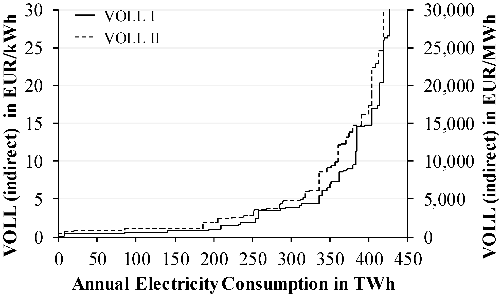
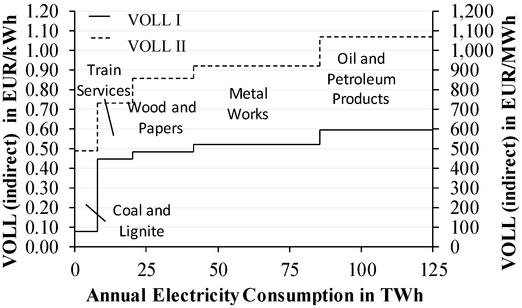
For reasons of clarity, the results for the 51 sector classification are graphically illustrated in Figure 2 as boxplots and in Figure 3 and Figure 4 in weighted and ordered graph bars as the mean averages over the four years. The ordinate in Figure 3 has been cut off at 30 EUR/kWh for reasons of visualization. Figure 4 represents a detail of Figure 3 with the lowest VOLL for the first 125 TWh of power consumption. The detailed results are shown in

Table A1. Results for the VOLL I in a 51 sector division.

Sector	VOLL I in EUR/kWh
	2000	2005	2006	2007
Agriculture, hunting, and forestry	4.72	3.28	3.34	3.83
Fishing	1.55	1.72	1.70	2.16
Coal and lignite	0.03	0.08	0.09	0.12
Crude oil and natural gas	3.34	2.31	4.54	3.90
Ore mining and quarrying	–	–	–	–
Stone and earth mining and quarrying	1.63	1.50	1.69	1.75
Food products and beverages	2.07	1.90	1.86	1.89
Tobacco	4.59	3.42	4.04	3.64
Textiles	1.21	1.63	1.62	1.72
Clothing	3.02	8.55	9.45	14.51
Leather	2.31	4.63	4.28	5.59
Wood and products of wood and cork	1.76	1.48	1.48	1.47
Pulp, paper, and paper products	0.51	0.46	0.48	0.47
Printing and publishing	6.59	4.81	4.23	6.23
Coke, refined petroleum products and nuclear fuel	0.51	0.71	0.84	0.59
Chemicals and chemical products	0.70	0.80	0.86	0.87
Rubber and plastics products	1.58	1.59	1.55	1.52
Other non-metallic mineral products	1.05	0.94	0.97	0.92
Basic metals	0.44	0.49	0.53	0.62
Fabricated metal products	4.17	3.75	3.96	3.81
Machinery and equipment	6.75	7.27	7.48	7.85
Computer, Electronic and optical equipment	11.77	11.87	9.49	12.28
Electrical machinery and apparatus	6.41	5.97	6.57	5.69
Communications equipment and facilities	4.22	3.50	3.23	4.33
Medical, measurement, control, optical instruments	8.68	10.22	10.17	7.00
Motor vehicles, trailers and semi-trailers	2.86	3.45	3.89	3.97
Other transport equipment	3.02	3.90	4.24	4.26
Furniture, other manufactured goods	4.03	4.32	3.95	4.16
Secondary raw materials	1.45	1.48	1.66	2.16
Electricity and district heating	0.53	0.59	0.61	0.64
Manufactured gas, distribution services of gases	3.86	6.23	7.73	10.41
Water and distribution services of water	1.93	2.63	2.56	2.85
Construction	29.86	25.47	24.25	25.74
Wholesale and retail trade and repair of motor vehicles	6.99	9.86	10.28	10.67
Wholesale trade and commission trade	19.83	16.12	14.57	17.38
Retail trade services	4.29	4.25	4.51	4.61
Restaurants and hotels	3.46	3.50	3.30	3.73
Rail services	0.38	0.44	0.47	0.49
Other land transport, transport via pipelines	5.99	6.26	6.65	6.89
Water transport services	–	–	–	–
Air transport services	11,072.95	10,753.74	2037.81	2250.57
Supporting and auxiliary transport services	6.78	8.96	9.28	9.74
Message transmitting services	8.12	9.32	9.46	7.54
Credit and insurance trade	19.60	28.15	29.56	28.68
Services (real estate, databases, R & D, business services)	47.45	43.84	44.89	48.01
Public administration, defence, obligatory services	12.49	15.46	15.07	15.96
Education	17.94	21.95	20.03	21.46
Health care sector	13.68	15.71	14.34	14.84
Waste water, waste disposal	24.76	26.61	25.84	26.57
Culture, sport, and entertainment services	10.01	8.59	8.42	8.89
Activities of membership organizations, other services	15.81	17.40	16.83	19.55

and

Table A2. Results for the VOLL II in a 51 sector division.

Sector	VOLL II in EUR/kWh
	2000	2005	2006	2007
Agriculture, hunting, and forestry	7.15	5.21	5.33	5.95
Fishing	1.93	2.06	2.00	2.60
Coal and lignite	0.44	0.45	0.44	0.63
Crude oil and natural gas	4.00	2.82	5.38	4.93
Ore mining and quarrying	–	–	–	–
Stone and earth mining and quarrying	3.42	3.34	3.54	3.56
Food products and beverages	2.70	2.47	2.37	2.46
Tobacco	4.59	3.42	4.04	3.64
Textiles	1.48	2.03	1.97	2.08
Clothing	3.15	8.96	10.05	15.36
Leather	2.77	5.40	4.94	6.47
Wood and products of wood and cork	3.27	2.74	2.78	2.78
Pulp, paper, and paper products	0.94	0.82	0.84	0.82
Printing and publishing	11.53	8.22	7.31	10.70
Coke, refined petroleum products and nuclear fuel	2.23	2.84	3.52	2.98
Chemicals and chemical products	1.09	1.13	1.19	1.19
Rubber and plastics products	2.68	2.56	2.52	2.53
Other non-metallic mineral products	2.05	1.82	1.85	1.75
Basic metals	0.79	0.86	0.93	1.08
Fabricated metal products	6.58	5.86	6.14	6.08
Machinery and equipment	7.99	8.49	8.68	9.12
Computer, Electronic and optical equipment	20.90	19.83	15.33	19.04
Electrical machinery and apparatus	9.48	8.99	9.60	8.41
Communications equipment and facilities	5.70	4.79	4.33	5.67
Medical, measurement, control, optical instruments	10.10	11.01	11.09	7.66
Motor vehicles, trailers and semi-trailers	3.08	3.68	4.13	4.22
Other transport equipment	3.72	4.98	5.28	5.46
Furniture, other manufactured goods	4.34	4.67	4.28	4.53
Secondary raw materials	3.86	4.42	4.66	5.53
Electricity and district heating	0.99	1.07	1.07	1.14
Manufactured gas, distribution services of gases	6.82	11.01	13.39	17.79
Water and distribution services of water	2.72	3.89	3.79	4.24
Construction	41.81	35.33	33.73	36.05
Wholesale and retail trade and repair of motor vehicles	9.12	12.57	13.09	13.89
Wholesale trade and commission trade	29.63	23.26	20.98	24.63
Retail trade services	4.59	4.56	4.88	4.99
Restaurants and hotels	3.93	3.59	3.32	3.74
Rail services	0.72	0.69	0.72	0.79
Other land transport, transport via pipelines	12.10	12.92	13.67	14.19
Water transport services	–	–	–	–
Air transport services	21,069.70	23,777.20	4588.26	5198.31
Supporting and auxiliary transport services	15.01	17.82	18.10	18.78
Message transmitting services	14.12	14.81	14.76	11.79
Credit and insurance trade	34.26	48.33	49.46	47.39
Services (real estate, databases, R & D, business services)	67.32	61.55	62.68	66.84
Public administration, defence, obligatory services	13.62	16.98	16.51	17.54
Education	19.47	24.33	21.92	23.73
Health care sector	13.77	15.80	14.45	14.93
Waste water, waste disposal	43.28	48.07	47.54	49.65
Culture, sport, and entertainment services	13.65	11.72	11.55	12.27
Activities of membership organizations, other services	20.61	22.87	22.27	25.79

in the Appendix of the manuscript.

6. Discussion

The methodology presented in this manuscript allows on the one hand a quantitative overview of the distribution of Values of Lost Load (VOLL) across the economy over a large number of very heterogeneous sectors. On the other hand, the methodology allows a quantification of inter-linkage effects across different sectors and the economy which are triggered by power interruptions occurring in single sectors. However, even though the focus of the present manuscript is a different one, we want to point out that there exist other important factors to the cost of power interruptions besides the heterogeneity of different sectors and inter-linkage effects such as the duration and frequency or the moment in time (day, week, season, etc.) of interruptions. However, as representative data for all of the 51 economic sectors is scarce, we eventually decided to not include more factors influencing the VOLL (e.g., there are no known publications of representative data of load profiles for all of the 51 economic sectors). We therefore recommend a more in-depth analysis of a few selected sectors that show the largest potentials. For the application of methodologies that include an estimation of some of these previously named effects, please refer to Growitsch et al. [6] or Reichl et al. [26].

The results support our first initial hypothesis (see Section 1). We can indeed observe a very strong heterogeneity of interruption cost in the results among different economic sector with the VOLLs being distributed very unequally over all examined economic sectors. Still, certain trends can be observed and are briefly explained in the following. The results indicate that manufacturing companies (from the secondary sector) generally tend to have the lowest VOLL. The mean average in this sector is 1.91 EUR/kWh (VOLL I) and increases under consideration of interlinkage-effects with a multiplier of around 1.8 to up to 3.41 EUR/kWh (VOLL II). The results for the division in 51 sectors show that companies of the construction industry are outliers with a high VOLL I of 26.33 EUR/kWh and a VOLL II of 36.73 EUR/kWh. A possible explanation for this is that the measurement of power consumption is difficult at building sites and might be underestimated. Schlomann et al. [27] suggest that the reason for this problem is that the costs for electricity are usually borne by the owner and not by the building contractor. In the height of the VOLL, the manufacturing companies (from the secondary sector) are followed by the companies of agriculture (from the primary sector). For the agriculture companies, the average VOLL I is 3.58 EUR/kWh and increases in the case of VOLL II with a multiplier of 1.6 to up to 5.55 EUR/kWh. The highest VOLL comes by far from general service-providing companies of the tertiary sector. The average VOLL I in this sector equals 12.79 EUR/kWh. The average VOLL II is 16.91 EUR/kWh, so that the multiplier between both VOLLs is around 1.3. In the 12-sectoral classification, the financial services sector (banks, insurances, housing industry) is the economic sector with the highest VOLL. This sector’s VOLL I is 36.69 EUR/kWh and increases with a multiplier of 1.6 to 58.29 EUR/kWh (VOLL II). An explanation for the observed heterogeneity is the fact that VOLL is in our case dependent on the energy consumption. Sectors with relatively high energy consumption (industry) have a rather low VOLL and vice versa (services).

Nevertheless, sectors with extremely high VOLL and sectors with very low VOLL might turn out to be interesting candidates for certain fields of application indicating an important added value of such analyses over analyses of average figures. The cases of emergency power supply and load shedding actions shall be used as examples in the further discussion. Relatively high VOLL of a specific sector indicate that electricity is a rather critical input of a sector. A power interruption would be accompanied by high costs compared to expenditures with the originally planned power consumption. Therefore, high VOLL might be a good indicator that the specific sectors should be equipped with emergency backup systems due to potentially very high interruption costs. From an economical point of view, this is a convenient measure if the average costs of electricity generation of those emergency power supply systems are lower or equal to the VOLL. Sectors with lowest VOLL might be potential candidates for load shedding measures from the perspective of the entire energy system. Such measures might be economically optimal if other possibilities of providing short-term needed electricity (e.g., backup or storage capacities) are more expensive than the VOLL of the candidate. Under circumstances, load shedding may even prevent extensive blackouts for all electricity consumers, including consumers with high VOLL. We want to point out that there exist other forms of demand response besides load shedding that are less severe such as load shifting, see see Grein and Pehnt [28].

However, in this method, direct cost elements, for example caused by damage of production facilities or electronic devices, are not determined. This is very common for macroeconomic studies, see Sullivan and Keane [1]. But in the end, the actual occurring costs might be higher. This hints to the following new hypothesis:

The actual costs approach the costs that were determined here, if the affected companies can prepare for a planned power interruption with a sufficient lead time. The direct costs can most likely be minimized by an early enough announcement of the power interruption. 

Furthermore, the results also support our second (and last) initial hypothesis (see Section 1). If economical linkages are also considered, a very significant increase in costs can be observed in the results. The standardized Ghosh-multiplier between VOLL I and VOLL II has its power consumption weighted average at around 1.7. Sectors producing goods used towards the beginning of value chains have a higher standardized Ghosh-multiplier compared to sectors producing goods used towards the end of value chains. For example, the standardized Ghosh-multiplier in the sector of coal and peat is about 7.4 in average, which is relatively high. Interestingly enough, this multiplier trend declines over time. In the year 2000, this multiplier is 13.4. In the years 2005 to 2007, this multiplier shows up in the range of only 4.9 to 5.8, which is still a high multiplier in comparison. For example, the standardized Ghosh-multiplier in the sectors of tobacco products or of restaurant services comes to relative low values of averagely 1.0.

For this reason, the question comes up in which cases the VOLL I and in which cases the VOLL II are appropriate to determine the economic consequences of a power interruption. These insights lead to the formulation of a new hypothesis:

Production interruptions might be compensated with stocks and warehousing. If interruptions are sufficiently short, the average costs tend to be limited to the VOLL I. Since, however, the capacity of those stocks is finite, existing buffer possibilities might be too small for long-term interruptions. In such cases, the economic costs stretch to ongoing sectors so that the VOLL II becomes relevant. 

7. Conclusions

The increasing share of intermittent power generation poses high challenges for the supply security. The increase will make it more and more difficult (and with that more costly) to maintain the currently very high level of supply security. If the cost to maintain and increase supply security remain constant, this means that the welfare optimal level of supply security decreases. The present work seeks to make a scientific contribution to the question of what the value of reliable power supply is by quantifying the consequences of power interruptions monetarily as an overview of non-household power consumers. On the one hand, our focus lies in reflecting the heterogeneity of the results for different consumer groups by dividing non-household consumption into a relatively large number of 51 economic sectors. On the other hand, the goal was to quantify inter-linkage effects between different sectors.

The results support the general assumption that power interruptions lead, in average, to high cost for economic sectors, and that supply security has a rather high utility level for them. We estimated power interruption cost for directly affected economic sectors as Value of Lost Load I (VOLL I) and power interruption cost taking effects in downstream sectors through inter-sectoral linkages into account as the Value of Lost Load II (VOLL II).

However, a detailed analysis of the VOLL between different sectors reveals that the frequency distribution of these costs is widely spread. Some sectors have rather low interruption costs, whereas other sectors have very high interruption costs (heterogeneity). Load shedding measures, meaning selective (voluntary) interruptions of costumers with the lowest Value of Lost Load, could prove to be more cost-efficient than the construction and operation of storage or generation capacities for only a few hours in a year. According to the results, companies of the sectors coal and lignite, railway services, wood and paper and metals might be interesting candidates for these measures with a Value of Lost Load of approximately 0.50 EUR/kWh. The levelized cost of electricity (LCOE) of a peak load gas turbine with 100 full load hours per year should be around that cost figure of 0.50 EUR/kWh.

As already discussed, there are other very important factors influencing the cost of power interruptions besides those that we analyze in this manuscript such as duration or frequency of an interruption, time of an interruption (hour, weekday, season, public holiday, etc.), the availability of backup batteries, etc. The results presented here can be seen as a starting point to identify sectors with potential for demand-side management or even load shedding and to understand their inter-linkage with other sectors. We suggest that future studies should apply other methods for estimating VOLL (such as micro-economic approach or methods of revealed or stated preferences) for the selected sectors with economic potential in order to refine results for only a small limited number of sectors with regard to the aforementioned influencing factors. Furthermore, the results provided in this manuscript can only be seen as a first indication and overview of the cost of less severe demand response measures in the sectors. Applying less severe demand response measures might lower the cost and increase the economic potential. Therefore, more detailed research of a selected few sectors is recommended.