Article

Power Quality Disturbances Feature Selection and Recognition Using Optimal Multi-Resolution Fast S-Transform and CART Algorithm

School of Electrical Engineering, Northeast Electric Power University, Jilin 132012, China
*
Author to whom correspondence should be addressed.
Energies 2016, 9(11), 927; https://doi.org/10.3390/en9110927
Submission received: 24 August 2016 / Revised: 26 October 2016 / Accepted: 2 November 2016 / Published: 9 November 2016
(This article belongs to the Special Issue Microgrids 2016)

Abstract

:
In order to improve the recognition accuracy and efficiency of power quality disturbances (PQD) in microgrids, a novel PQD feature selection and recognition method based on optimal multi-resolution fast S-transform (OMFST) and classification and regression tree (CART) algorithm is proposed. Firstly, OMFST is carried out according to the frequency domain characteristic of disturbance signal, and 67 features are extracted by time-frequency analysis to construct the original feature set. Subsequently, the optimal feature subset is determined by Gini importance and sorted according to an embedded feature selection method based on the Gini index. Finally, one standard error rule subtree evaluation methods were applied for cost complexity pruning. After pruning, the optimal decision tree (ODT) is obtained for PQD classification. The experiments show that the new method can effectively improve the classification efficiency and accuracy with feature selection step. Simultaneously, the ODT can be constructed automatically according to the ability of feature classification. In different noise environments, the classification accuracy of the new method is higher than the method based on probabilistic neural network, extreme learning machine, and support vector machine.

1. Introduction

A microgrid can not only achieve grid-connected operation with distributed generators and a flexible and effective access distribution network, but also can run on islands. To some degree, this improves the reliability of the power supply and power quality (PQ) of the grid. However, the intermittent and random output characteristics of the distributed generators, such as photovoltaic and wind power, directly affect the microgrid’s voltage quality. Meanwhile, in order to realize distributed power consumption and flexible scheduling, a lot of nonlinear power electronic equipment is widely used and system operations (power and compensation capacitor switching) are frequently carried out in the microgrid. As a result, these lead to an increase in the number of PQ disturbance events [1,2,3,4]. In addition, the transient faults (including ground faults and phase faults, etc.) can lead to the breakdown of line insulation, power outages, and other serious consequences. Therefore, the PQ in the microgrid is further deteriorated [5,6,7,8].
Accurate recognition of power quality disturbances (PQD) is an important prerequisite and foundation for improving the PQ of the microgrid [9]. In the smart microgrid, it is necessary to carry out PQ monitoring for microgrid networks and distributed generators. In this process, a large amount of PQ data has been accumulated, which has put forward higher efficiency requirements for PQD analysis methods [10]. On the other hand, due to short duration and small changes in the electrical indicators, PQD analysis is more difficult [11,12]. Furthermore, compared to the PQ monitoring and analysis for traditional transmission network, the PQ signals recorded in the microgrid have many more noise components. The amplitude and frequency of the voltage change are irregular and the range of fluctuation is larger, which further increases the difficulty of PQD analysis [13]. Consequently, we should design an efficient classifier with high accuracy and noise immunity to improve the ability and efficiency of PQD recognition in microgrid.
Features extracted from the time-frequency analysis method are always used as the input of the classifier for PQD recognition. Common signal processing approaches used for PQD signal processing include fast Fourier transform (FFT) [14], wavelet transform (WT) [15,16], Hilbert-Huang transform (HHT) [17], and S-transform (ST) [18,19,20,21,22,23]. Of the existing methods, ST and its modified forms are widely used for feature extraction of disturbance signals and have achieved good effects [18,19,20,21,22,
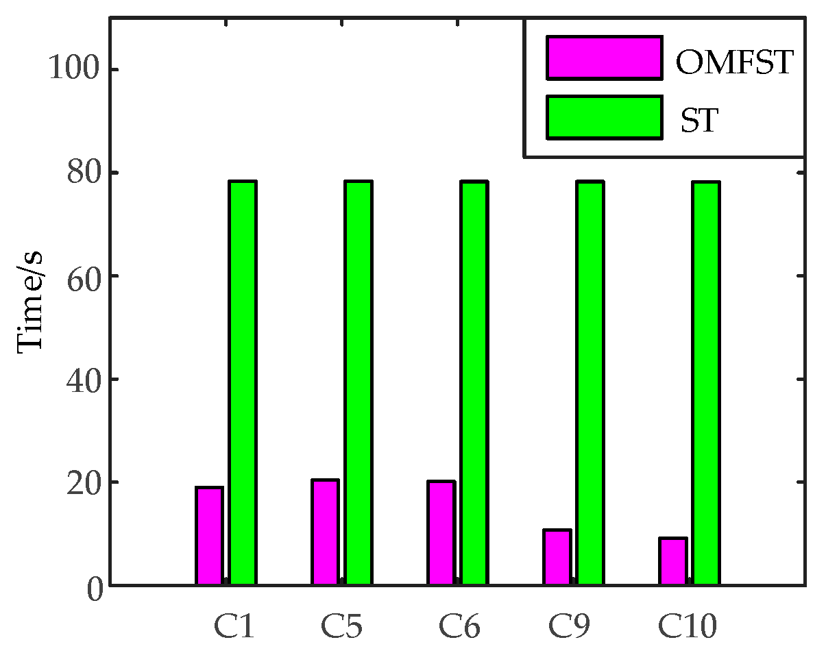
23]. ST has powerful time-frequency analysis ability and is not sensitive to noise, which is conducive to the extraction of multiple time-frequency features for PQD recognition. However, the major limitation of ST is its high computational and spatial complexity.
Feature extraction of disturbance signals is generally carried out in specific parts of the ST modulus matrix. Thus, we need not carry out inverse fast Fourier transform (IFFT) on the entire frequency area. Some researchers have proposed a fast S-transform (FST) method. Compared to ST, FST selects the main disturbance frequency points and only carries out IFFT on the selected frequencies to minimize the number of computations [19,20]. However, the frequency domain energy of transient oscillation is widely distributed in the high frequency range with short duration and small energy. The main disturbance frequency domain is difficult to get through the FFT spectrum, especially in high noise environments. Hence, the existing FST methods cannot completely satisfy the needs of disturbance recognition. In addition, when disposing complex disturbances, the time resolution and frequency resolution of ST and FST, which are conditioned by the Heisenberg uncertainty principle, cannot be satisfied simultaneously with a uniform time-frequency window width factor. As for the analysis of the complex disturbance with harmonic and sag component, the harmonic component analysis requires a higher frequency resolution, while sag component analysis requires a higher time resolution. Accordingly, multi-resolution generalized S-transform (MGST) [21] is designed with different window width factors in different frequency ranges to enhance the performance for complex PQD signals analysis. Although the demand of feature extraction of complex disturbance signals is satisfied, the redundant computation is still in existence.
In the pattern recognition of PQD, probabilistic neural network (PNN) [24,25], extreme learning machine (ELM) [26], support vector machine (SVM) [27,28,29], and decision tree (DT) [19,30,31,32,33] have been applied for PQD recognition and achieved good classification results. Compared with other classifiers, the DT has a simple structure, high classification efficiency, and accuracy. It is suitable for real applications with high real-time requirements. Meanwhile, it is convenient to achieve in a low-cost embedded system, and can satisfy the demands of efficiency, accuracy, and cost of PQ big data analysis [19,30,31,32,33]. However, the effects of DT depend on the determination of feature selection and classification threshold. For one thing, the existing DT classifiers are used to determine the features and classification thresholds based on statistical experiments, which makes it easier to fall into overfitting. Moreover, the DT methods used in the PQD analysis area are not optimal or automatic. All of these limitations affect the classification performance of DT classifier. For another, due to the interference of noise signals, the optimal threshold of each node of DT is changed greatly. So, it is difficult to design a DT classification system that can meet the classification accuracy requirements under different levels of noise.
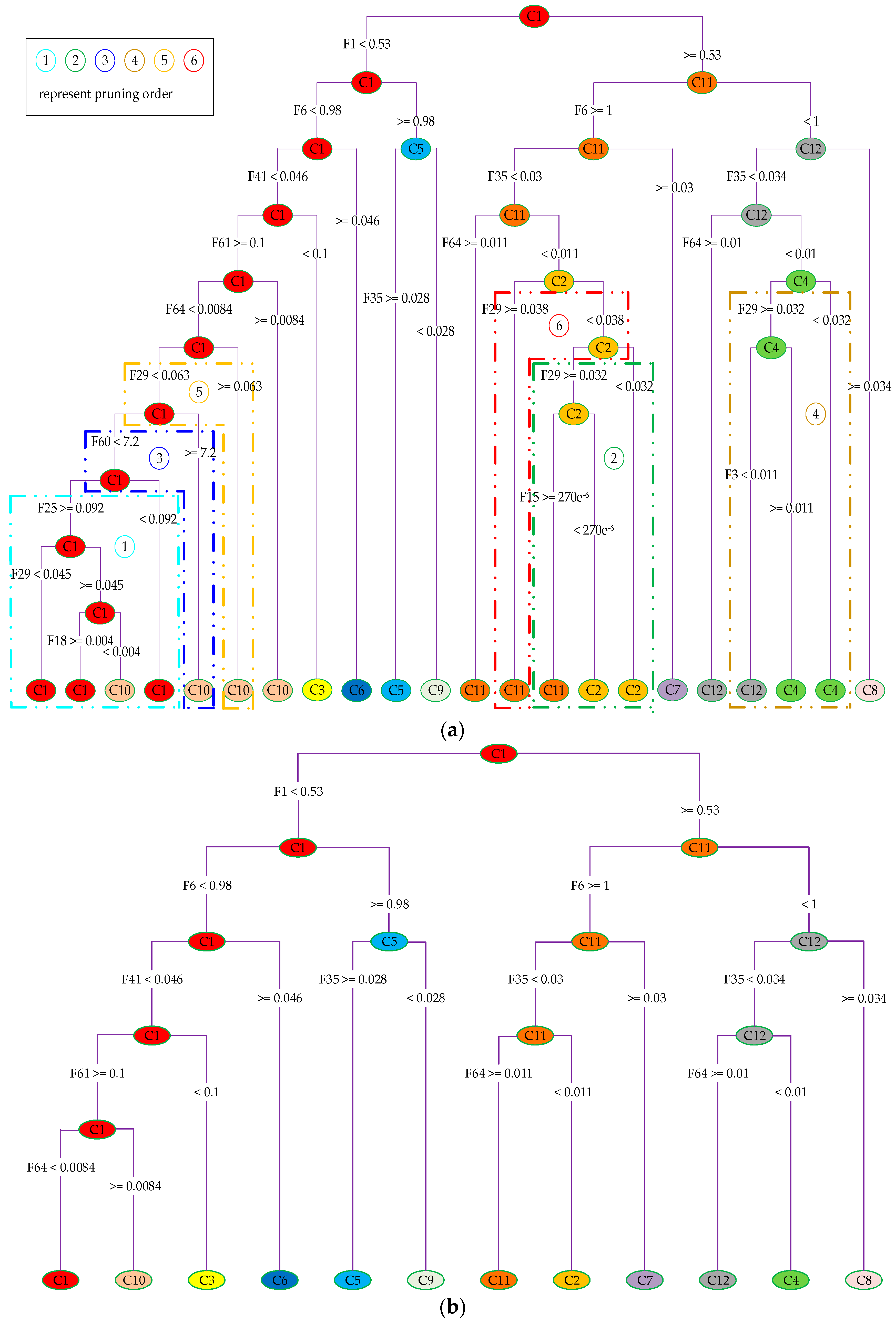
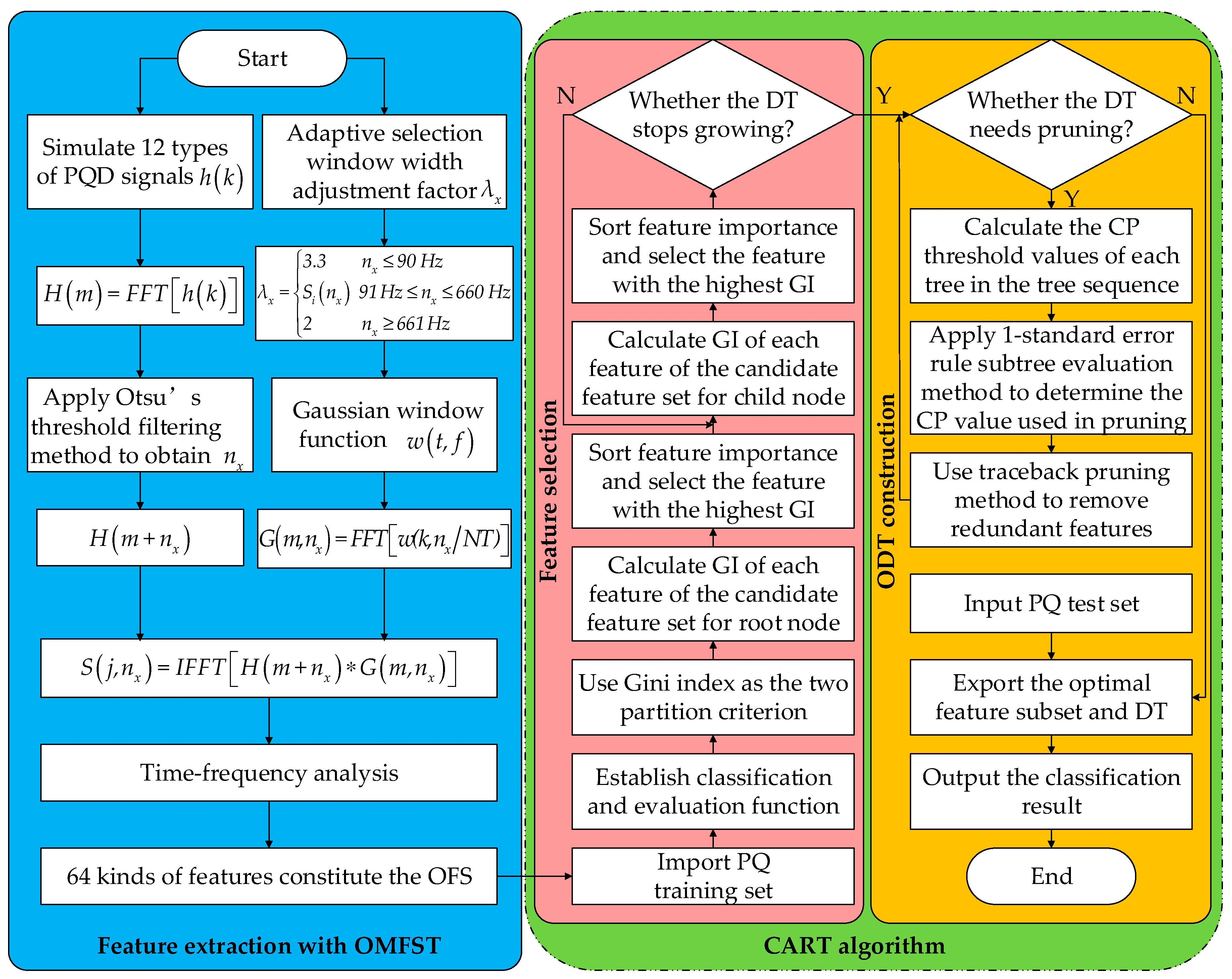
In order to solve the limitations, a novel PQD feature selection and optimal decision tree (ODT) construction method using optimal multi-resolution fast S-transform (OMFST) and classification and regression tree (CART) algorithm is proposed in this paper. Firstly 12 kinds of PQD signals including six kinds of complex disturbances are simulated by a mathematical model. Subsequently, the disturbance signals are processed by OMFST, and 67 kinds of commonly used PQ features are extracted from the result of OMFST to constitute the original feature set (OFS). Then, a CART algorithm is used to construct the DT and analyze the Gini index of the classification features of each node. On this basis, embedded feature selection is carried out to reduce the feature dimension. Finally, subtree evaluation methods based on one standard error (1-SE) rule of the cross-validation evaluation are applied to determine the complexity parameter (CP) value, which is used for cost complexity pruning (CCP). After that, the ODT can be constructed automatically. Through simulations, the robustness and effectiveness of the new method was validated.

2. Optimal Multi-Resolution Fast S-Transform

2.1. S-Transform

Signal processing is the premise and key point of PQD signals feature extraction, which directly affects the classification result. As a reversible local time-frequency analysis method, ST has a variable time-frequency resolution. What is more, ST with higher frequency precision in the high-frequency domain than low-frequency domain is beneficial for extracting the features from PQD signals.
The continuous form of ST is defined as
S ( τ , f ) = h ( t ) w ( τ t , f ) e ( i 2 π f t ) d t ,
where τ represents the displacement factor, f is the frequency, t denotes time, w ( τ t , f ) = 1 / σ 2 π e ( τ t ) 2 f 2 / 2 is the Gaussian window function, and σ ( f ) = 1 / | f | is the width of the time-frequency window.
The discrete form of ST is defined as ( f n / N T , τ j T ) :
{ S ( j T , n N T ) = m = 0 N 1 H ( m + n N T ) G ( m , n ) e i 2 π m   j / N ,   n 0 S ( j T , 0 ) = 1 N m = 0 N 1 H ( m N T ) ,   n = 0 ,
where T represents the sampling interval, N is the total number of sample points, and G ( m , n ) can be obtained by Gaussian window function w ( t , f ) after discrete FFT. G ( m , n ) = e ( 2 π 2 m 2 / n 2 ) . j , m and n are integers in the range of 0 to N − 1.

2.2. Optimal Multi-Resolution Fast S-Transform

The main method to improve the time-frequency feature presentation capability of ST is to adjust its width factor λ of window function. When the width of the window is wider, the frequency resolution becomes higher. In this case, the frequency domain features are extracted more accurately, and the side lobe effect is less. On the contrary, when the width of the window is narrower, the amplitude features are extracted more accurately. Therefore, the adjustment of the value λ should be determined according to the specific features of different types of PQD signals.
The features of voltage sag, voltage swell, voltage interruption, and voltage flicker are mainly reflected in the fundamental frequency variation. As directly judged from the FFT spectrum, the features of harmonic signal are distributed in the harmonic frequency area. The transient oscillation occurs in a high-frequency area has a characteristic short duration and wide range of transient frequency domain. In view of the existing disturbance features distribution, an OMFST approach is adopted in this paper [22].
In the time-frequency envelope curve of GST, the more obvious the variation in the time-frequency domain of the disturbance, the better disturbance recognition results can be obtained. Kurtosis is the statistical index to evaluate the steep degree of all variable values. However, the analysis result of GST with the maximum kurtosis of time-amplitude or frequency-amplitude curve is maybe not satisfied for parameter estimation of disturbance signal. Consequently, a comparison between kurtosis and the error of parameter estimation is required. Through the analysis of the relationships between the λ value, the kurtosis of time-amplitude or frequency-amplitude curve, and the error of disturbance parameter estimation (such as frequency error, amplitude error, disturbance start time, and end time error), the value of kurtosis and error of parameter estimation under different λ values are determined. Then, the optimal weight vector of kurtosis and the error indexes is obtained by the maximizing deviation method [34]. The optimal value of λ can be determined by calculating the multi-index comprehensive evaluation value. In addition, due to different harmonic frequency, the optimal λ value of different harmonics needs to be determined separately. Considering the needs of the inter-harmonic analysis, the fitting function S i ( n x ) between harmonics with different frequency and the optimal λ value are determined by the cubic spline interpolation method [22].
The process of OMFST is described as follows:
a
Through Otsu’s threshold filtering [35], the transform results of partial low frequency, intermediate frequency, and high frequency domain are preserved after FFT. After that, IFFT is just performed on the reserved frequencies to reduce the computational and spatial complexity of the ST algorithm.
b
The value λ in OMFST is set in different frequency areas based on kurtosis-error analysis, which enhances the feature performance and gains better recognition effect [22].
The discrete form of OMFST is expressed as ( f n / N T , τ j T ) :
S ( j T , n x N T ) = m = 0 N 1 H ( m + n x N T ) e 2 π 2 m 2 / λ x 2 n x 2 e i 2 π m j / N ,
where n x is a reserved frequency point that is obtained after Otsu’s threshold filtering. λ x represents the width factor of OMFST window. For the detailed process and parameter setting of OMFST, refer to [22]. The corresponding relationship between λ x and n x is
λ x = { 3.3 n x 90   Hz S i ( n x ) 91   Hz n x 660   Hz 2 n x 661   Hz ,
where, considering the range of the harmonic is 2th to 14th (100 Hz to 700 Hz), the intermediate frequency range is taken as 91 Hz to 660 Hz. S i ( n x ) is a fitting function of the window width factor for harmonic analysis. λ in low frequency ( n x   90   Hz ) and high frequency ( n x   661   Hz ) is determined based on kurtosis-error analysis [22]. The OMFST result is a time-frequency complex matrix named the OMFST matrix (OMFSTM). The OMFST modular matrix (OMFSTMM) can be obtained by modular arithmetic. Each column of OMFSTMM corresponds to a specific sampling point, and each row corresponds to a particular frequency. Various time-frequency features can be extracted flexibly by OMFSTMM.

3. Feature Extraction of PQD Based on OMFST

Referring to [21,22,36], 12 kinds of PQD signals including six kinds of complex disturbances are analyzed in depth. As a matter of fact, the noise level is various in different microgrid environments. Accordingly, this paper analyzes the PQD signals simulated by Matlab 8.5 with random disturbances parameters and a signal-to-noise ratio (SNR) between 20 dB and 50 dB. Five hundred samples of each type are generated to train the ODT classifier. Furthermore, 100 samples of each type, with random perturbation parameters and different SNR levels of 50 dB, 40 dB, 30 dB, and 20 dB (specific SNR) and 20 dB to 50 dB (random SNR), respectively, are generated to verify the classification performance and noise immunity of the new approach. The sampling rate is 5 kHz. The types of PQD and the class labels are shown in Table 1.

3.1. Time-Frequency Characteristic Analysis of PQD Signals

In order to intuitively analyze the time-frequency characteristics of the PQ signals, the characteristic curves are used to shown the disparity between different types of PQDs. The maximum (max), minimum (min), mean, standard deviation (sd), and root mean square (rms) of each column in the OMFSTMM are calculated to achieve five types of time-domain analysis curves, namely: (1) max value of each column (Cmax); (2) min value of each column (Cmin); (3) mean value of each column (Cmean); (4) sd value of each column (Csd); and (5) rms value of each column (Crms). Meanwhile, another five types of frequency-domain analysis curves are obtained by calculating the above indexes of each row of the OMFSTMM, namely: (6) max value of each row (Rmax); (7) min value of each row (Rmin); (8) mean value of each row (Rmean); (9) sd value of each row (Rsd); and (10) rms value of each row (Rrms).
In this paper, three types of PQD correlation curves, voltage sag, transient with sag, and harmonic with sag, are listed (Figure 1, Figure 2 and Figure 3) to present the time-frequency characteristics of different types of PQDs with different time-frequency disturbance energy distribution. When the frequency domain distribution of the signal is directly described, the amplitudes corresponding to the frequency points without IFFT are represented by 0 in OMFSTMM and shown in Figure 1, Figure 2 and Figure 3.
As shown in Figure 1, Figure 2 and Figure 3, the time domain and frequency domain parts have different characteristic curves for different types of PQD signals. What is more, the energy distribution, distortion degree, and time-frequency characteristics are diverse too, which leads to a difficulty in directly determining the classification features set. Therefore, the features of PQD signals are required to conduct a comprehensive description with various features. Then, the classification ability of features should be fully analyzed to determine the optimal feature subset of the PQD classifier.

3.2. Feature Extraction from OMFSTMM

In order to guarantee the classification ability of the classifier under different noise levels, 12 kinds of PQD signals are generated by mathematical formulas [21,22,36]. After OMFST processing, 67 original features are extracted from OMFSTMM to constitute the original feature set.
According to the Cmax, Cmin, Cmean, Csd, Crms, Rmax, Rmin, Rmean, Rsd, and Rrms curves, the total harmonic distortion (THD), the sum of max and min (max + min), the difference between max and min (max − min), mean, sd, and rms are obtained for calculating Features 1 (F1) to 56 (F56), as shown in Table 2.
Additionally, in the existing research results, the recognition effect of voltage sag and voltage interruption is poor owing to the proximity of their definition. Similarly, there is a crossover in the frequency domain of harmonic, transient oscillation, and complex disturbance with harmonic and transient component, which leads to the occurrence of false recognition. To solve the above problems, features including normalized amplitude factor, the skewness and kurtosis of intermediate and high frequency, and the energy of the high frequency area are further introduced to constitute Features 57 (F57) to 67 (F67). By this means, the time-frequency characteristics of PQD signals are further described in detail, as shown in Table 3.
The relevant calculation approaches of these features mainly refer to [36,37], as shown in Table 4. The voltage amplitude of a sampling point is set to S ( k ) , where 0 k N 1 , and N is the number of sampling points.
The energy of the local matrix of transient time-frequency area is mainly used to judge whether the PQDs contain a transient component in the high frequency area or not [21]. Sag and transient with sag, swell and transient with swell, as well as flicker and transient with flicker can be identified with this feature. After using OMFST, the frequency points are reserved differently under different noise conditions and disturbance parameters. It is difficult to determine the frequency points used for calculating the energy feature and choose the appropriate energy feature. In addition, due to the use of local energy, there is a strong correlation between the recognition effect and local matrix location. Consequently, in this paper, four kinds of energy features with different local matrix locations are considered as alternative features to carry out feature selection. When computing the four types of features, the maximum of the summation of amplitudes of each row in transient frequency domain and the maximum of the summation of amplitudes of each column in the entire time domain are used to locate the time-frequency center ( t 1 , f 1 ) of transient in OMFSTMM. h represents the number of rows corresponding to the reserved frequency points in the local matrix. The specific calculation formulas of energy features with different local matrix are given in Table 5.

4. Optimal Feature Selection and Automatic DT Construction by CART Algorithm

DT is an excellent classifier with high classification efficiency and is simple to realize. However, when the existing DT methods are applied to the PQD recognition, the features and classification thresholds of each node used in DT are generally based on the researcher’s empirical or statistical conclusions. Hence, DT has limitations compared to the feature selection and ODT construction methods. CART is an effective binary recursive partitioning algorithm that can automatically construct the ODT and complete feature selection according to the classification effect of the features at each node. Thereby, the feature computation is reduced, the structure of the classifier is simplified, and the classification efficiency and accuracy are improved [38,39,40]. The processing of the CART algorithm is described as follows (F indicates the current PQ sample set, and F_attributelist represents the current candidate feature set):
(a)
Establish the root node N, and allocate the class that to be divided for this node.
(b)
If F belongs to the same class or just one sample remains, then return N as the leaf node.
(c)
Carry out feature selection for the features of each F attributelist. By dividing the branches and calculating the Gini importance (GI) and sorting, the feature with the highest GI will be selected.
(d)
According to the selected features, F is divided into two subsets, F1 and F2. Afterwards, the DT is obtained with the recursive construction.
(e)
Prune DT using CCP method. After pruning, ODT is acquired automatically.
As in the above description, the CART algorithm mainly embraces two parts: feature selection and ODT construction.

4.1. Embedded Feature Selection Based on GI

CART uses the Gini index as the binary partition criterion for the partition attribute selection [38,39]. In the process of DT training and growing, the classification and evaluation function is established. When the nodes are split with different features, the classification effects can be evaluated by using the impurity (Gini index) of the child node after binary branching. Subsequently, feature selection can be implemented by computing the GI of features and sorting them by their classification capability. From this, the CART algorithm can be used to obtain the generation process of ODT, which is the process of feature selection.
Assume node t is composed of a set D that contains s samples and n classes of C k ( k = 1 , 2 , ... , n ) . s k denotes the correct number in the subset after classification through a feature. The optimal classification method should satisfy the rule of minimum impurity of subset and false recognition. Accordingly, the impurity function is designed as:
i ( D ) = i [ p ( s 1 / D ) , p ( s 2 / D ) , ... , p ( s n / D ) ] .
In this equation, p ( s k / D ) expresses the probability that a sample belongs to class C k in dataset D .
When a disturbance feature F b is used to split the node, the dataset D can be divided into n subsets, described as D 1 , D 2 , ... , D n . Then the excellent and inferior degree of the branch (impurity reduction) function is given as
Δ i ( D , F b ) = i ( D ) k = 1 n p ( D k ) i ( D k ) .
According to Equation (5), the Gini index is used as the standard measure of the node impurity. Thereafter, the original Gini index for dataset D is defined as
G i n i ( D ) = k = 1 n k ' k p k p k ' = 1 k = 1 n p k 2 ,
where p k = p ( s k / D ) = s k / s . When the dataset D comprises only one class, its Gini index is zero; when all the sample classes are evenly distributed in D , the maximum value of the Gini index is taken.
When CART uses a disturbance feature F c to split the node, the dataset D can be divided into two subsets, D 1 and D 2 . Afterwards, the Gini index of this feature is expressed as
G i n i s p l i t ( D , F c ) = s 1 s G i n i ( D 1 ) + s 2 s G i n i ( D 2 ) .
According to Equation (6), the Gini impurity reduction (GI) of F c can be acquired as
Δ G i n i ( D , F c ) = G i n i ( D ) G i n i s p l i t ( D , F c ) .
Eventually, the GI of each feature can be calculated by the above equations. The higher the GI value of the feature, the greater the role of the classification process. On the basis of this theory, the features with higher GI value are chosen as the segmentation features. If the GI value is 0, it means that the feature does not play a role in the process of the classification, which can be removed from the OFS. Consequently, the last remaining features can be used to constitute the optimal feature subset.

4.2. Automatic ODT Construction via CCP Pruning

The generation of an optimal classification tree based on the CART algorithm firstly adopts the divide-and-conquer stop threshold method with the order of top-down, which essentially belongs to the greedy algorithm. Thereafter, the post-pruning method based on CCP is used to make the relative error of cross-validation and the node number of DT as small as possible to determine the CP. With these CP values as the threshold, pruning is carried out in order. This can simplify the process of classifier design while effectively maintaining recognition accuracy [38,40].
From the foregoing, in order to generate ODT, pruning is required to reduce the complexity of DT. Therefore, pruning is an important step in constructing ODT with a CART algorithm [38,40].

4.2.1. Calculate the CP Thresholds of Each Tree in the Tree Sequence

In order to obtain the corresponding CP threshold values of each tree in the tree sequence, the complexity of the DT needs to be evaluated. The cost complexity function is defined as
R β ( T ) = R ( T ) + β | N T | ,
where R β ( T ) denotes the CP of tree T , R ( T ) represents the misclassification cost of tree T , β expresses a variable of CP value, and | N T | indicates the number of leaf nodes of DT.
The independent variable of function R can be a tree or a node. Define the node as its independent variable:
R β ( t ) = R ( t ) + β .
Make β gradually increase from zero until there is a node meeting the constraint of R β ( T ) = R β ( t ) , that is, the node corresponding to the min threshold β . Then the subtree T 2 can be obtained by pruning ( T 1 = T ( 0 ) represents the tree without pruning, namely the maximum tree, named T max ). On this basis, increase the value of β , and repeat the pruning process until only one root node remains. Thereby, the subtree sequence T h ( h = 1 , 2 , ... , l ) can be acquired, where h denotes the subtree number. When Equations (10) and (11) are equal, each pruning threshold is available in the tree sequence, which is
β h = R ( t ) R ( T t ) | N T t | 1 ,
where R ( t ) is the misclassification cost of node t after pruning subtree T t , and R ( T t ) is the misclassification cost of subtree T t without pruning.

4.2.2. Determine the Pruning CP Thresholds Based on Subtree Estimation

After obtaining the tree sequence and the pruning thresholds β h of each tree, the subtree estimate approach can be applied to determine the CP values used in the pruning process to construct the ODT with the classification error and the node number as small as possible.
In the process of subtree evaluation, the cross-validation estimate function is used to evaluate the DT classification error, which is defined as
R c v ( T ( β ) ) = 1 N i , j c ( i | j ) N i j .
In this equation, R c v ( T ( β ) ) is the misclassification cost of cross-validation of T ( β ) , c ( i | j ) is the cost that j is divided into i by mistake, N is the number of training samples, and N i j represents the number of misclassification samples.
According to the cross-validation method, the training set D is divided into V subsets D m ( m = 1 , 2 , ... , V ) at first, then V subtrees are generated from D D m . Let β h ' = β h β h + 1 ; the true error of T ( β h ) is measured by the mean value of T m ( β h ' ) :
R c v ( T ( β h ) ) = 1 V v = 1 V R c v ( T m ( β h ' ) ) .
Through cycled cross-validation, the subtree with the minimum value of cost complexity can be determined. Hence, its minimum result of cross-validated relative error is
R c v ( T w ( β ) ) = min h R c v ( T ( β h ) ) .
On this foundation, the 1-SE rule function is constructed to obtain the acceptable increasing threshold with respect to the minimum error, as presented in Equation (16):
S E [ R c v ( T ( β ) ) ] = R c v ( T ( β ) ) [ 1 R c v ( T ( β ) ) ] N 0 .
In this formula, N 0 indicates the number of training samples of validation.
With Equations (15) and (16), to determine the optimal subtree, cross-validated relative error should satisfy the constraints as follows:
R c v ( T w ( β ) ) R c v ( T g ( β ) ) R c v ( T w ( β ) ) + S E [ R c v ( T w ( β ) ) ] .
By the above theory, the CP values of this rule can be ultimately determined. On this basis, ODT can be automatically constructed by pruning. The construction process of ODT is as follows:
(a)
Ensure that the node number of DT and the cross-validated relative error achieve balance, that is, the cross-validated relative error is within the scope of Equation (17).
(b)
After satisfying the above constrains, the trees with the minimum number are selected from the subtree sequences.
(c)
With the CP values of these trees as the threshold, pruning is carried out in order. ODT can be obtained in this way.

5. ODT Classifier Design for PQD Signals

5.1. Feature Selection of PQD Based on GI

A large amount of PQD time-frequency features are extracted by OMFSTMM. On the one hand, this provides a basis for further description of the time-frequency features of the signal and accurate recognition of the PQD. On the other hand, it also causes some negative effects, which are large quantities of feature computation, high complexity of classifier structure, and low classification efficiency. Thus, in order to construct the optimal classification subset, it is necessary to carry out the feature selection from the original feature. Thereby, the classification accuracy is guaranteed. Meanwhile, the dimension of the feature vector can be reduced significantly.
Twelve types of PQD signals with random disturbance parameters and SNR between 20 dB and 50 dB are simulated in Matlab 8.5. Five hundred samples of each type are generated to train the ODT classifier based on CART algorithm for feature selection. Without taking into account the alternative splitting and competition splitting, the main variables are involved in calculating the GI of the OFS with 67 PQD features. The results are shown in Table 6.
From Table 6, we can see that the GI values of features ranked in the top six are not zero, while the GI values of the remaining partition features are zero. Therefore, the optimal PQ feature subset is {F35, F64, F6, F1, F41, F61}. Among them, F1, F61, and F64 are features extracted from the time-frequency domain. F6 is extracted from the time domain. What is more, F35 and F41 are features extracted from frequency domain.

5.2. Design of a PQD Optimal DT via CART

Use the CART method to carry out the analysis of the subtree sequences, obtained by training 12 kinds of PQD signals with six kinds of complex disturbances. The process of determining CP values based on the 1-SE rule of cross-validation subtree evaluation approach is shown in Figure 4.
From Figure 4, with the decrease in CP value (the complexity of the tree is increased), the cross-validated relative error is gradually reduced. In this figure, Inf denotes infinity, and the size of the tree is measured by the number of leaf nodes. The pruning process is carried out in order from 1 to 11, a total of 11 times. Accordingly, the number of leaf nodes is reduced from 22 to 1. In Figure 4, the blue dot is the equilibrium point that can satisfy the constraints. The cross-validated relative error is 0.018364, the CP value is 0.015, and the final leaf node number is 12. After pruning, the number of leaf nodes of DT is decreased and its complexity is reduced obviously.
The structures of the DT for PQD analysis before and after pruning are shown in Figure 5. According to the above analysis, the CP value is 0.00013 before pruning. At this moment, the structure of DT is shown in Figure 5a. Figure 5a uses the fuzzy rules to represent the classification process of the DT, that is, the DT is described by adopting an IF-THEN form. At the beginning of the classification, all classes of PQD are recognized as C1. In the training process of the tree, according to the different fuzzy rules: IF F1 < 0.53 THEN C1, IF F1 ≥ 0.53 THEN C11, the various types of PQD are gradually identified. Then, the CP value determined by one to six procedures in Figure 4 is used to carry out DT pruning. In Figure 5a, one to six different color regions correspond to the pruning steps that the area needs. The eventual structure of ODT after pruning is shown in Figure 5b.

5.3. The Flow Chart of PQD Signals Recognition

In this paper, the recognition process of PQD signals is shown in Figure 6, specifically including:
(a)
The PQD signals are generated by the simulation, and OMFST is conducted according to the fundamental frequency, medium and high frequency ranges in which the disturbance component distribution. Then 67 kinds of PQ features used to constitute OFS are extracted on the basis of time-frequency analysis.
(b)
Import the training data of PQD, calculate the GI value of each feature, and select the feature with the highest GI as the classification feature of the root node. Subsequently, the process is recursively repeated for each child node, until the DT stops growing.
(c)
With the post-pruning method based on CCP, the redundant features can be removed in the process of traceback. Eventually, export the optimal feature subset and ODT for PQD recognition.

6. Simulation and Experiment

6.1. Classification Performance Analysis of the New Method

The fuzzy rules for ODT in Figure 5b are used as the theoretical basis for the scatter plots and the performance analysis of feature classification. Figure 7 illustrates the classification performances of the optimal feature subset {F35, F64, F6, F1, F41, F61}. The number of test sets is 100 per type and the SNR of the sample signals is 50 dB.
According to Figure 5b and Figure 7a, there are only a few overlapping samples between C10 and C1. In addition, the other types of PQD signals are separated clearly. For instance, the fuzzy rules of IF F41 < 0.046 THEN C1 and IF F41 ≥ 0.046 THEN C6 can completely separate C1 and C6. Combining Figure 5b and Figure 7b, C1, C5, C9, and C11 are clearly divided by F1, F6, and F35. Hence, there is no sample crossover, and the classification effect is great. As shown in Figure 5b and Figure 7c, C11 and C2, and C12 and C4 are overlapping samples, while the other types of PQD signals can be completely separated. For example, C7 and C11, and C8 and C12 can be clearly divided by F35. The foregoing analysis shows that the optimal feature subset {F35, F64, F6, F1, F41, F61} has high classification ability, which can accurately identify these types of PQD.

6.2. Comparison Experiment and Results

6.2.1. Effect of Different Signal Processing Methods on Classification Accuracy and Efficiency

The PQD signals with random disturbance parameters and different SNR levels of 50 dB, 40 dB, 30 dB, and 20 dB (specific SNR) and 20 dB to 50 dB (random SNR) are simulated by Matlab 8.5. One hundred samples of each type are used to verify the classification accuracy of the ODT. The experimental comparison results of OMFST and FST [19] are shown in Table 7. The ODT used for PQD classification based on OMFST is shown in Figure 5b. The ODT used for PQD classification based on FST is constructed by the similar steps based on CART method with the same training signals.
From Table 7, we can see that the new method with OMFST can achieve higher classification accuracy than FST when recognizing all kinds of PQD in different noise levels. Consequently, it can satisfy the classification accuracy requirements under different noise environments. This is because the PQD signals with random noise and disturbance parameters are used for training and the principle of DT construction is the highest classification accuracy under random noise environment. Hence, when the noise level is high, it is normal that the noise causes the feature of the individual signal to exceed the limit value. Accordingly, the signal is wrongly recognized as its complex disturbance signal. For example, the classification accuracy of C1–C4 slightly decreased at an SNR level of 20 dB. Additionally, consistent with the theory, OMFST with different window width factors λ in different frequency area has better classification accuracy for complex disturbance recognition.
Taking an SNR level of 20 dB as an example, OMFST and ST are used to deal with 100 samples of each type with a sampling rate of 5 kHz, including C1, C5, C6, C9, and C10. The results of their computing time are shown in Figure 8. From this figure, the efficiency of OMFST is significantly higher than ST, and more able to meet the requirements of real-time occasions.

6.2.2. The Comparison of Classification Accuracy of Different Classifiers

In order to verify the validity and noise immunity, and explore the influence of feature selection on the classification performance, the classification accuracy of the new method is compared to a probabilistic neural network (PNN), an extreme learning machine (ELM), and a support vector machine (SVM). Table 8 shows the comparison of classification accuracy of four classifiers, including ODT, PNN, ELM, and SVM, with or without feature selection under different SNR. Before feature selection, the dimension of classifier is 67. After feature selection, the dimension of optimal subfeature set is six. Feature selection reduces the input dimension of each classifier significantly, which also reduces the complexity of feature computation and DT construction. The input feature vectors of each contrast methods are identical to the ODT method. In PNN, the parameters setting method is from [25]. In ELM, the number of the hidden neurons and the activation function setting method is from [26]. Furthermore, in SVM, the kernel and regularization parameters setting method is from [27]. However, the specific parameters of the classifier are set according to the training set used in this paper.
As shown in Table 8, the classification accuracy of the new method is higher than that of PNN, ELM, and SVM in different noise environments. When the noise level is high (SNR is 20 dB), the classification accuracy of ODT is higher than the PNN of 1.85%, and is higher than the other two classifiers of 1.82% and 1.74%, respectively. When the noise level is not fixed (SNR is 20 dB to 50 dB), the classification accuracy of ODT is higher than the PNN of 3.46%, and is higher than the other two classifiers of 2.45% and 2.21%, respectively. All of these experimental results prove that the new method has validity and noise immunity in PQD classification. What is more, the recognition accuracy of the above classifiers is increased after feature selection. This shows that the feature selection method can not only reduce the complexity of feature computation and the classifier structure, but can also improve the classification accuracy.

7. Conclusions

This paper proposes a novel PQD feature selection and ODT construction method based on OMFST and a CART algorithm. The major innovations are listed as follows:
(a)
OMFST is introduced to deal with PQD signals. By using different window width factors in different frequency domains, OMFST improves the classification ability for complex disturbance recognition.
(b)
In order to select the optimal classification feature set of PQD, a feature selection method based on GI analysis is designed. In the process of DT construction, feature selection can be automatically completed by acquiring GI and sorting. Thereby, the complexity of feature computation and the classifier construction is effectively reduced.
(c)
The automatic construction method of ODT is established based on CART algorithm. Pruning is carried out by using a CCP approach to optimize the structure of DT. Thus, the complexity of the DT structure and the classification accuracy are guaranteed. Moreover, the new method has good PQD recognition capability in application scenarios with different noise levels.
The experimental results verified the effectiveness and advancement of the new approach.

Acknowledgments

This work is supported by the National Nature Science Foundation of China (No. 51307020), the Foundation of Jilin Technology Program (No. 20150520114JH and No. 20160204004GX), and the Science and Technology Plan Projects of Jilin City (No. 201464052; No. 20156407).

Author Contributions

Nantian Huang conceived and designed the whole structure of the new approach; Hua Peng wrote the paper; Guowei Cai and Jikai Chen provided important guidance.

Conflicts of Interest

The authors declare no conflict of interest.

References

  1. Xia, M.; Li, X. Design and Implementation of a High Quality Power Supply Scheme for Distributed Generation in a Micro-Grid. Energies 2013, 6, 4924–4944. [Google Scholar] [CrossRef]
  2. Saqib, M.A.; Saleem, A.Z. Power-quality issues and the need for reactive-power compensation in the grid integration of wind power. Renew. Sustain. Energy Rev. 2015, 43, 51–64. [Google Scholar] [CrossRef]
  3. Ou, T.C.; Hong, C.M. Dynamic operation and control of microgrid hybrid power systems. Energy 2014, 66, 314–323. [Google Scholar] [CrossRef]
  4. Hong, C.M.; Ou, T.C.; Lu, K.H. Development of intelligent MPPT (maximum power point tracking) control for a grid-connected hybrid power generation system. Energy 2013, 50, 270–279. [Google Scholar] [CrossRef]
  5. Ou, T.C. A novel unsymmetrical faults analysis for microgrid distribution systems. Int. J. Electr. Power Energy Syst. 2012, 43, 1017–1024. [Google Scholar] [CrossRef]
  6. Ou, T.C.; Su, W.F.; Liu, X.Z.; Huang, S.J.; Tai, T.Y. A Modified Bird-Mating Optimization with Hill-Climbing for Connection Decisions of Transformers. Energies 2016, 9, 671. [Google Scholar] [CrossRef]
  7. Ou, T.C. Ground fault current analysis with a direct building algorithm for microgrid distribution. Int. J. Electr. Power Energy Syst. 2013, 53, 867–875. [Google Scholar] [CrossRef]
  8. Ou, T.C.; Chuang, S.J.; Hong, C.M. Self-Regulation Ground Faults Model for Microgrid Distribution. ICIC Express Lett. B Appl. Int. J. Res. Surv. 2015, 6, 3225–3230. [Google Scholar]
  9. Wasiak, I.; Pawelek, R.; Mienski, R. Energy storage application in low-voltage microgrids for energy management and power quality improvement. IET Gener. Transm. Distrib. 2014, 8, 463–472. [Google Scholar] [CrossRef]
  10. Ray, P.K.; Mohanty, S.R.; Kishor, N. Classification of Power Quality Disturbances Due to Environmental Characteristics in Distributed Generation System. IEEE Trans. Sustain. Energy 2013, 4, 302–313. [Google Scholar] [CrossRef]
  11. Mahela, O.P.; Shaik, A.G.; Gupta, N. A critical review of detection and classification of power quality events. Renew. Sustain. Energy Rev. 2015, 41, 495–505. [Google Scholar] [CrossRef]
  12. Saini, M.K.; Kapoor, R. Classification of power quality events—A review. Int. J. Electr. Power Energy Syst. 2012, 43, 11–19. [Google Scholar] [CrossRef]
  13. Shukla, S.; Mishra, S.; Singh, B. Power Quality Event Classification under Noisy Conditions Using EMD-Based De-Noising Techniques. IEEE Trans. Ind. Inform. 2014, 10, 1044–1054. [Google Scholar] [CrossRef]
  14. Deokar, S.A.; Waghmare, L.M. Integrated DWT–FFT approach for detection and classification of power quality disturbances. Int. J. Electr. Power Energy Syst. 2014, 61, 594–605. [Google Scholar] [CrossRef]
  15. Yong, D.D.; Bhowmik, S.; Magnago, F. An effective Power Quality classifier using Wavelet Transform and Support Vector Machines. Expert Syst. Appl. 2015, 42, 6075–6081. [Google Scholar] [CrossRef]
  16. Zafar, T.; Morsi, W.G. Power quality and the un-decimated wavelet transform: An analytic approach for time-varying disturbances. Electr. Power Syst. Res. 2013, 96, 201–210. [Google Scholar] [CrossRef]
  17. Afroni, M.J.; Sutanto, D.; Stirling, D. Analysis of Nonstationary Power-Quality Waveforms Using Iterative Hilbert Huang Transform and SAX Algorithm. IEEE Trans. Power Deliv. 2013, 28, 2134–2144. [Google Scholar] [CrossRef]
  18. Rodríguez, A.; Aguado, J.A.; Martín, F.; López, J.J.; Muñoz, F.; Ruiz, J.E. Rule-based classification of power quality disturbances using S-transform. Electr. Power Syst. Res. 2012, 86, 113–121. [Google Scholar] [CrossRef]
  19. Biswal, M.; Dash, P.K. Detection and characterization of multiple power quality disturbances with a fast S-transform and decision tree based classifier. Digit. Signal Process. 2013, 23, 1071–1083. [Google Scholar] [CrossRef]
  20. Babu, P.R.; Dash, P.K.; Swain, S.K.; Sivanagaraju, S. A new fast discrete S-transform and decision tree for the classification and monitoring of power quality disturbance waveforms. Int. Trans. Electr. Energy Syst. 2014, 24, 1279–1300. [Google Scholar] [CrossRef]
  21. Huang, N.T.; Zhang, S.X.; Cai, G.W.; Xu, D.G. Power Quality Disturbances Recognition Based on a Multiresolution Generalized S-Transform and a PSO-Improved Decision Tree. Energies 2015, 8, 549–572. [Google Scholar] [CrossRef]
  22. Huang, N.T.; Yuan, C.; Zhang, W.H.; Cai, G.W.; Xu, D.G. Power quality analysis adopting optimal multi-resolution fast S-transform. Chin. J. Sci. Instrum. 2015, 36, 2174–2183. [Google Scholar]
  23. Hasheminejad, S.; Esmaeili, S.; Jazebi, S. Power Quality Disturbance Classification Using S-transform and Hidden Markov Model. Electr. Power Compon. Syst. 2012, 40, 1160–1182. [Google Scholar] [CrossRef]
  24. Mohanty, S.R.; Ray, P.K.; Kishor, N.; Panigrahi, B.K. Classification of disturbances in hybrid DG system using modular PNN and SVM. Int. J. Electr. Power Energy Syst. 2013, 44, 764–777. [Google Scholar] [CrossRef]
  25. Huang, N.T.; Xu, D.G.; Liu, X.S.; Lin, L. Power quality disturbances classification based on S-transform and probabilistic neural network. Neurocomputing 2012, 98, 12–23. [Google Scholar] [CrossRef]
  26. Erişti, H.; Yıldırım, Ö.; Erişti, B.; Demir, Y. Automatic recognition system of underlying causes of power quality disturbances based on S-Transform and Extreme Learning Machine. Int. J. Electr. Power Energy Syst. 2014, 61, 553–562. [Google Scholar] [CrossRef]
  27. Erişti, H.; Demir, Y. Automatic classification of power quality events and disturbances using wavelet transform and support vector machines. IET Gener. Transm. Distrib. 2012, 6, 968–976. [Google Scholar] [CrossRef]
  28. Ozgonenel, O.; Yalcin, T.; Guney, I.; Kurt, U. A new classification for power quality events in distribution systems. Electr. Power Syst. Res. 2013, 95, 192–199. [Google Scholar] [CrossRef]
  29. Liu, Z.G.; Cui, Y.; Li, W.H. A Classification Method for Complex Power Quality Disturbances Using EEMD and Rank Wavelet SVM. IEEE Trans. Smart Grid 2015, 6, 1678–1685. [Google Scholar] [CrossRef]
  30. Garg, R.; Singh, B.; Shahani, D.; Chandra, A. Recognition of Power Quality Disturbances Using S-Transform Based ANN Classifier and Rule Based Decision Tree. IEEE Trans. Ind. Appl. 2015, 51, 1249–1258. [Google Scholar]
  31. Ray, P.K.; Mohanty, S.R.; Kishor, N.; Catalao, J.P.S. Optimal Feature and Decision Tree-Based Classification of Power Quality Disturbances in Distributed Generation Systems. IEEE Trans. Sustain. Energy 2014, 5, 200–208. [Google Scholar] [CrossRef]
  32. Samantaray, S.R. Decision tree-initialised fuzzy rule-based approach for power quality events classification. IET Gener. Transm. Distrib. 2010, 4, 530–537. [Google Scholar] [CrossRef]
  33. Zhao, F.Z.; Yang, R.G. Power-Quality Disturbance Recognition Using S-Transform. IEEE Trans. Power Deliv. 2006, 22, 944–950. [Google Scholar] [CrossRef]
  34. Chen, H.Y. Combination determining weights method for multiple attribute decision making based on maximizing deviations. Syst. Eng. Electron. 2004, 26, 194–197. [Google Scholar]
  35. Moghaddam, R.F.; Cheriet, M. AdOtsu: An adaptive and parameterless generalization of Otsu’s method for document image binarization. Pattern Recognit. 2012, 45, 2419–2431. [Google Scholar] [CrossRef]
  36. Lee, C.Y.; Shen, Y.X. Optimal Feature Selection for Power-Quality Disturbances Classification. IEEE Trans. Power Deliv. 2011, 26, 2342–2351. [Google Scholar] [CrossRef]
  37. Erişti, H.; Yıldırım, Ö.; Erişti, B.; Demir, Y. Optimal feature selection for classification of the power quality events using wavelet transform and least squares support vector machines. Int. J. Electr. Power Energy Syst. 2013, 49, 95–103. [Google Scholar] [CrossRef]
  38. Breiman, L.I.; Friedman, J.H.; Olshen, R.A.; Stone, C.J. Classification and Regression Trees (CART). Biometrics 1984, 40, 17–23. [Google Scholar]
  39. Lerman, R.I.; Yitzhaki, S. A note on the calculation and interpretation of the gini index. Econ. Lett. 1984, 15, 363–368. [Google Scholar] [CrossRef]
  40. Bernabeu, E.E.; Thorp, J.; Centeno, V. Methodology for a Security/Dependability Adaptive Protection Scheme Based on Data Mining. IEEE Trans. Power Deliv. 2012, 27, 104–111. [Google Scholar] [CrossRef]
Figure 1. The time-frequency analysis of voltage sag: (a) Sag and its OMFSTMM contour plot; (b) time-domain analysis; (c) frequency-domain analysis.
Energies 09 00927 g001
Figure 2. The time-frequency analysis of voltage transient with sag: (a) transient with sag and its OMFSTMM contour plot; (b) time-domain analysis; (c) frequency-domain analysis.
Energies 09 00927 g002
Figure 3. The time-frequency analysis of voltage harmonic with sag: (a) harmonic with sag and its OMFSTMM contour plot; (b) time-domain analysis; (c) frequency-domain analysis.
Energies 09 00927 g003
Figure 4. The cross-validation results.
Energies 09 00927 g004
Figure 5. The structure of the DT classifier of the PQD signals: (a) the structure of the DT before pruning; (b) the structure of the ODT.
Energies 09 00927 g005
Figure 6. The flow chart of disturbance recognition of PQD signals.
Energies 09 00927 g006
Figure 7. The scatter plot of feature classification ability presentation by F1, F6, F35, F41, F61, and F64: (a) F41, F64, and F61; (b) F1, F6, and F35; (c) F64, F35, and F6.
Energies 09 00927 g007
Figure 8. Operation time comparison between OMFST and ST.
Energies 09 00927 g008
Table 1. Types of PQD signals.
Type of PQD SignalClass LabelType of PQD SignalClass Label
SagC1Harmonic with swellC7
SwellC2Harmonic with FlickerC8
InterruptionC3TransientC9
FlickerC4Transient with sagC10
HarmonicC5Transient with swellC11
Harmonic with sagC6Transient with FlickerC12
Table 2. The features of PQD signals (F1 to F56).
Feature TypesTHDmax + minmax − minMeansdrms
OMFSTMM-F1F2F3F4F5
Cmax-F6F7F8F9F10
Cmin-F11F12F13F14F15
Cmean-F16F17-F18F19
Csd-F20F21F22F23F24
Crms-F25F26F27F28-
RmaxF29F30F31F32F33F34
RminF35F36F37F38F39F40
RmeanF41F42F43-F44F45
RsdF46F47F48F49F50F51
RrmsF52F53F54F55F56-
Table 3. The features of PQD signals (F57 to F67).
FeatureDetailed Feature Description
F57Normalized amplitude factor of the max amplitude of each column of OMFSTMM
F58The difference between the max and min values of the max amplitude is above 100 Hz
F59The skewness of the max amplitude is above 100 Hz
F60The kurtosis of the max amplitude is above 100 Hz
F61The amplitude of energy dropping in 1/4 cycle of original signal
F62The amplitude of energy rising in 1/4 cycle of original signal
F63The max values of the medium frequency
F64Average energy of local matrix 1 corresponding to frequency (AE1)
F65Energy of local matrix 1 (E1)
F66Average energy of local matrix 2 corresponding to frequency (AE2)
F67Energy of local matrix 2 (E2) [22]
Table 4. The calculation formulas of features.
Feature IndexBasic Feature Calculation FormulaFeature IndexBasic Feature Calculation Formula
Mean x ¯ = 1 N k = 0 N 1 S ( k ) Skewness σ S k e w n e s s = 1 ( N 1 ) σ S D 3 k = 0 N 1 [ S ( k ) x ¯ ] 3
SD σ S D = 1 N k = 0 N 1 [ S ( k ) x ¯ ] 2 Kurtosis σ K u r t o s i s = 1 ( N 1 ) σ S D 4 k = 0 N 1 [ S ( k ) x ¯ ] 4
RMS σ R M S = 1 N k = 0 N 1 S 2 ( k ) Energy σ E n e r g y = k = 0 N 1 S 2 ( k )
Table 5. The calculation formulas of four kinds of energy features.
Types of Energy FeatureConcrete Calculating FormulaTypes of Energy FeatureConcrete Calculating Formula
F64 A E 1 = f = 100 2500 t = t 1 + 5 t 1 + 30 S 2 ( t , f ) / h F66 A E 2 = f = f 1 150 f 1 + 150 t = t 1 + 20 t 1 + 40 S 2 ( t , f ) / h
F65 E 1 = f = 100 2500 t = t 1 + 5 t 1 + 30 S 2 ( t , f ) F67 E 2 = f = f 1 150 f 1 + 150 t = t 1 + 20 t 1 + 40 S 2 ( t , f )
Table 6. The sequence of PQD features based on GI.
FeatureGI ValueOrdering
F351500.001
F641331.162
F61000.003
F1500.004
F41500.005
F61489.586
Other features07
Table 7. The comparison of classification accuracy of OMFST and FST under different SNR.
DisturbancesClassification Accuracy/%
Specific NoiseRandom Noise
50 dB40 dB30 dB20 dB20~50 dB
Processing MethodOMFSTFSTOMFSTFSTOMFSTFSTOMFSTFSTOMFSTFST
C1999810098989572699997
C2100991009910098787710098
C310010010099999879779999
C41009910098100977775100100
C510010010010010010010096100100
C610010010010010010010098100100
C710010010010010010010095100100
C810010010010010010010094100100
C91009810098100981009310099
C1091899188918795859289
C1198959692989099869794
C1299969995979398899795
Average accuracy/%98.9297.8398.8397.2598.5896.3391.5086.1798.6797.58
Table 8. The comparison of classification accuracy of different classifiers.
ClassifierFeature SelectionClassification Accuracy/%
Specific NoiseRandom Noise
50 dB40 dB30 dB20 dB20~50 dB
ODTYes98.9298.8398.5891.5098.67
PNNYes95.3795.1995.0689.6595.21
No94.5894.3494.2084.1994.33
ELMYes96.3495.9795.0989.6896.22
No95.7995.4194.7385.9295.58
SVMYes96.5696.3595.1289.7696.46
No95.8395.5895.0486.5095.52

