In the research reported in this paper, the Bayesian-based method was used to predict the PDF of the active power generated by wind systems. In particular, a relationship linking the wind active power with the wind speed was selected. Then, using the selected relationship in the frame of a Monte Carlo simulation approach, we forecasted the PDF of the active power production at the time horizon standing at the origin time , where is the lead time, starting from the evaluation of the PDF of the wind speed at time . The forecast of the PDF of the wind speed at time step was obtained by selecting an appropriate analytical expression for the wind speed PDF and evaluating the PDF parameters by applying the BI with an autoregressive, integrated, moving-average, time-series model.
2.2. Selection of the Analytical Expression of the PDF of the Wind Speed
As is well known, wind speed is frequently modeled using the Weibull distribution (WB), as reported in [
27]:
where
is the scale parameter and
is the shape parameter. The scale parameter
can be expressed in terms of the mean value
of the distribution of the wind speed, according to the following relationship:
where
is the Gamma function. Consequently, one can treat the PDF in Equation (2) as a function of the mean value and the shape factor.
In [
25], it was concluded that the Weibull distribution of two parameters presents a series of advantages that simply its use,
i.e., (i) flexibility; (ii) dependence on only two parameters; (iii) the simplicity of the estimation of its parameters; and (iv) its closed form. However, the Weibull PDF cannot represent all the wind regimes encountered in nature, e.g., those with bimodal distributions. The mixture of two Weibull distributions can be particularly suitable for these wind regimes.
As is well known, mixture density is a probability density function that is a convex linear combination of other probability density functions [
45,
46].
A two-component mixture Weibull distribution (MWB) depends on five parameters (
) and is given by:
with
.
The scale parameter
in Equation (4) can be expressed in terms of the mean value
of the distribution of the wind speed and of the other parameters
, according to the following relationship [
25]:
As a result of the analysis of Equations (4) and (5), for the time horizon , the estimation of the mean value and of the parameters is sufficient to unequivocally predict the probability density function . In this paper, the parameters were assumed to be prior random parameters of the Bayesian approach, while the mean value was estimated using the AutoRegressive Moving Average (ARMA) and ARIMA time-series models reported in the next subsection.
Note that we considered both relationships Equations (1) and (4) separately, because they were to be used in a Monte Carlo simulation approach that can handle them very easily.
2.3. ARMA and ARIMA Time-series Models
The general ARMA family for a stochastic variable
can be represented as [
26]:
where:
is the backward shift operator, defined by ;
is the stationary autoregressive operator of order , defined by , fulfilling the condition that all of the roots of the polynomial must be greater than unity;
is a constant term;
is the moving average operator of order ; it is ;
is the white noise at time , characterized by a null mean and constant variance .
Expanding Equation (6) in terms of past values of
and
, we obtain the following form of the difference equation:
Therefore, an ARMA model is unequivocally determined by fixing its orders , and the unknown parameters . ARMA models represent linear, stationary stochastic processes mathematically, but these models usually perform poorly when fitting non-stationary processes.
Unfortunately, some time-series can present non-stationary characteristics. To obtain a better mathematical representation of such time-series, an extended version of the ARMA model must be used in order to take into account the past values of the stochastic variable and the differences among actual and past values of the stochastic variable, i.e., ).
Such models belong to the ARIMA family, and, for the generic stochastic variable
, they can be represented as:
where
is the backward difference operator defined by
. Note that the polynomial
must satisfy the condition of stationary mentioned above.
Expanding Equation (8) in terms of past values of
and
, we obtain the following form of the difference equation:
where the coefficients
are the coefficients of the operator
. In practice, the polynomial
can be separated into two contributions,
i.e., the polynomial
that has
solutions equal to unity and the polynomial
that presents the aforesaid stationary requirements consisting of all of the roots of
to be greater than unity.
Therefore, an ARIMA model is determined unequivocally by fixing its orders and the unknown parameters . Note that the ARIMA family includes the ARMA family in the particular case of ; so, one can use a general methodology for the identification of an ARIMA model to represent an examined time-series presenting either stationary characteristics ( equal to 0) or non-stationary characteristics ( not equal to 0).
In [
26], Box and Jenkins proposed different techniques for the identification of the orders
of an ARIMA model; in this paper, we used the Box-Jenkins approach based on the use of the sample autocorrelation function
, which is an estimation of the following theoretical autocorrelation function
at different lags
:
where
and
are the theoretical mean and the theoretical variance of the stochastic variable
, respectively. Since time-series always consist of a finite number of samples,
, only an estimation
of
can be provided as follows:
where
is the sample mean of the time-series.
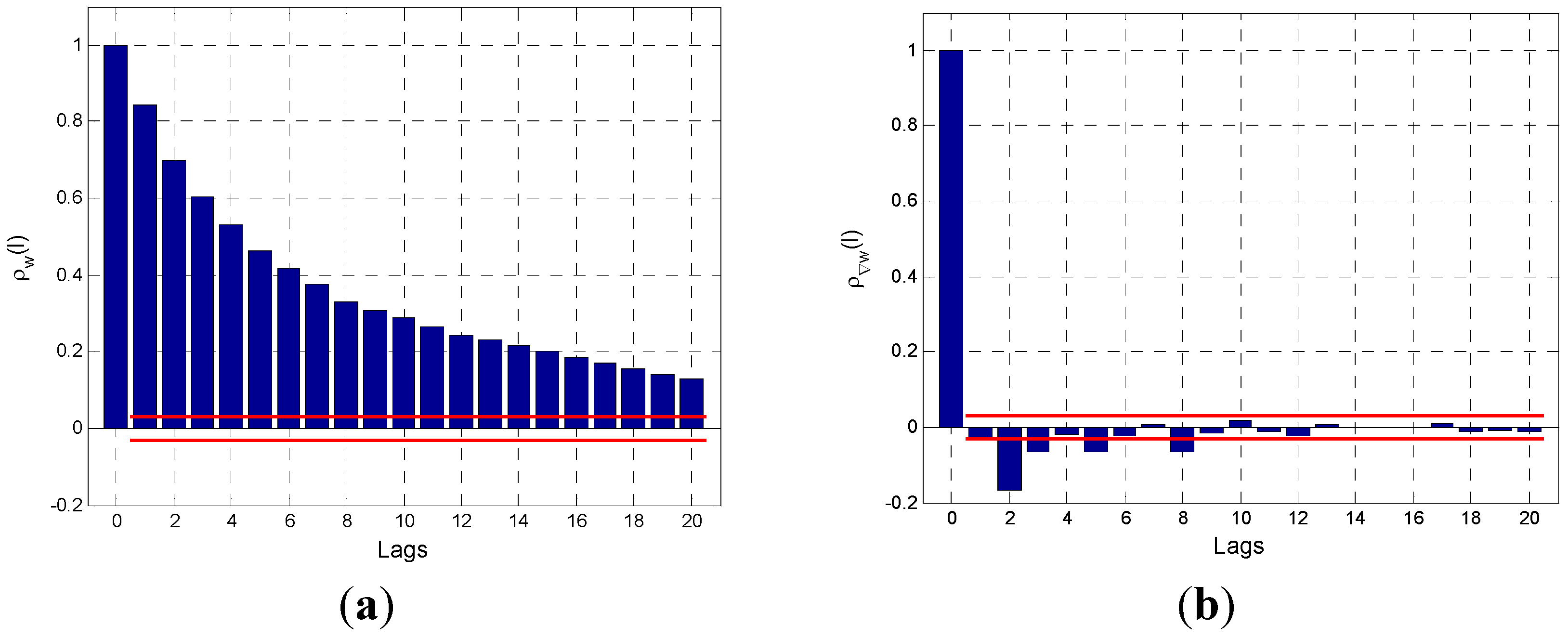
The first step of the Box-Jenkins approach is to identify the degree of differencing,
, exploiting the properties of the autocorrelation functions. In fact, for a stationary time-series, the sample autocorrelation function
quickly decays to zero for moderate lags
, while the non-stationary characteristics in an examined time-series can be observed by the fact that the sample autocorrelation function
decreases very slowly and does not tend to reach zero even for large lags
. This fact suggests that:
if the sample autocorrelation function decreases quickly for increasing values of , the time-series can be represented by a stationary model, and therefore is assumed to be equal to zero;
if the sample autocorrelation function does not decrease quickly for increasing values of , the stochastic process is supposed to be non-stationary in but stationary in for . Specifically, the stochastic process is studied iteratively for ; at each iteration, the autocorrelation function of is investigated, and the iterative process is stopped when the autocorrelation function decreases quickly for increasing values of . Therefore, is assumed to be equal to the number of the iteration that achieved this result; in practice, is normally equal to 1 or 2, and is sufficient to inspect the first 20 estimated autocorrelation coefficients () of the original series and of its first and second differences to determine the value of .
Once the value of the differencing order, is selected, the appropriately-differenced time-series shows characteristics of a stationary process; therefore, it can be modeled by an ARMA process of order . Having built the time-series in such a way, the ARMA process representing and the ARIMA process representing the original time-series share the same orders ; therefore, in the second step of the Box-Jenkins approach, one can study the differenced time-series , and, by fixing the orders of the correspondent ARMA model, the orders of the original ARIMA model also are individuated automatically.
Specifically, in [
26], it was shown that different behaviors of the autocorrelation function
for the differenced series
suggest different values of
, and
Table 1 reports the values for the most common time-series.
Table 1.
Behavior of the sample autocorrelation function, , for the dth difference of an ARIMA process of order .
Table 1.
Behavior of the sample autocorrelation function, , for the dth difference of an ARIMA process of order .
| Order of the ARIMA Model |
|---|
| | | | |
| decreases exponentially | is the only appreciable non-zero term | is a mixture of exponential functions or sine waves | , are the only appreciable non-zero terms | decreases exponentially after |
Once the three orders of the ARIMA process have been determined, a consolidated estimation procedure can be used to obtain estimates of the unknown parameters in Equation (9), which unequivocally identify the time-series model.
In this paper, the parameters of the ARIMA model were evaluated by minimizing the unconditional log-likelihood function of samples of
via the unconditional least squares estimates reported in [
26].
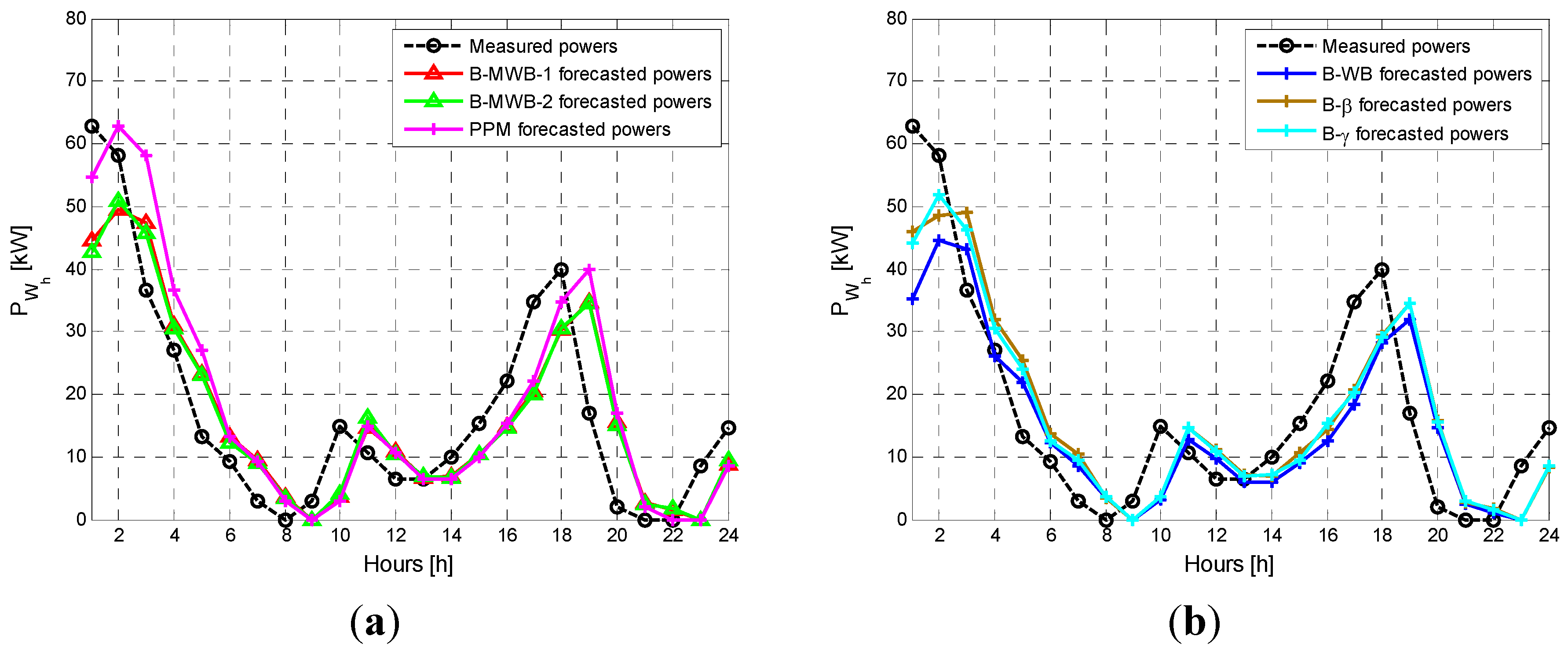
Here, the stochastic variable, was assumed to be the wind speed, . Moreover, once the minimum mean square error forecast of the wind speed for the time horizon was obtained by using the appropriately-estimated ARIMA model, we assumed it to be the expected value of the forecasted distribution, i.e., the mean value to be included in Equation (5).
2.4. Evaluation of the PDFs of the Parameters
Once the mean value of the distribution at the time horizon
were determined as described in
Section 2.3, the remaining parameters
of the distribution in Equation (4) must be obtained. The BI allows the probabilistic estimation of these parameters, identifying their joint posterior probability distribution, by the inference of an array of observations upon the known (or hypothesized) prior probability distributions of each parameter.
The full procedure that is used is described as follows.
The set , composed of measurements of wind speed observed until the origin time , is provided initially. In addition, the prior distributions of the parameters are chosen.
Let
be the generic parameter whose prior distribution must be provided for the time horizon
h; the parameters of the prior distributions commonly are called hyperparameters. There is a great debate in the relevant literature [
47] concerning how to determine the type of the prior distribution of the parameter
and the corresponding hyperparameters. For example, when little or no prior information is provided on the parameter
, an uninformative distribution, such as Jeffreys prior or uniform distribution, is commonly used. However, when some prior statistical information is provided on the parameter
, an informative, appropriate distribution can be used, such as the Gaussian PDF with hyperparameters
.
The main advantage of the Gaussian distribution is the simplicity of the operations in that only the estimates of two hyperparameters are needed, and one can fix the variance
immediately on the basis of her or his confidence in the estimate of the mean value
; a large variance yields a larger, more uniform distribution around the mean value, while a small variance yields a distribution that is more concentrated around the mean value. Coherently, with the behavior of uninformative distributions, specifying a large variance
ensures that the historical data used for the inference determines the relevant changes in the posterior distribution of
to a greater extent than the prior distribution [
47].
In this paper, an initial estimation
was performed for each time horizon
for each parameter
, by applying the well-known moment estimation procedure [
48] on the set of observations of wind speed
. Then, the resulting value of each estimate was assumed to be equal to the mean value of the corresponding prior informative Gaussian distribution,
i.e.,
; then, the variance was assumed to be very high (
for each parameter
, as in [
23]) in order to ensure that the historical data used for the inference, more than the prior distribution, determines the relevant changes in the posterior distribution of parameters.
Instead, for the parameter , a completely uninformative uniform distribution in the interval from to was chosen due the restricted domain in which the parameter is defined.
Now, let be the random parameter vector to be estimated for each time horizon in the BI approach.
Once the prior distributions are set, the BI allows the estimation of the joint posterior distribution, given the set of measurements , through the extension of the Bayes’ Theorem. Unfortunately, a closed-form expression of cannot be provided analytically, but the expression of the un-normalized posterior distribution, , which is directly proportional to , is sufficient for the probabilistic estimation of the parameters.
We can calculate the un-normalized posterior distribution
of the random parameters by:
where
is the likelihood function; and
is the prior distribution of the
th prior random parameter of the vector
. The likelihood function
in Equation (12) is given by:
where
is the Equation (5) evaluated in correspondence to parameters
and
, where
is the minimum mean square error forecast [
26] drawn from the selected ARIMA
model for the time horizon
, given the past
values of wind speed
contained in the set
.
The explicit expression of the likelihood function can be provided in the following form:
Numerical values of Equation (12) can be obtained through different methods that have been extensively used in Bayesian relevant literature [
22,
47,
49,
50]. In this paper, the Monte Carlo Markov Chain simulation method based on the Metropolis-Hasting algorithm was used to obtain samples of the posterior distributions of the parameters in
from the evaluation of the un-normalized posterior distribution
[
22,
47,
49,
50]. Moreover, the size
of the historical data can be selected with adequate criteria, thus improving the accuracy of the forecasting method.


