Life is Short: The Impact of Power States on Base Station Lifetime ^†

Abstract

We study the impact of power state transitions on the lifetime of base stations (BSs) in mobile networks. In particular, we propose a model to estimate the lifetime decrease/increase as a consequence of the application of power state changes. The model takes into account both hardware (HW) parameters, which depend on the materials used to build the device, and power state parameters, that instead depend on how and when power state transitions take place. More in depth, we consider the impact of different power states when a BS is active, and one sleep mode state when a BS is powered off. When a BS reduces the power consumption, its lifetime tends to increase. However, when a BS changes the power state, its lifetime tends to be decreased. Thus, there is a tradeoff between these two effects. Our results, obtained over universal mobile telecommunication system (UMTS) and long term evolution (LTE) case studies, indicate the need of a careful management of the power state transitions in order to not deteriorate the BS lifetime, and consequently to not increase the associated reparation/replacement costs.

1. Introduction

Cellular networks are intensely deployed in the whole world, with different technologies adopted, ranging from legacy 2G networks, to 3G and 4G ones. Focusing on a single base station (BS), its downlink power depends on the number of terminals connected to it, their signal to interference plus noise ratio, as well as the amount of received power for each terminal. In the literature, different solutions have been proposed so far to adjust the power radiated by a BS (see for example [1]). The goal is to guarantee capacity to the users associated with a BS, and also to reduce the overall interference with the neighboring BSs (see e.g., the survey [2]). In this context, resource allocation and interference mitigation are investigated in [3,4,5].

At the same time, power consumption consumed by a single BS is far to be negligible [6]. Moreover, the total power consumption of a BS is influenced by the radiated transmit power [7]. These facts, coupled also with the high number of deployed BSs in an operator network, have stimulated researches towards the reduction of power consumption in cellular networks. One of the most promising approaches to save energy in a cellular network is the exploitation of a sleep mode (SM) state to BSs. More in depth, a BS is completely powered off during low traffic hours (e.g., during night). At the same time, both coverage and traffic requirements are guaranteed by the neighboring BSs that remain powered on. The efficacy and efficiency of BS SM has been extensively studied by previous work (see for example the survey [8]).

A power state transition may therefore occur either when a BS passes from full power to SM (and vice-versa), or when the radiated power is varied. The change in the power state may trigger a change on a temperature variation of some of the BS components. As an example, the authors of [9] report that the largest amount of power consumed by a BS is due to the power amplifier, which is involved when the SM state is activated/deactivated, and also when the radiated power is varied. Thus, power state changes triggering a temperature variation of BS components are affecting the everyday life of a BS. However, some natural questions arise: How do SM and radiated power impact a BS lifetime? Is it possible to build a model to predict the lifetime increase/decrease of a BS as a consequence of its power state change? What is the trade-off between energy savings on one side and reparation/replacement costs on the other? The answer to these questions is the goal of this paper. In particular, we first consider the main effects triggered by the temperature change on a BS. We then build a simple model to compute the lifetime increase/decrease of a BS as a consequence of the application of different power states (i.e., a change in the radiated power, or a SM activation/deactivation). More in depth, when a BS reduces its radiated power or it is put in SM, its lifetime tends to increase, since the temperature of its components is reduced. However, the power state change (either from full power to SM or among different values of radiated power) triggers a negative effect which tends to decrease the lifetime. The combination of these two effects then leads to the variation of the total lifetime experienced by a BS. Finally, we evaluate the proposed model on different realistic case-studies, exploiting 3G and 4G technologies.

Our results indicate that the BS lifetime may be negatively affected when power state transitions take place. This reduction of lifetime will deteriorate the reliability of the network (due to the fact that BSs increase their failure rate), as well as bringing to an increase in the reparation and replacement costs. Therefore, we argue that the lifetime should be considered in the process of deciding how and when to change from a power state to another one. However, we show that the lifetime depends on the hardware (HW) components used to build the device. The goal of this work is also to show the impact on the lifetime due to the behaviour of HW solicited by state transitions, and to stimulate future research in this field, i.e., estimating the values of HW parameters from real measurements.

The rest of the paper is organized as follows. Related works are presented in Section 2. The main effects related to temperature impacting the BS lifetime are summarized in Section 3. Section 4 then presents our model for estimating the BS lifetime. Section 5 details our considered scenarios. Results, obtained from realistic case studies, are reported in Section 6. Section 7 discusses our findings. Finally, Section 8 concludes our work.

2. Related Work

In the literature, different works have investigated the adoption of energy-aware management in cellular networks (see e.g., [10,11,12] for comprehensive surveys). In particular, one of the most promising approaches to save energy in a cellular network is the adoption of SMs. When a BS is in SM, the traffic is served by the neighboring BSs that remain powered on [13]. The problem can be centrally solved [14], i.e., one central node computing the power state for BSs, or in a distributed way [15], i.e., each BS decides when and how to go in SM. Moreover, each BS that remains powered on may increase its power in order to cover the users previously served by BSs that are currently in SM [16], or adopting smart technologies, like coordinated multipoint, to guarantee user coverage and capacity constraints [17]. All these works prove the efficacy of cellular networks in terms of energy, without considering the impact on the lifetime.

Even though the topic of energy-aware cellular networks has been deeply studied in the past years, the application of smart energy-aware policies in real networks is only at the early stage. In particular, one of the main concerns of mobile network operators is the impact of these approaches on the equipment failure rate. The reason is quite simple: since cellular components are not designed to be powered off/on very frequently, the increase in the number of power state transitions triggered by energy-aware policies may negatively impact the equipment lifetime, leading to an increase in the failure rate. In [18] authors consider the limitation of power switching states per day, while at the same time allowing energy savings. However, as we will show in this paper, the lifetime is not merely a function of the number of power state transitions, but it depends on multiple parameters, ranging from the duration of each power state, the characterstics of HW components used to build a BS, the specific time at which the transition takes place, and the scenario taken under consideration (i.e., universal mobile telecommunication system (UMTS) or long term evolution (LTE). In this context, it becomes clear that it is of mandatory importance of investigating failure rate models in energy-aware networks.

Failures in cellular networks are in general very negative events, due to two main reasons: (i) the quality of service (QoS) degradation experienced by users; and (ii) the costs incurred for repairing/replacing the failed equipment. In particular, telecommunication networks are actually experiencing failures during the daily operation of the network (i.e., without energy-aware approaches applied) [19,20], and a failure increase would be therefore unacceptable.

Motivated by these issues, in [21] we have investigated the impact of SM approaches in cellular networks. However, the contribution of radiated power is not taken into account, and the results are obtained only from a 3G network. Additionally, in [22] we have performed a preliminary investigation on the impact of lifetime considering also the active power states. We are not aware of other works on lifetime modeling in green cellular networks. In this work, we go three steps further with respect to previous work by: (i) considering different models for the failure rates (i.e., a linear and an exponential model); (ii) evaluating the impact on the lifetime on the single BSs in a network; and (iii) considering the cost analysis of energy savings vs. reparation and replacement costs over time. We believe that these improvements are of fundamental importance to capture the impact of power state transitions on the lifetime of cellular networks.

Finally, it is worthwhile to mention the national project LIFETEL (increasing the LIFE time of TEL ecommunication networks) [23] which actually supported this work. The goal of LIFETEL is to evaluate the lifetime in telecommunication networks adopting energy-efficient approaches, and to propose new solutions to limit the lifetime decrease, or (possibly) to increase it. The project ranges from backbone to cellular networks, with the aim of giving new directions in the management of lifetime-aware architectures.

3. Impact of Temperature on a Base Station Lifetime

A first order model to compute the failure rate ${\mathsf{\gamma }}^{\mathcal{T}}$ of a device given its temperature $\mathcal{T}$ is the Arrhenius law [24]:

$${\mathsf{\gamma }}^{\mathcal{T}}={\mathsf{\gamma }}^0{e}^{-\frac{E_a}{K\mathcal{T}}}\text{[1/h]}$$

(1)

where ${\mathsf{\gamma }}^0$ is the failure rate estimated assuming a very high temperature, $E_a$ is the activation energy (i.e., the minimum energy needed to activate the failure variation) and K is the Boltzmann constant. Interestingly, when the temperature decreases, the failure rate decreases too. Although more detailed models than the one reported in Equation (1) have been proposed in the literature (see for example [25]) all of them predict a decrease in the failure rate when the temperature is reduced. This means that, if the reduction of the temperature were the only effect taken under consideration, keeping a BS in a low-power state for the longest amount of time would be of benefit for its lifetime.

In addition, a device may suffer strain and fatigue when temperature conditions change, in particular when this happens in a cyclic way (i.e., from one temperature to another one). The Coffin-Manson model [26] describes the effects of material fatigue caused by cyclic thermal stress. The predicted failure rate ${\mathsf{\gamma }}^{{\Delta }_{\mathcal{T}}}$ due to the thermal cycling effect is then expressed as:

$${\mathsf{\gamma }}^{{\Delta }_{\mathcal{T}}}=\frac{f^{\mathrm{TC}}}{N^{\mathrm{f}}}\text{[1/h]}$$

(2)

where $f^{\mathrm{TC}}$ is the frequency of thermal cycling and $N^{\mathrm{f}}$ is the number of cycles to failure. The term $N^{\mathrm{f}}$ is commonly denoted as:

$$N^{\mathrm{f}}=C_0{({\Delta }_{\mathcal{T}}-{\Delta }_{{\mathcal{T}}_0})}^{-q}$$

(3)

where ${\Delta }_{\mathcal{T}}$ is the temperature variation of the cycle, ${\Delta }_{{\mathcal{T}}_0}$ is the maximum admissible temperature variation without a change in the failure rate, $C_0$ is a constant material dependent, q is the Coffin-Manson exponent. From this model, we can clearly see that the more often a device experiences a temperature variation, the higher will be also its failure rate. In the following, we build a model to capture this effect and also to consider the impact of Equation (1).

4. Base Station Lifetime Model

In our work, we consider the BS as a single HW entity. More in depth, we derive a model to express the failure rate of an entire BS. Clearly, this model is an approximation of the real BS behavior, due to the fact that a BS is composed of different HW components, which may exhibit different failure rates. However, our model is able to capture the macroscopic behavior of a system like a complete BS, in order to provide first order insights. We leave the definition of more detailed (and complex) models considering the single BS components as future work.

We start from the assumption that each BS in the network may choose one power state among a discrete set of values. The total BS power is composed by two terms [6]: the static power, that has to be counted if the BS is not in SM, and the dynamic power, which instead depends on the radiated power. In particular, we assume a set of $\mathcal{P}$ power states whose cardinality is $K=\left|\mathcal{P}\right|$. Let us denote with $P_1$,$P_2$,...,$P_{K-1}\in \mathcal{P}$ the power consumed by the BS for dynamic power with indexes 1,2,...,$(K-1)$, respectively. Moreover, $P_{\text{off}}\in \mathcal{P}$ is the power consumed when the BS is in SM state. The power states are ordered in increasing order, i.e., $P_{\text{off}}<P_1<P_2<P_{K-1}$.

For each power state, we denote as ${\mathsf{\tau }}_{\text{off}},{\mathsf{\tau }}_1$,${\mathsf{\tau }}_2$,...,${\mathsf{\tau }}_{K-1}$ the time spent by the BS in power state $P_{\text{off}}$,$P_1$,$P_2$,...,$P_{K-1}$, respectively. The total amount of time under consideration is denoted with T. Moreover, we associate a failure rate to each power state: ${\mathsf{\gamma }}_{\text{off}}$,${\mathsf{\gamma }}_1$,${\mathsf{\gamma }}_2$,...,${\mathsf{\gamma }}_{K-1}$.

The average BS failure rate ${\mathsf{\gamma }}_{\text{s}}$ considering only the impact of different power states is then defined as:

$${\mathsf{\gamma }}_{\text{s}}={\mathsf{\gamma }}_{\text{off}}\frac{{\mathsf{\tau }}_{\text{off}}}{T}+\sum _{i=1}^{K-1}{\mathsf{\gamma }}_i\frac{{\mathsf{\tau }}_i}{T}\text{[1/h]}$$

(4)

which is the sum of the different failure rates, weighed by the normalized amount of time spent in each power state.

In the following, we consider the impact of the thermal cycling effect on the failure rate, which is triggered by the power state transitions. In particular, we denote with ${\mathsf{\delta }}_{i-j}$ the failure rate triggered by the transition between the power state i and the power state j. Similarly, we denote as ${\mathsf{\delta }}_{\text{off}-j}$ the failure rate when passing between the SM state and the power state j. By assuming that the amount of time required for passing from one power state to another one does not influence the failure rate, we express the failure rate ${\mathsf{\delta }}_t$ due to power state transitions as:

$${}_t=\sum _{j=1}^{K-1}{\mathsf{\delta }}_{\text{off}-j}+\sum _{i=1}^{K-1}\sum _{j>i}^{K-1}{\mathsf{\delta }}_{i-j}\text{[1/h]}$$

(5)

The total average failure rate of BS ${\mathsf{\gamma }}_{\text{tot}}$ is then the sum of the failure rates considering the different power states and the failure rates due to power state transitions:

$${\mathsf{\gamma }}_{\text{tot}}={\mathsf{\gamma }}_{\text{s}}+{\mathsf{\delta }}_t\text{[1/h]}$$

(6)

${\mathsf{\gamma }}_{\text{tot}}$ is the sum of failure rates as we have assumed that the failure rates due to the different effects are statistically independent from each other [27].

In the literature, it is common to evaluate the increase/decrease of the current failure rate ${\mathsf{\gamma }}_{\text{tot}}$ with respect to a reference failure rate ${\mathsf{\gamma }}_{\text{tot}}^{\text{ref}}$. This metric is called acceleration factor (AF) [26], which we denote as:

$$AF=\frac{{\mathsf{\gamma }}_{\text{tot}}}{{\mathsf{\gamma }}_{\text{tot}}^{\text{ref}}}$$

(7)

In particular, if the current failure rate is lower than the reference failure rate, the $AF$ is lower than one, and therefore the lifetime is increased. On the contrary, if the $AF$ is greater than one, the lifetime is decreased. Ideally, the $AF$ should be always kept below one. By moving ${\mathsf{\gamma }}_{\text{tot}}^{\text{ref}}$ inside Equation (6) we can express $AF$ as:

$$AF=A{F}_{\text{s}}+A{F}_t$$

(8)

where $A{F}_{\text{s}}={\mathsf{\gamma }}_s/{\mathsf{\gamma }}_{\text{tot}}^{\text{ref}}$ is the acceleration factor due to the time spent in different power states, while $A{F}_t={\mathsf{\delta }}_t/{\mathsf{\gamma }}_{\text{tot}}^{\text{ref}}$ is the acceleration factor due to power state transitions.

We can express the term $A{F}_{\text{s}}$ as:

$$A{F}_{\text{s}}=\underset{\text{SM}}{\underbrace{A{F}_{\text{off}}\frac{{\mathsf{\tau }}_{\text{off}}}{T}}}+\underset{\text{radiated power}}{\underbrace{{\sum }_{i=1}^{K-1}\left[A{F}_i\frac{{\mathsf{\tau }}_i}{T}\right]}}$$

(9)

where $A{F}_{\text{off}}={\mathsf{\gamma }}_{\text{off}}/{\mathsf{\gamma }}_{\text{tot}}^{\text{ref}}$ is the acceleration factor in SM, which is always lower than one since we have assumed that the SM failure rate is lower compared to the reference one. Similarly, $A{F}_i={\mathsf{\gamma }}_i/{\mathsf{\gamma }}_{\text{tot}}^{\text{ref}}$ is the acceleration factor in power state i, which is again lower or equal than one since the failure rate at power state i is always lower or equal than the reference one. Moreover, since the failure rate at power state i is lower than the one at state $(i+1)$, it holds that: $A{F}_{\text{off}}<A{F}_1<A{F}_2<...<A{F}_{K-1}\le 1$.

We then consider the second term $A{F}_t$ of Equation (8). According to Equation (2), the failure rate due to power transitions between state i and state j can be defined as ${\mathsf{\delta }}_{i-j}=\frac{f_{i-j}}{N_{i-j}^f}$, where $f_{i-j}$ is the frequency of power switching between the states and $N_{i-j}^f$ is the maximum number of cycles between state i and state j before a failure occurs. The ratio between ${\mathsf{\delta }}_{i-j}$ and ${\mathsf{\gamma }}_{\text{tot}}^{\text{ref}}$ is then defined as:

$$\frac{{\mathsf{\delta }}_{i-j}}{{\mathsf{\gamma }}_{\text{tot}}^{\text{ref}}}={\chi }_{i-j}^{\text{ref}}{f}_{i-j}$$

(10)

where ${\chi }_{i-j}^{\text{ref}}=\frac{1}{N_{i-j}^f{\mathsf{\gamma }}_{\text{tot}}^{\text{ref}}}$ is the weight for power state frequency $f_{i-j}$. The acceleration factor due to power state transitions is then defined as:

$$A{F}_t=\underset{\text{SM}}{\underbrace{{\sum }_{j=1}^{K-1}{\chi }_{\text{off}-j}^{\text{ref}}{f}_{\text{off}-j}}}+\underset{\text{radiated power}}{\underbrace{{\sum }_{i=1}^{K-1}{\sum }_{j>i}^{K-1}\left[{\chi }_{i-j}^{\text{ref}}{f}_{i-j}\right]}}$$

(11)

$A{F}_t$ may assume values larger than one, since both $f_{\text{off}-j}$ and $f_{i-j}$ may be larger than one (especially when different power state transitions occur during the time period T). As a consequence, this term tends to increase the total acceleration factor and therefore to decrease the BS lifetime.

We now consider the different parameters included in the $AF$ metric. In particular, the weights ${\chi }_{\text{off}-j}^{\text{ref}}$ and ${\chi }_{i-j}^{\text{ref}}$ are depending on the HW characteristics, i.e., they are fixed given the reference failure rate and the number of cycles to failures. Similarly, also the terms $A{F}_{\text{off}}$ and $A{F}_i$ may be known by measuring the failure rate at a given power value. On the contrary, the terms ${\mathsf{\tau }}_{\text{off}}$ and $f_{\text{off}-j}$ depend on the implementation of the SM approach. In practice, these terms need to be carefully planned by taking into account the current BS and the neighboring ones, i.e., to avoid a coverage hole or an overloading of the neighboring BSs. Similarly, the terms ${\mathsf{\tau }}_i$ and $f_{i-j}$ depends instead on the policy to allocate power to users, which is influenced by the number of active terminals and their rate requirements.

Since both SMs and power allocation states are varied considering a set of BSs as a whole, an operator might be interested to observe the acceleration factor over the set of BSs $\mathcal{Z}$. In particular, we can define the average AF as:

$$A{F}^{\text{tot}}=\frac{{\sum }_{z}A{F}^z}{\left|\mathcal{Z}\right|}$$

(12)

where $A{F}^z$ is the acceleration factor of BS z computed with Equation (8). Intuitively, if $A{F}^{\text{tot}}<1$, BSs in the network fail less often compared to the reference failure rate, and therefore the average lifetime tends to be increased. On the contrary, when $A{F}^{\text{tot}}>1$ the lifetime tends to be decreased. Similarly, the operator might be interested to observe the worst case acceleration factor, i.e., $A{F}^{\text{max}}={max}_{z}A{F}^z$.

4.1. Base Station Hardware Parameters Setting

The BS lifetime model takes as input the power state transitions parameters, which depend on the policy used to change BS power, and HW parameters, which instead depend on the components used to build the BS. The following subsections detail the BS HW parameters setting, considering a linear model and an exponential model, respectively.

4.1.1. Linear Model

We first assume that the reference failure rate ${\mathsf{\gamma }}_{\text{tot}}^{\text{ref}}$ is the one obtained when a BS transmits at maximum power, i.e., 40 W [28]. ${\mathsf{\gamma }}_{\text{tot}}^{\text{ref}}$ is normalized to one for simplicity. The actual BS lifetime will be then computed in Section 6.3. Our goal is then to compute the BS AF over the whole day under consideration. To this extent, we have to sum the acceleration factor due to the time spent in different power states ($A{F}_{\text{s}}$ of Equation (9)) and the one due to power state transitions ($A{F}_t$ of Equation (11)).

Focusing on $A{F}_{\text{s}}$, we report in Table 1 the $A{F}_i$ parameters for the active power states. In particular, we assume that the values of $A{F}_i$ are linearly chosen between $1-\frac{(1-A{F}_{\text{off}})}{2}$ (which corresponds to the AF experienced when the BS transmits at 10 W) and 1 (which corresponds to the maximum transmission power). The reason for choosing such values is the following. First, the maximum AF is the one at full power, which is taken as reference in our scenario. Second, the minimum $A{F}_i$ (when the power is equal to 10 W) is always much larger than $A{F}_{\text{off}}$, since we expect that even with radiated power equal to 10 W a large amount of components has to be powered on, leading to a higher failure rate w.r.t. the SM case.

Table 1. $A{F}_i$ values for each power state — linear model.

Power state	${\mathrm{P}}_1$ (10 W)	${\mathrm{P}}_2$ (20 W)	${\mathrm{P}}_3$ (30 W)	${\mathrm{P}}_4$ (40 W)
$A{F}_i$	$1-\frac{(1-A{F}_{\text{off}})}{2}$	$1-\frac{(1-A{F}_{\text{off}})}{3}$	$1-\frac{(1-A{F}_{\text{off}})}{6}$	1

Table 1. $A{F}_i$ values for each power state — linear model.

Power state	${\mathrm{P}}_1$ (10 W)	${\mathrm{P}}_2$ (20 W)	${\mathrm{P}}_3$ (30 W)	${\mathrm{P}}_4$ (40 W)
$A{F}_i$	$1-\frac{(1-A{F}_{\text{off}})}{2}$	$1-\frac{(1-A{F}_{\text{off}})}{3}$	$1-\frac{(1-A{F}_{\text{off}})}{6}$	1

As next step, we consider the AF due to power state transitions ($A{F}_t$). Since the setting of all the frequency weights χ in Equation (11) would be very challenging in practice, we assume that: (i) the same weight ${\chi }_{\text{ref}}^{\text{off}}$ is paid when passing from each active power state to SM (and vice-versa); (ii) the same weight is paid when the same difference in terms of radiated power occurs (e.g., from 10 W to 20 W, or from 20 W to 30 W); (iii) the weight paid when the radiated power is changed is much lower compared to ${\chi }_{\text{ref}}^{\text{off}}$. Table 2 reports the adopted frequency weights, together with the corresponding notation for denoting the frequency (e.g., $F_1$ accounts for all the transitions involving a change in the radiated power equal to 10 W). As such, the term $A{F}_t$ is computed as follows: $A{F}_t=W{\chi }_{\text{ref}}^{\text{off}}{\sum }_{k=1}^{3}k{F}_k+{\chi }_{\text{ref}}^{\text{off}}{F}_{\text{off}}$, being W a small value ($W<<1$). The reasons for choosing these settings are the following ones. First, we assume that BS components are optimized to limit the thermal cycling effect triggered by radiated power variations. Therefore, we have set the frequency weights in such a way that they are always much smaller than ${\chi }_{\text{ref}}^{\text{off}}$ (by setting the W parameter). Second, we expect that the highest failure rate change is triggered when the BS enters/leaves a SM state, which justifies the same weight paid when passing from an active power state to SM. Third, as reported in Equations (2) and (3) the most important factor impacting the thermal cycling effect is the difference in temperature between two power states (and not their absolute values). This fact motivates the adoption of a frequency weight based on the difference in power (i.e., off, 10 W, 20 W or 30 W).

Table 2. Frequency notation and frequency weight for each power variation—linear model.

Power variation	Off	10 W	20 W	30 W
Frequency notation	$F_{\text{off}}$	$F_1$	$F_2$	$F_3$
Frequency weight	${\chi }_{ref}^{\text{off}}$	$W{\chi }_{\text{ref}}^{\text{off}}$	$2W{\chi }_{\text{ref}}^{\text{off}}$	$3W{\chi }_{\text{ref}}^{\text{off}}$

Table 2. Frequency notation and frequency weight for each power variation—linear model.

Power variation	Off	10 W	20 W	30 W
Frequency notation	$F_{\text{off}}$	$F_1$	$F_2$	$F_3$
Frequency weight	${\chi }_{ref}^{\text{off}}$	$W{\chi }_{\text{ref}}^{\text{off}}$	$2W{\chi }_{\text{ref}}^{\text{off}}$	$3W{\chi }_{\text{ref}}^{\text{off}}$

Summarizing, we are now able to compute the AF for a single BS $A{F}^z$, leaving $A{F}_{\text{off}}$, ${\chi }_{\text{ref}}^{\text{off}}$ and W as HW input parameters. Figure 1 reports the main steps to obtain $A{F}^z$. In particular, we start from a traffic variation over time, and scenario constraints (e.g., coverage, capacity). Given these input parameters, we compute the set of power states over time adopting an energy-aware approach, i.e., a solution which tends to assign the minimum power consumption to satisfy the constraints. We then compute the power state transitions parameters (i.e., ${\mathsf{\tau }}_{\text{off}}$, ${\mathsf{\tau }}_i$, $F_{\text{off}}$, $F_1$, $F_2$, $F_3$) which take into account the duration of power states and their transitions rate. Given these parameters and the HW parameters (namely $A{F}_{\text{off}}$, ${\chi }_{\text{ref}}^{\text{off}}$ and W), we compute with our model the BS AF (and consequently the lifetime).

Figure 1. Main steps to compute the AF for the z-th base station (BS) in the network.

Figure 1. Main steps to compute the AF for the z-th base station (BS) in the network.

From now on, we assume that the BSs in the considered scenarios have the same HW characteristics, i.e., $A{F}_{\text{off}}$, W, and ${\chi }_{\text{ref}}^{\text{off}}$ are the same for all the BSs. Clearly, in case of different HW parameters, the effects for applying power state transitions will be not the same for all BSs. We leave this aspect for future work.

Table 3 reports the main notation introduced so far.

4.1.2. Exponential Model

We consider also an exponential model for setting the AF and the frequency weight values in active power states. The reason for this model is that, actually, there are not available measurements for expressing the HW parameters. Thus, our aim is to investigate the impact of different models for estimating the lifetime given the power state variations. In particular, the exponential model may be adopted for devices which are less susceptible to power state changes compared to the linear one. At the same time, the gain for exploiting low power states (in active mode) is higher w.r.t. the linear model. 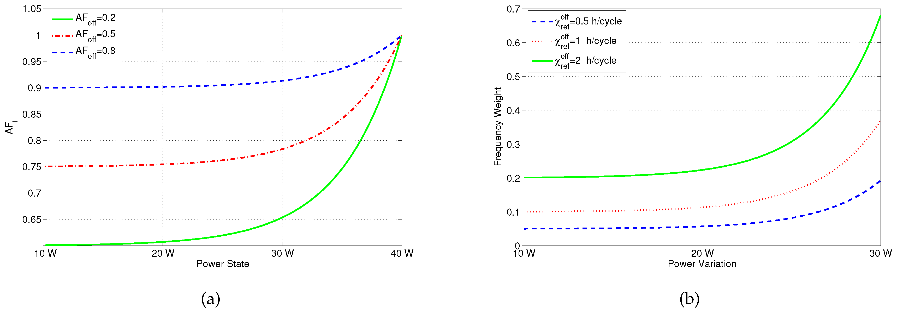Figure 2 reports the parameters set for the $A{F}^i$ and the frequency weight values, respectively. Focusing on the $A{F}_i$ values (reported in Figure 2a) we can see that a good gain in the AF can be reached by setting 30 W compared to the 40 W case. Focusing then on the frequency weight values (reported in Figure 2b) we can note that power state transitions of 10 W and 20 W basically have the same influence on the AF, while the 30 W case implies a more notable variation of the AF.

Table 3. Main notation.

Symbol	Measurement unit	Description
$\mathcal{P}$	-	Set of power states (active and sleep mode (SM))
K	[units]	number of power states
$P_i$	[Watt]	Power consumed by the base station (BS) in active state $i\in \mathcal{P}$
$P_{\text{off}}$	[Watt]	Power consumed by the BS in SM state
${\mathsf{\tau }}_i$	[h]	Time spent by BS in active state $i\in \mathcal{P}$
${\mathsf{\tau }}_{\text{off}}$	[h]	Time spent by BS in SM state
T	[h]	Total period of time under consideration
${\mathsf{\gamma }}_i$	[1/h]	BS Failure rate in active state $i\in \mathcal{P}$
${\mathsf{\gamma }}_{\text{off}}$	[1/h]	BS Failure rate in SM state
${\mathsf{\gamma }}_{\text{s}}$	[1/h]	BS Failure rate considering only the impact of different power states
${\mathsf{\delta }}_{i-j}$	[1/h]	BS Failure rate when passing between state i and state j
${\mathsf{\delta }}_{\text{off}-j}$	[1/h]	BS Failure rate when passing between SM state and state j
${\mathsf{\delta }}_t$	[1/h]	BS Failure rate due to power state transitions
${\mathsf{\gamma }}_{\text{tot}}$	[1/h]	Total BS failure Rate
${\mathsf{\gamma }}_{\text{tot}}^{\text{ref}}$	[1/h]	Total reference BS failure Rate
$A{F}_{\text{s}}$	[units]	Acceleration factor due to the time spent in different power states
$A{F}_t$	[units]	Acceleration factor due to power state transitions
$AF$	[units]	Total acceleration factor
$A{F}_{\text{off}}$	[units]	Acceleration factor in SM
$A{F}_i$	[units]	Acceleration factor in power state i
$f_{i-j}$	[cycle/h]	Power switching frequency between state i and state j
$N_{i-j}^{\text{f}}$	[cycle]	Number of cycles to failure between state i and state j
$f_{\text{off}-j}$	[cycle/h]	Power switching frequency between SM state and state j
$N_{\text{off}-j}^{\text{f}}$	[cycle]	Number of cycles to failure between SM state and state j
${\chi }_{i-j}^{\text{ref}}$	[h/cycle]	Weight parameter for the power state frequency $f_{i-j}$
${\chi }_{\text{off}-j}^{\text{ref}}$	[h/cycle]	Weight parameter for the power state frequency $f_{\text{off}-j}$
$A{F}^z$	[units]	Acceleration factor for the z-th BS
$\mathcal{Z}$	[units]	Set of BSs in the network
$A{F}^{\text{tot}}$	[units]	Total acceleration factor in the network
W	[units]	Frequency Weight multiplier
${\chi }_{\text{ref}}^{\text{off}}$	[h/cycle]	Weight parameter for a power state frequency between SM and an active sate
$F_{\text{off}}$	[cycle/h]	Frequency for a power transition between SM and an active sate
$F_1$	[cycle/h]	Frequency for a power transition between two active states with 10 W of difference
$F_2$	[cycle/h]	Frequency for a power transition between two active states with 20 W of difference
$F_3$	[cycle/h]	Frequency for a power transition between two active states with 30 W of difference

Table 3. Main notation.

Symbol	Measurement unit	Description
$\mathcal{P}$	-	Set of power states (active and sleep mode (SM))
K	[units]	number of power states
$P_i$	[Watt]	Power consumed by the base station (BS) in active state $i\in \mathcal{P}$
$P_{\text{off}}$	[Watt]	Power consumed by the BS in SM state
${\mathsf{\tau }}_i$	[h]	Time spent by BS in active state $i\in \mathcal{P}$
${\mathsf{\tau }}_{\text{off}}$	[h]	Time spent by BS in SM state
T	[h]	Total period of time under consideration
${\mathsf{\gamma }}_i$	[1/h]	BS Failure rate in active state $i\in \mathcal{P}$
${\mathsf{\gamma }}_{\text{off}}$	[1/h]	BS Failure rate in SM state
${\mathsf{\gamma }}_{\text{s}}$	[1/h]	BS Failure rate considering only the impact of different power states
${\mathsf{\delta }}_{i-j}$	[1/h]	BS Failure rate when passing between state i and state j
${\mathsf{\delta }}_{\text{off}-j}$	[1/h]	BS Failure rate when passing between SM state and state j
${\mathsf{\delta }}_t$	[1/h]	BS Failure rate due to power state transitions
${\mathsf{\gamma }}_{\text{tot}}$	[1/h]	Total BS failure Rate
${\mathsf{\gamma }}_{\text{tot}}^{\text{ref}}$	[1/h]	Total reference BS failure Rate
$A{F}_{\text{s}}$	[units]	Acceleration factor due to the time spent in different power states
$A{F}_t$	[units]	Acceleration factor due to power state transitions
$AF$	[units]	Total acceleration factor
$A{F}_{\text{off}}$	[units]	Acceleration factor in SM
$A{F}_i$	[units]	Acceleration factor in power state i
$f_{i-j}$	[cycle/h]	Power switching frequency between state i and state j
$N_{i-j}^{\text{f}}$	[cycle]	Number of cycles to failure between state i and state j
$f_{\text{off}-j}$	[cycle/h]	Power switching frequency between SM state and state j
$N_{\text{off}-j}^{\text{f}}$	[cycle]	Number of cycles to failure between SM state and state j
${\chi }_{i-j}^{\text{ref}}$	[h/cycle]	Weight parameter for the power state frequency $f_{i-j}$
${\chi }_{\text{off}-j}^{\text{ref}}$	[h/cycle]	Weight parameter for the power state frequency $f_{\text{off}-j}$
$A{F}^z$	[units]	Acceleration factor for the z-th BS
$\mathcal{Z}$	[units]	Set of BSs in the network
$A{F}^{\text{tot}}$	[units]	Total acceleration factor in the network
W	[units]	Frequency Weight multiplier
${\chi }_{\text{ref}}^{\text{off}}$	[h/cycle]	Weight parameter for a power state frequency between SM and an active sate
$F_{\text{off}}$	[cycle/h]	Frequency for a power transition between SM and an active sate
$F_1$	[cycle/h]	Frequency for a power transition between two active states with 10 W of difference
$F_2$	[cycle/h]	Frequency for a power transition between two active states with 20 W of difference
$F_3$	[cycle/h]	Frequency for a power transition between two active states with 30 W of difference

Figure 2. Exponential model: $A{F}^i$ values and frequency weight values. (a) $A{F}^i$ values; (b) frequency weight values.

Figure 2. Exponential model: $A{F}^i$ values and frequency weight values. (a) $A{F}^i$ values; (b) frequency weight values.

5. Scenario Description

We first describe the scenario based on UMTS, and then we consider the LTE case. The reason for choosing these scenarios is to evaluate the impact on the lifetime in both cases, since they are quite different in terms of adopted devices, resource management policies, deployment strategies and algorithms to manage BSs power states.

5.1. Universal Mobile Telecommunication System Scenario

We consider an energy-aware algorithm and a realistic UMTS cellular deployment scenario, both obtained from [29]. We refer the reader to [29] for a comprehensive description. In brief, we consider a scenario with 33 UMTS macro BSs and a service area (SA) of $9.2\times 9.2$ km${}^2$. Each macro BS consumes a fixed amount of power, that has to be counted if the BS is powered on, and a dynamic one, which depends on the radiated power. The radiated power can be set to 10 W, 20 W, 30 W or 40 W, respectively. Inside the SA, we assume more than 3000 user terminals (UTs) requesting voice and data services. Unless otherwise specified, we assume the maximum data rate for each UT is equal to 384 kbps. Moreover, we assume a day-night traffic variation with a periodic profile over the 24 h, with a minimum traffic granularity equal to one hour.

Over such scenario, we solve the optimization problem of minimizing the energy consumption of active BSs while guaranteeing the required coverage and capacity demand for all the UTs which are active in each time period. We refer the reader to [29] for more details about the optimization model and the obtained results. For each BS, we collect the frequency and duration of each power state obtained from the solution of the problem.

5.2. Long Term Evolution Scenario

We assume a hierarchical LTE network in which a single macro provides coverage over the SA, while micro BSs provide capacity in hot-spot areas. The main parameters are reported in Table 4. In particular, the micro BSs are randomly deployed inside the SA. However, in order to prevent micro BSs overlapping, we impose a minimum distance between the micro BSs. Focusing on users, 30% of users are randomly placed inside the SA, while 70% of them are placed close to the micro BSs in order to generate hot-spot zones. Focusing then on user traffic, we assume that users request voice over internet protocol (VoIP), data and web services. More in depth, 10% of users are VoIP, 40% data and 50% web. The service distribution is taken from [30].

Table 4. LTE scenario parameters.

Parameter	Value
Macro BS Radius	1000 m
Number of micro	{10,20,30}
Maximum number of users $N^{\text{max}}$	{227,300,380}
Minimum micro BS distance	200 m
Receiver node power	–97.5 dBm
Min receiver sensitivity	–107.5 dBm
User voice over internet protocol (VoIP) rate	64 kbps
User data rate	0.512–2 Mbps
User web rate	0.064–4 Mbps
Maximum BS TX power	37 dBm (micro), 46 dBm (macro sector)
BS antenna gain	10 dBm (micro), 16 dBm (macro sector)
BS operating frequency	2 GHz
BS bandwidth	5 MHz (micro), 10 MHz (macro)
Number of resource blocks per BS	25 (micro), 50 (macro)

Table 4. LTE scenario parameters.

Parameter	Value
Macro BS Radius	1000 m
Number of micro	{10,20,30}
Maximum number of users $N^{\text{max}}$	{227,300,380}
Minimum micro BS distance	200 m
Receiver node power	–97.5 dBm
Min receiver sensitivity	–107.5 dBm
User voice over internet protocol (VoIP) rate	64 kbps
User data rate	0.512–2 Mbps
User web rate	0.064–4 Mbps
Maximum BS TX power	37 dBm (micro), 46 dBm (macro sector)
BS antenna gain	10 dBm (micro), 16 dBm (macro sector)
BS operating frequency	2 GHz
BS bandwidth	5 MHz (micro), 10 MHz (macro)
Number of resource blocks per BS	25 (micro), 50 (macro)

Walfisch-Ikegami model [31]. The main parameters for this model are reported in Table 5. In brief, we consider an urban scenario where the macro BS is deployed on top of the buildings, while the micro BSs are installed at the intermediate floors. Moreover, users are assumed to be placed at the ground level where no line-of-sight (NLOS) exists.

Table 5. Parameters for the walfisch-ikegami model.

Parameter	Value
BS height	10 m (micro) 23 m (macro)
Average building height	20 m
Average road width	20 m
Average building separation	36 m
Receiver height	1.5 m

Table 5. Parameters for the walfisch-ikegami model.

Parameter	Value
BS height	10 m (micro) 23 m (macro)
Average building height	20 m
Average road width	20 m
Average building separation	36 m
Receiver height	1.5 m

In order to compute the propagation loss between each user and each BS, we adopt the Users are associated to each BS assuming a best server allocation policy. In particular, the allocation of resources to users requests to consider resource blocks (RBs) [32]. More in depth, RBs are assigned first to VoIP users, then to data users, and finally to web ones. Each web user obtains at least one RB, and the remaining RBs available at the end of the procedure are assigned to the web users (ordered with decreasing channel quality indicator (CQI)), until there are RBs available. Finally, we always guarantee the resources to the control channels.

Unless otherwise specified, we consider that the number of users $N_t$ varies over 24 h with a sinusoidal function between $N^{\max }$ and $0.2N^{\max }$, since we assume a day-night behavior [13]. Since our goal is mainly to perform a first order analysis, we vary the number of users with a simple function. The investigation of more complex traffic profiles is left for future work. Additionally, we consider a time-period of 14 days by repeating the variation of the users over the days. Note that while the variation of the number of users is repeated over the days, the actual user placement may be different from one day to another one. The minimum time granularity is set to 1 h.

In order to compute the set of BSs in SM, we consider the least load algorithm (LLA) of [33]. In particular, the original LLA (denoted as LLA-O in the following) always starts with all BSs powered on. Then, BSs are sorted in increasing value of load. For each BS (starting from the least-loaded ones), the current BS is put in SM. If coverage and capacity constraints are satisfied, the BS is kept in SM. Otherwise, the current BS is powered on again. The procedure is repeated for all the BSs. In our case, due to the fact that the LLA-O algorithm always starts with all BSs powered on, there are a lot of power state transitions between the current traffic matrix and the previous one. Therefore, we expect a strong impact on the average AF. In order to be more conservative, we consider an improved version of LLA (denoted as LLA-I in the following). In particular, the LLA-I algorithm works exactly in the same way as the LLA-O one, but we compute in the AF only the transitions between the current network configuration (in terms of BSs powered on) and the previous one. Clearly, LLA-I represents an optimistic scenario, which may be challenging to be implemented in practice.

6. Model Evaluation

We first consider the results derived from the UMTS scenario, then we consider the LTE one, and finally we detail a cost analysis based on the actual lifetime experienced by the BSs in our scenarios.

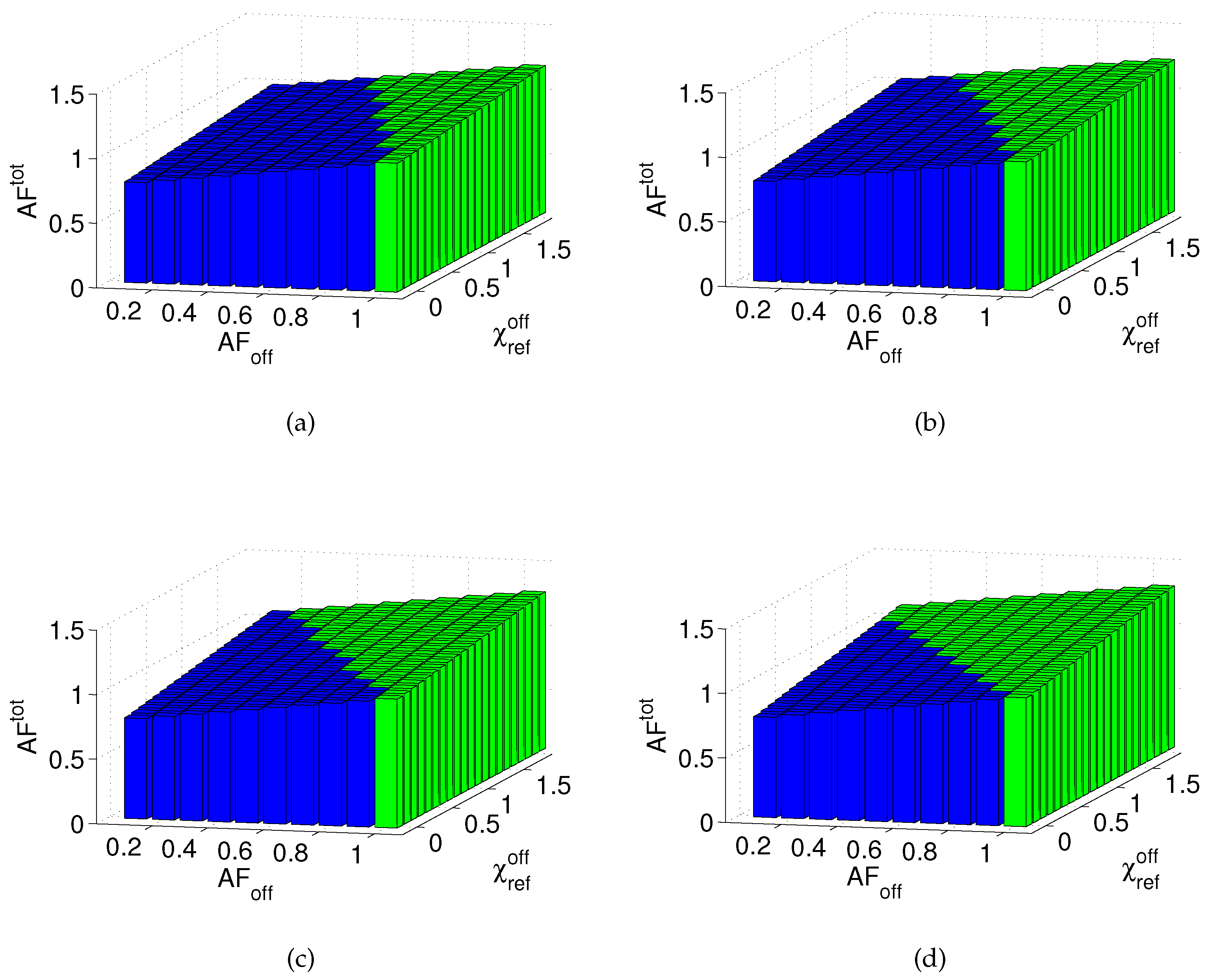
We first compute the total AF in the network $A{F}^{\text{tot}}$ as defined in Equation (12), considering a period of time T equal to 24 h. Figure 3 reports the AF computed considering the variation of HW parameters $A{F}_{\text{off}}$, ${\chi }_{\text{ref}}^{\text{off}}$ and W. From the figure, we can clearly see that as $A{F}_{\text{off}}$ is reduced, $A{F}^{\text{tot}}$ tends to decrease. Ideally, $A{F}_{\text{off}}$ may be equal to zero, meaning that the BS lifetime is increased to infinity when a SM state is set. However, even in this case, the network $A{F}^{\text{tot}}$ is strictly larger than zero since a subset of BSs in the scenario has to be powered on to meet user coverage and capacity constraints. On the contrary, $A{F}^{\text{tot}}$ tends to increase when ${\chi }_{\text{ref}}^{\text{off}}$ is increased. Interestingly, two distinct regions emerge: one with $A{F}^{\text{tot}}<1$ (i.e., increase of lifetime), and one with $A{F}^{\text{tot}}\ge 1$ (i.e., equal lifetime or decrease of lifetime). Thus, power state transitions may even decrease the BS lifetime compared to the case in which BSs always transmit at maximum power. Finally, when W is increased (from left to right subplots), the region in which $A{F}^{\text{tot}}<1$ is promptly reduced. Since in all the cases power state transitions have an impact on the lifetime, we argue that they should be carefully planned, i.e., either to maximize the BS lifetime or to limit the lifetime decrease.

Figure 3. $A{F}^{\text{tot}}$ in the network vs. different values of parameter W (blue bars: $A{F}^{\text{tot}}<1$, green bars: $A{F}^{\text{tot}}\ge 1$). (a) $W=0.05$; (b) $W=0.1$; (c) $W=0.15$; (d) $W=0.2$.

Figure 3. $A{F}^{\text{tot}}$ in the network vs. different values of parameter W (blue bars: $A{F}^{\text{tot}}<1$, green bars: $A{F}^{\text{tot}}\ge 1$). (a) $W=0.05$; (b) $W=0.1$; (c) $W=0.15$; (d) $W=0.2$.

6.1. Universal Mobile Telecommunication System Case-Study Results

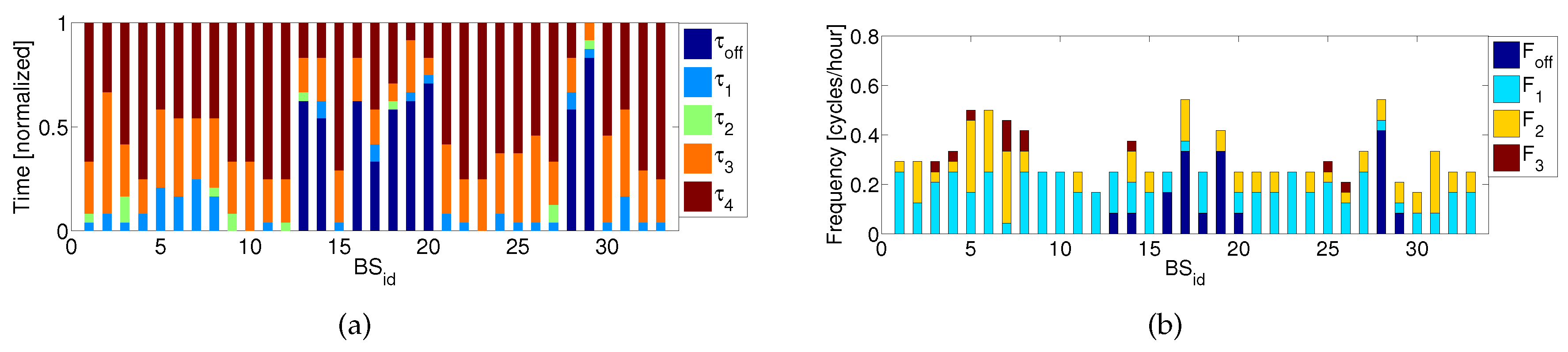
In the next step, we consider the impact of our model on the single BSs. To this extent, Figure 4a reports the normalized time spent in each power state (SM, 10 W, 20 W, 30 W, 40 W). Interestingly, all the BSs tend to use the entire set of available active power states (corresponding to a normalized time spent in ${\mathsf{\tau }}_1$, ${\mathsf{\tau }}_2$, ${\mathsf{\tau }}_3$ and ${\mathsf{\tau }}_4$). This sugggests that the radiated power tends to follow the dynamics of traffic (i.e., the maximum during peak hours and then the minimum during off peak hours). Moreover, the SM state ${\mathsf{\tau }}_{\text{off}}$ is reached by a subset of BSs, since it is not possible to put in SM all the BSs. 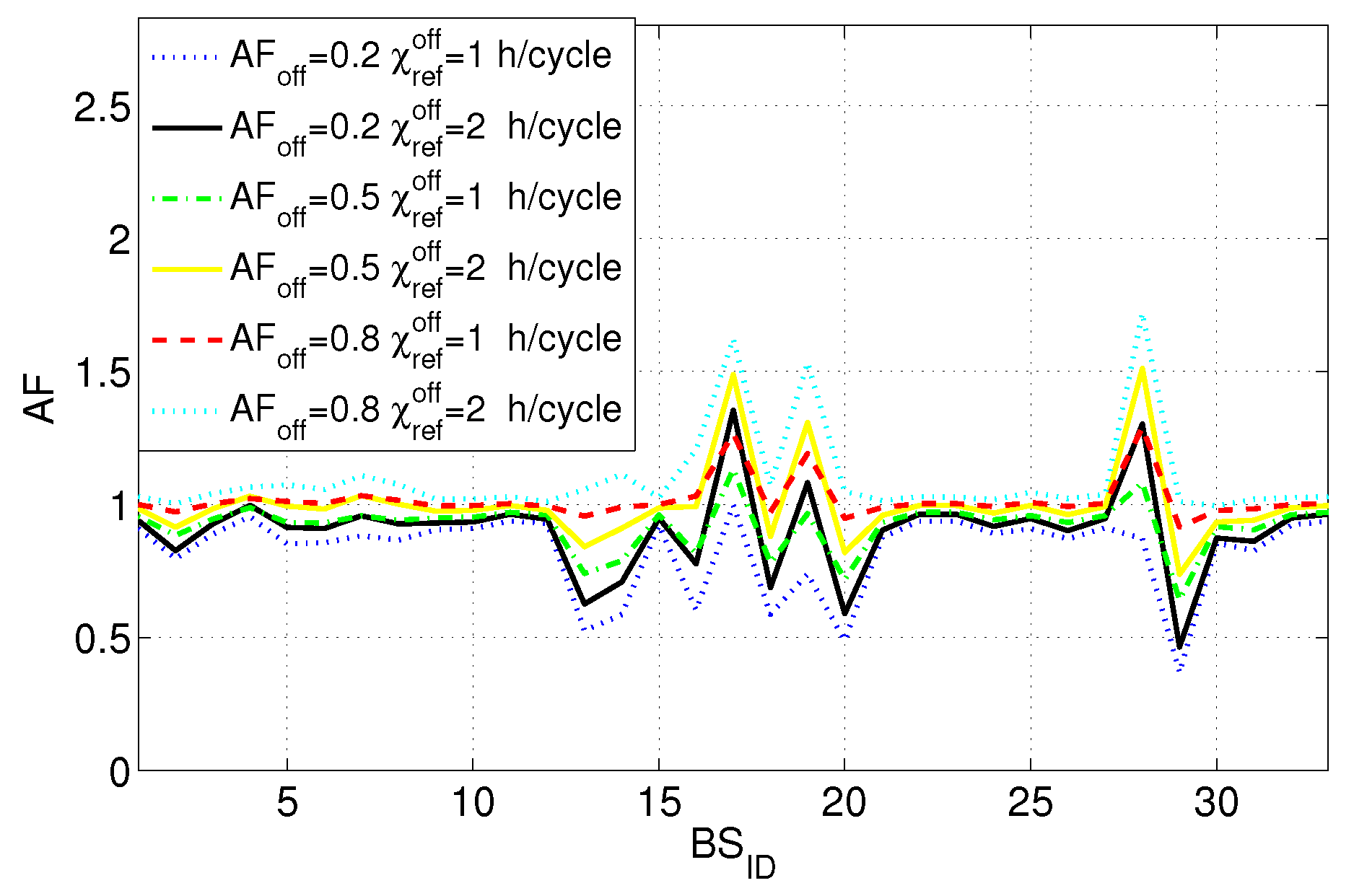To give more insight, Figure 4b reports the frequency of each transition. In this case, most of transitions involve difference of power equal to 10 W and 20 W, while the 30 W variation rarely occurs. 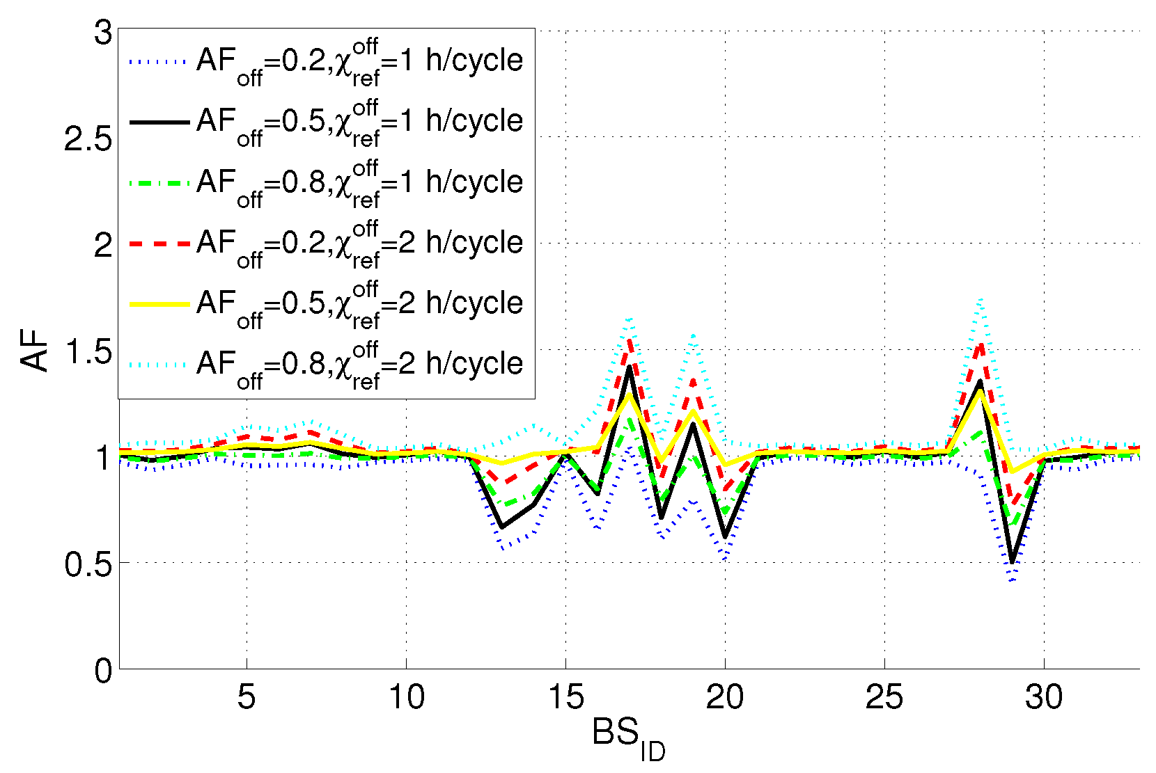More in depth, the frequency $F_{\text{off}}$ of BS 28 and BS 19 is around 0.4 cycles/h, suggesting that these BSs are put in SM and then in active power several times during a day. Additionally, Figure 5 reports the AF for each BS in the network for different values of $A{F}_{\text{off}}$ and ${\chi }_{\text{ref}}^{\text{off}}$. Unless otherwise specified, W is set to $0.1$. Interestingly, we can see that the impact of AF is not the same for all the BSs in the network, with some BSs that tend to steadily increase their AF (e.g., BS 28 has a maximum AF equal to 1.7, which means a lifetime reduction of 70%), and others which instead are able to decrease their AF. Thus, we argue the need of a wise strategy in selecting the power state transitions considering the lifetime of the single BSs.

Figure 4. Normalized time spent in each power state and frequency of power transitions. (a) Normalized time spent in each power state; (b) frequency of power transitions.

Figure 4. Normalized time spent in each power state and frequency of power transitions. (a) Normalized time spent in each power state; (b) frequency of power transitions.

Figure 5. $AF$ for the single BSs in the network.

Figure 5. $AF$ for the single BSs in the network.

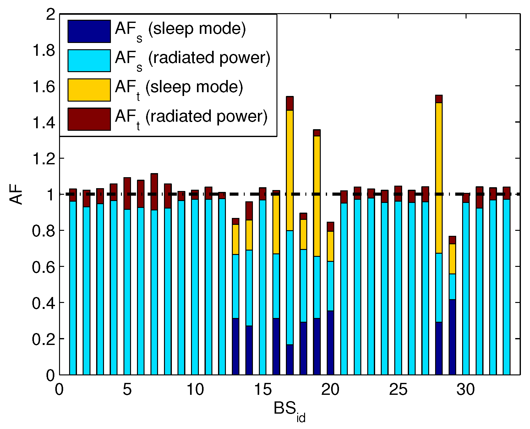
In the following, we focus on the acceleration factor due to the time spent in different power states ($A{F}_{\text{s}}$) and the one due to power state transitions ($A{F}_t$). In this case, we consider $A{F}_{\text{off}}=0.5$, ${\chi }_{\text{ref}}^{\text{off}}=2$ (h/cycle) and $W=0.1$. Figure 6 reports the values of $A{F}_{\text{s}}$ and $A{F}_t$, by differentiating also between the amount due to radiated power and the one due to SM. Interestingly, we can see that the BSs showing the highest total AF are also the ones having the highest $A{F}_t$ in SM, which accounts for the frequency at which BSs enter/leave SM, as well as the HW parameter ${\chi }_{\text{ref}}^{\text{off}}$. The values of $A{F}_s$ on the contrary are always lower than one, due to the fact that $A{F}_{\text{off}}$, $A{F}_i$, ${\mathsf{\tau }}_{\text{off}}/T$ and ${\mathsf{\tau }}_i/T$, are always lower than one. Moreover, we can see that the radiated power has a small impact on $A{F}_t$. However, for some BSs, the term $A{F}_t$ (which depends on the radiated power) tends to bring the overall AF larger than 1, which means a decrease in the lifetime.

Figure 6. $AF$ components in the network.

Figure 6. $AF$ components in the network.

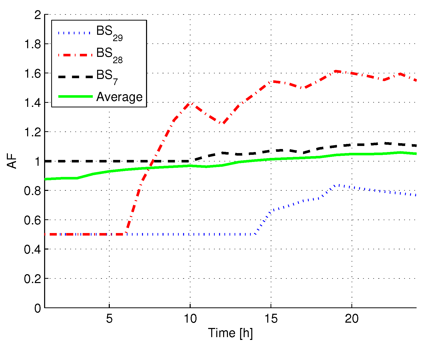
Finally, we have considered how the AF evolves over time. In particular, we have computed the AF for each hour in the network, i.e., starting from 00:00 and computing the AF in the current hour considering the power state variations occurred from 00:00 to the current hour. Figure 7 reports the AF evolution considering $A{F}_{\text{off}}=0.5$, ${\chi }_{\text{ref}}^{\text{off}}=2$ (h/cycle) and $W=0.10$. The figure reports two BSs exploiting SMs ($B{S}_{29}$,$B{S}_{28}$) and one which is always powered on ($B{S}_7$). Interestingly, we can see that the network AF is initially lower than one, then at 11 a.m. it becomes higher than one. This suggests that the energy-aware algorithm has initially decreased the BSs power as a consequence of periods of low traffic. However, since user traffic increases during the following morning hours, different BSs have to change their power state. As a result, the lifetime in the network is decreased at the end of the day. Moreover, the acceleration factor of the single BSs exhibits very different trends, being for example $B{S}_{28}$ experiencing different power states during the day which negatively impact its lifetime. Thus, we can conclude that the management of power state transitions should not only take into account the short-term objective of reducing current energy (i.e., hour by hour) but also the long term objective of increasing the lifetime in the network.

Figure 7. $AF$ evolution vs. time.

Figure 7. $AF$ evolution vs. time.

Impact of Exponential Model

In this part, we have considered the impact of the exponential model detailed in Section 4.1.2. Figure 8 reports the AF for the single BSs in the network. Interestingly, the impact of the exponential model compared to the linear case is rather limited: this is due to the fact that, in both models, the application of SM has the highest impact on the lifetime, while the variation of radiated power has a rather limited effect.

Figure 8. AF for the single BSs in the network (exponential model).

Figure 8. AF for the single BSs in the network (exponential model).

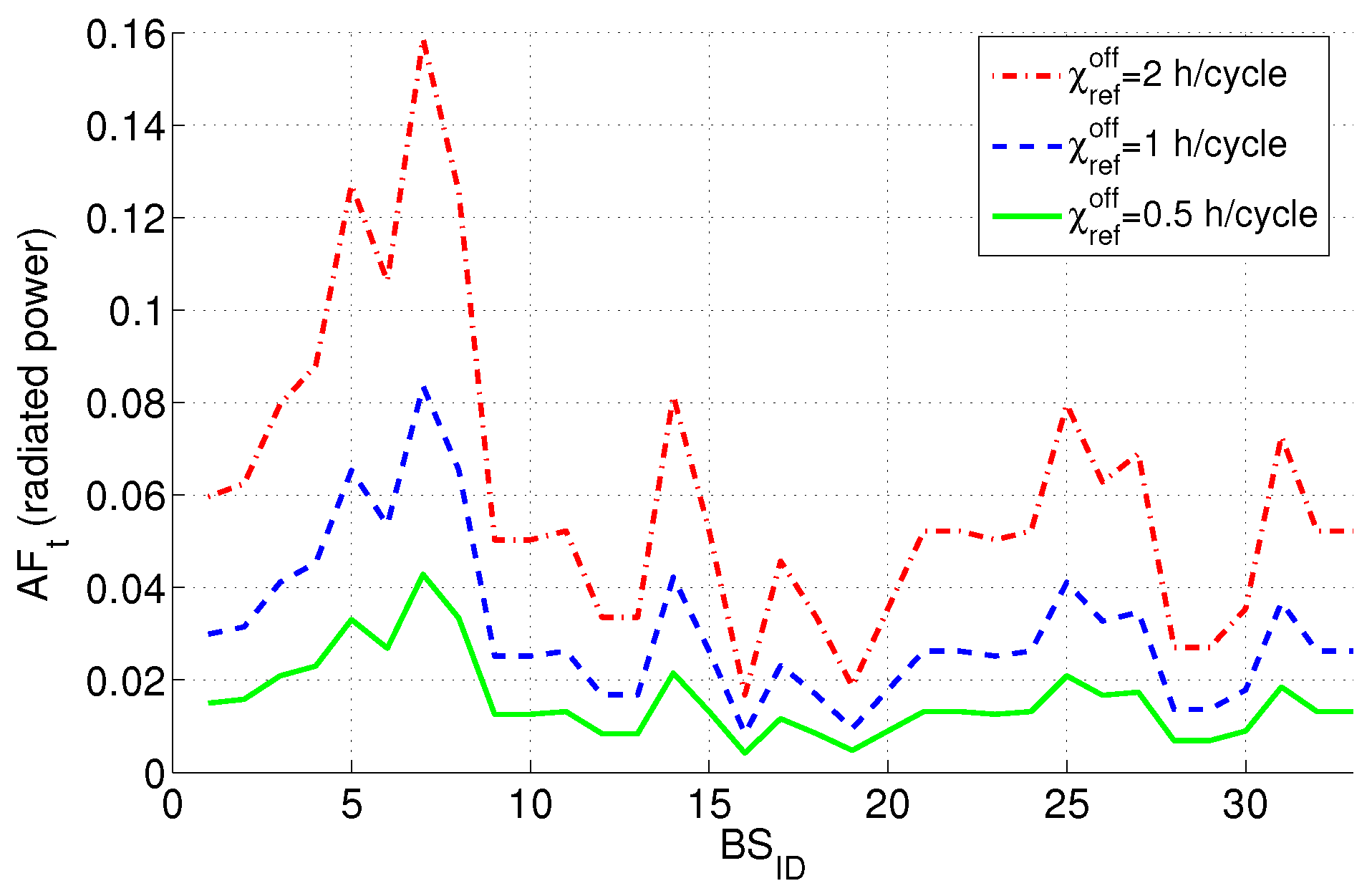
To give more insight, Figure 9 reports the term $A{F}_t$ (which depends on the radiated power) for different values of ${\chi }_{\text{ref}}^{\text{off}}$. Clearly, as the parameter ${\chi }_{\text{ref}}^{\text{off}}$ is increased, the impact on $A{F}_t$ is higher. However, the total impact of $A{F}_t$ due to radiated power is rather limited. This is due to two main reasons: (i) the power switching weight between the active states is lower compared to a power state involving SM; (ii) the highest power variation (i.e., 30 W) is seldomly applied in the scenario under consideration (see also Figure 4b).

Figure 9. $A{F}^t$ (radiated power) with the exponential model.

Figure 9. $A{F}^t$ (radiated power) with the exponential model.

6.2. Long Term Evolution Case Study Results

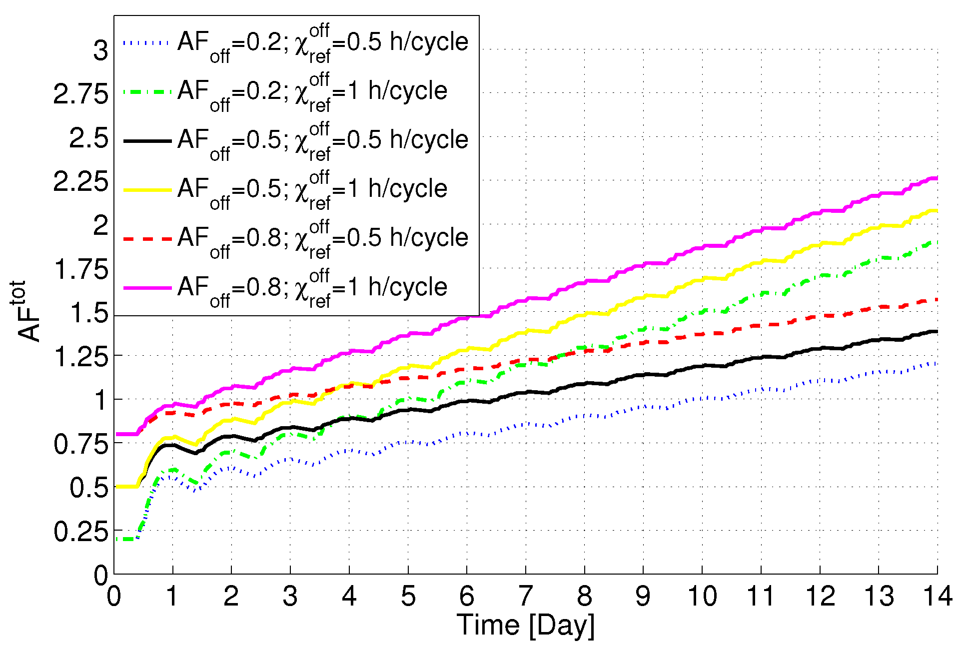
We then consider the impact on the lifetime for the LTE scenario. Unless otherwise specified, we have set a number of micro BSs equal to 10. Differently from the UMTS scenario, we take into account a time scale of 15 days. The daily traffic variation is repeated over the set of days. For each time slot we randomly place the users. We always ensure that 70% of users are placed close to the micro BSs, while 30% of users are uniformly distributed over the service area. Figure 10 reports the variation of $A{F}^{\text{tot}}$ in the network versus time for different HW parameters. In this case, the AF tends to be always increased in the network, since the micro BSs frequently change between full power and SM. 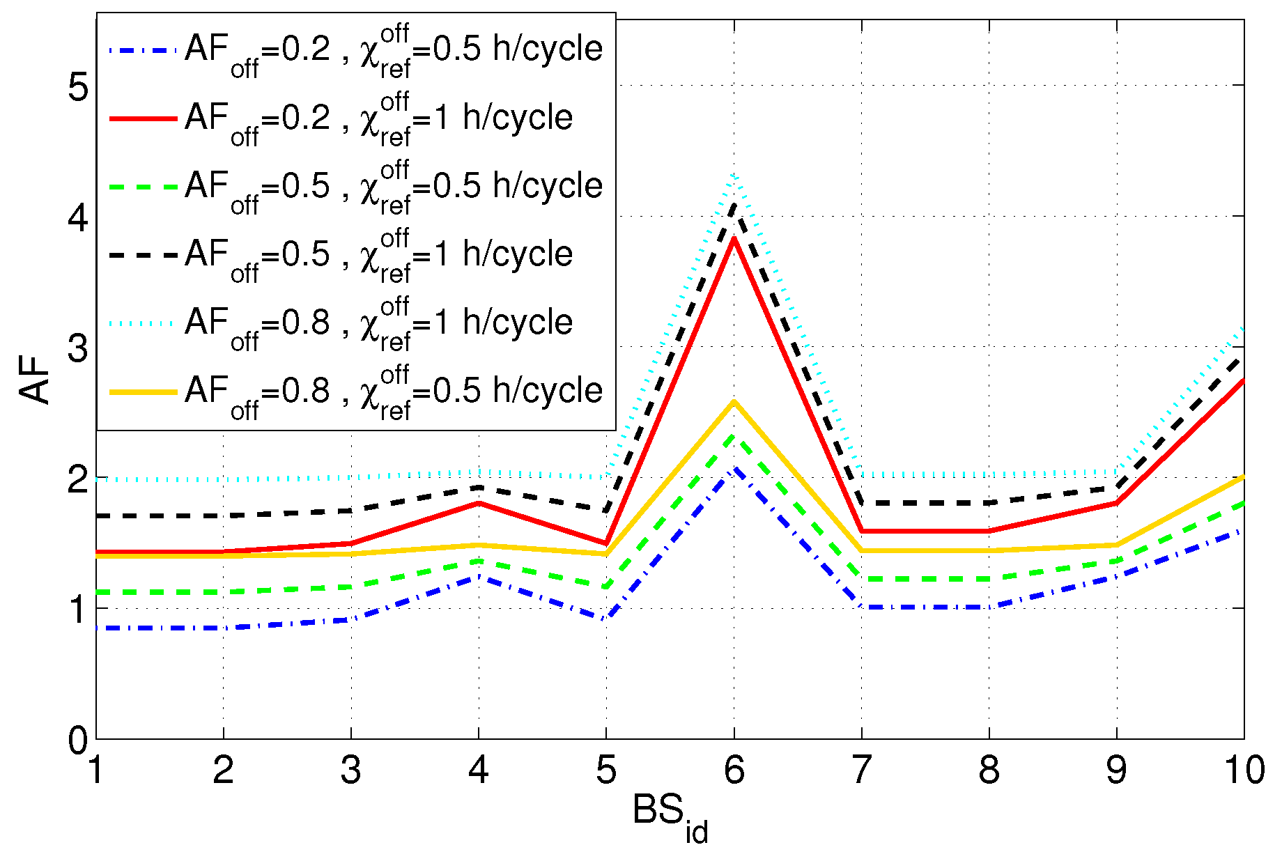As expected, the AF tends to increase when $A{F}_{\text{off}}$ is decreased and ${\chi }_{\text{ref}}^{\text{off}}$ is increased. To give more insight, Figure 11 reports the obtained AF at the end of the observation period for the different micro BSs. Also here we can clearly see that the impact on the AF is not the same for all the micro BS. For example, BS 6 experiences very frequent activations/deactivations, resulting in a lifetime reduction of a factor between two and four. On the contrary, BS 1 experiences a relatively low number of transitions, resulting in an AF always quite close to one.

Figure 10. $A{F}^{\mathrm{tot}}$ in the network vs. time for different HW parameters for the LTE scenario.

Figure 10. $A{F}^{\mathrm{tot}}$ in the network vs. time for different HW parameters for the LTE scenario.

Figure 11. AF for the single BSs for the LTE scenario.

Figure 11. AF for the single BSs for the LTE scenario.

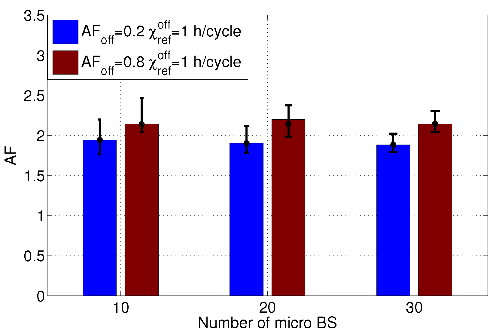
In the following, we consider the variation of the number of micro BSs in the LTE scenario in order to generalize our findings. Figure 12 reports the obtained AF for different HW parameters and a number of micro BSs varying between 10 and 30. Bars report average values, while error bars report confidence intervals (with 95% of confidence). All the results are obtained with 20 independent seeds for generating the scenario. Interestingly, we can see that the AF is influnced by the HW parameters, while the number of BSs does not consistently impact it. This is due to the fact that also the number of users grows with the number of BSs. As a result, the BSs tend to adopt a similar power scheme as $N_{\mathrm{BS}}$ is varied.

Figure 12. $A{F}^{\text{tot}}$ for different number of BSs and HW parameters.

Figure 12. $A{F}^{\text{tot}}$ for different number of BSs and HW parameters.

6.3. Cost Analysis

In the last part of our work, we consider the impact of monetary energy savings driven by energy-aware policies vs. the costs incurred from the lifetime change. In particular, we consider two distinct cases when a failure occurs on a BS: (i) a reparation can be performed (thus triggering the costs needed to pay the reparation crew); or (ii) the failed BS has to be replaced with a new one. In this analysis, we neglect the impact on users, which may bring additional costs, due to the fact a service degradation is experienced by them.

More formally, let us denote with $A{F}^{\text{tot}}\left(t\right)$ and $S\left(t\right)$ the average network AF at time t and the percentage of network power saving at time t, respectively. Moreover, D is the average equipment lifetime at full power, which we assume to be equal to 10 years in our case.

The monetary saving until time t can be expressed as:

$$\left|\mathcal{Z}\right|·{\int }_0^{t}S\left(b\right)\mathrm{d}b·P_{\text{eq}}·C_{kWh}\text{[\$]}$$

(13)

where $P_{\text{eq}}$ is the power consumption of the BS at full power, while $C_{kWh}$ is the electricity cost. (We assume in this case a time granularity equal to 1 h.)

Additionally, we compute the reparation costs at time t as:

$$\left|\mathcal{Z}\right|·\frac{A{F}^{\text{tot}}\left(t\right)}{D}·MTTR·Pers.·C_{\mathrm{m}}\text{[\$]}$$

(14)

where $MTTR$ (mean time to repair) is the average time needed to repair a BS, $Pers.$ is the number of reparation crew members, and $C_{\mathrm{m}}$ is the hourly cost for a reparation member. Note that here we have normalized $A{F}^{\text{tot}}\left(t\right)$ with D, i.e., we are translating the AF into the inverse of the actual lifetime experienced by the BS ($\frac{D}{A{F}^{\text{tot}}\left(t\right)}$).

Finally, we compute the replacement costs at time t as:

$$\left|\mathcal{Z}\right|·\frac{A{F}^{\text{tot}}\left(t\right)}{D}·C_{\text{eq}}\text{[\$]}$$

(15)

where $C_{\text{eq}}$ is the BS equipment cost. Also in this case we consider with $\frac{D}{A{F}^{\mathrm{tot}}\left(t\right)}$ the actual lifetime experienced by the BS.

The parameters used for the cost analysis are reported in Table 6. The input data come from publicly available sources. We refer the reader to [21] for more details. In brief, we focus on three key equipments: a three sector UMTS macro BS, a LTE micro Radio Resource Unit (RRU), and a LTE micro BS.

Table 6. Parameters used for the cost analysis. Mean time to repair: MTTR.

Equipment type	MTTR (h)	$\mathrm{Pers}.$	${\mathit{C}}_m$	${\text{C}}_{\mathrm{eq}}$ (USD×1000)	${\mathit{P}}_{\mathrm{eq}}$ (kW)	${\mathit{C}}_{\mathit{\text{kWh}}}$ ($)
UMTS 3 Sector Macro BS	5	2	190	32.5	1.7	0.16
LTE Micro radio resource unit (RRU)	1.5	1	190	0.65	0.05	0.16
LTE Micro BS	2	1	190	3.9	0.1	0.16

Table 6. Parameters used for the cost analysis. Mean time to repair: MTTR.

Equipment type	MTTR (h)	$\mathrm{Pers}.$	${\mathit{C}}_m$	${\text{C}}_{\mathrm{eq}}$ (USD×1000)	${\mathit{P}}_{\mathrm{eq}}$ (kW)	${\mathit{C}}_{\mathit{\text{kWh}}}$ ($)
UMTS 3 Sector Macro BS	5	2	190	32.5	1.7	0.16
LTE Micro radio resource unit (RRU)	1.5	1	190	0.65	0.05	0.16
LTE Micro BS	2	1	190	3.9	0.1	0.16

We then compute the costs/savings by considering a period of time equal to one year. In particular, we consider the UMTS scenario with 33 BSs presented in Section 5.1, and the LTE one with 10 BSs presented in Section 5.2. We then repeat the traffic profile over the whole year, and we compute the power states for each BS by applying the energy-aware algorithms. We then compute the average saving in the network $S\left(t\right)$. The saving is computed by adopting the power model presented in [29,33] for the UMTS case and LTE one, respectively. Moreover, we collect the time spent in each power state and the frequency of power transitions for each BS, and we compute the average acceleration factor in the network vs. time $A{F}^{\text{tot}}\left(t\right)$. Given $S\left(t\right)$ and $A{F}^{\text{tot}}\left(t\right)$, we then compute the savings/costs reported in Equations (13)–(15).

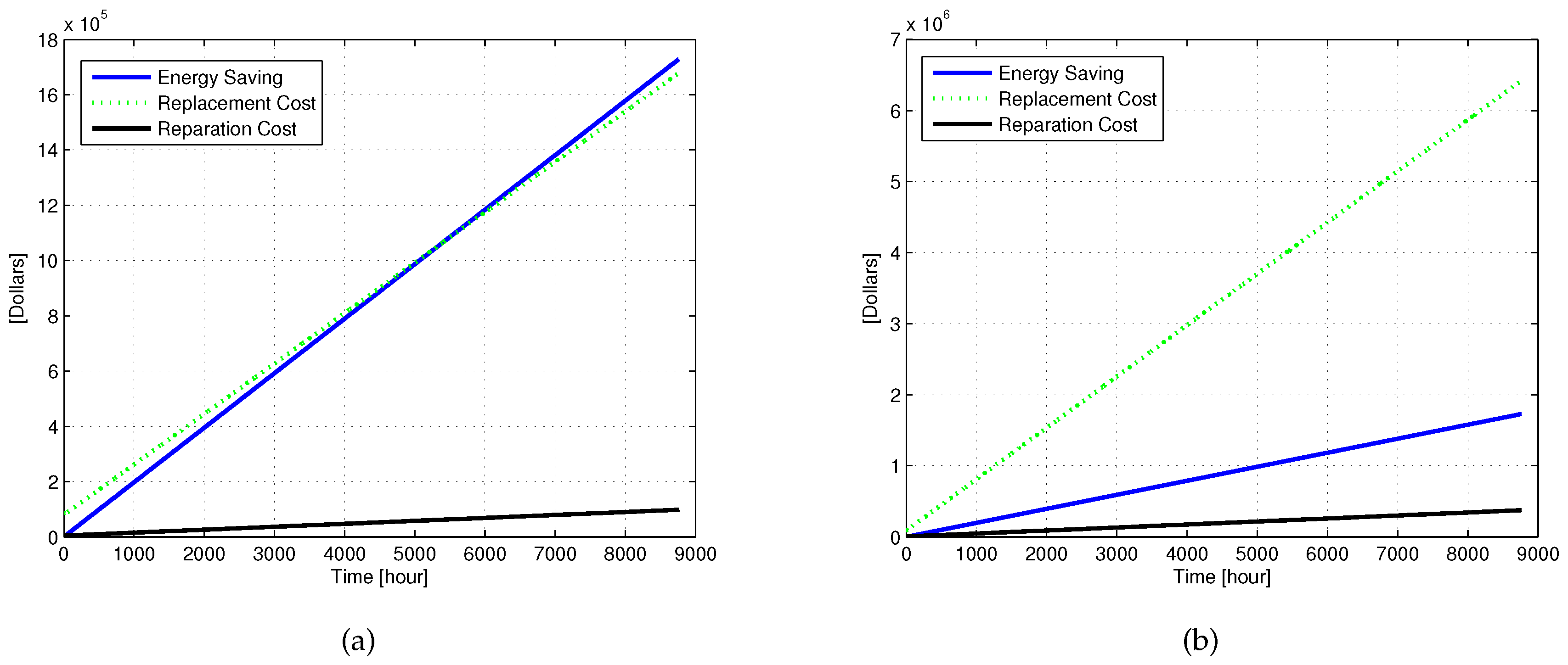
Figure 13 reports the obtained results for the UMTS case and two different HW parameters. In particular, we set $A{F}_{off}$ = 0.2, ${\chi }_{\text{ref}}^{\text{off}}$ = 0.5 (h/cycle) in one case and $A{F}_{\text{off}}$ = 0.5, ${\chi }_{\text{ref}}^{\text{off}}$ = 2 (h/cycle) in the other one. When the costs of power transitions are low (i.e., ${\chi }_{\text{ref}}^{\text{off}}$ = 0.5 (h/cycle)), the electricity energy savings are much higher compared to the reparation costs, suggesting that the gain from exploiting low power modes surpasses the increase of costs as a consequence of the lifetime decrease. However, the replacement costs are in the same order of magnitude than the savings. This suggests that, if energy-aware approaches lead to critical failures involving the device replacement, the electricity savings may be surpassed by the replacement costs. Thus, the energy-aware approaches should be carefully planned in order to integrate lifetime constraints. On the other hand, when the power transition cost increases (i.e., ${\chi }_{\text{ref}}^{\text{off}}$ = 2 (h/cycle)), the replacement costs steadily increase too, suggesting that in this case energy-aware approaches are not convenient any more for the operator.

Figure 13. Cost Analysis for the UMTS scenario. (a) $A{F}_{\text{off}}$ = 0.2, ${\chi }_{\text{ref}}^{\text{off}}$ = 0.5 h/cycle; (b) $A{F}_{\text{off}}$ = 0.5, ${\chi }_{\text{ref}}^{\text{off}}$ = 2 h/cycle.

Figure 13. Cost Analysis for the UMTS scenario. (a) $A{F}_{\text{off}}$ = 0.2, ${\chi }_{\text{ref}}^{\text{off}}$ = 0.5 h/cycle; (b) $A{F}_{\text{off}}$ = 0.5, ${\chi }_{\text{ref}}^{\text{off}}$ = 2 h/cycle.

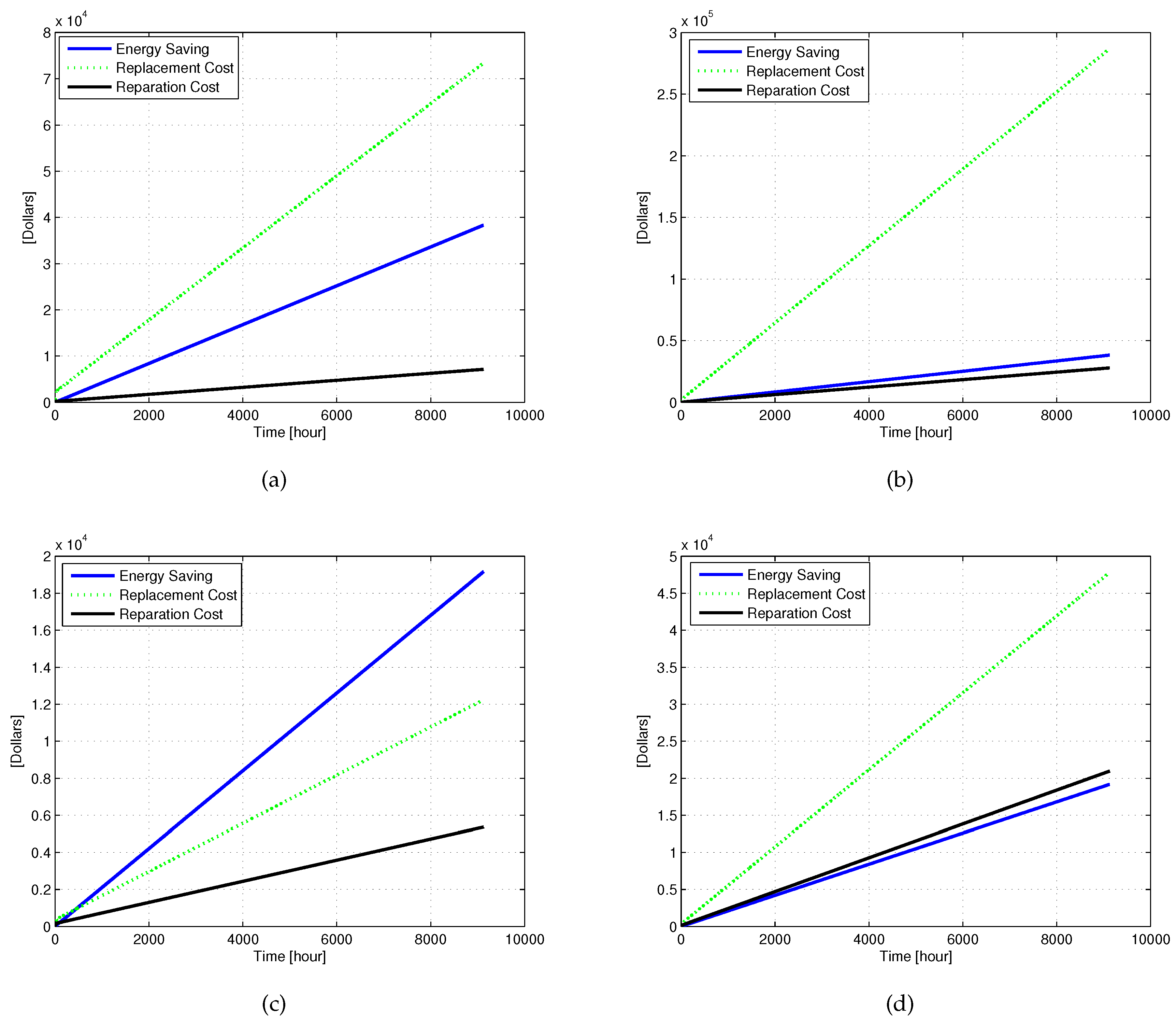
In the following, we consider the LTE scenario with 10 micro, and a period of time equal to one year. Figure 14 reports the results for this scenario. In particular, we consider two possible targeted devices (i.e., a micro LTE RRU and a micro LTE BS), and two settings for the HW parameters (like in the UMTS case). Focusing on the micro BS results (reported in Figure 14a,b) we can clearly see that the replacement costs are always higher than the electricity savings. On the contrary, the reparation costs are lower. Thus, the savings may be higher of lower than the costs. This suggests again the importance of a careful management of the energy-aware approaches, in order to limit the impact on the costs due to the lifetime decrease. Finally, Figure 14c,d report the results for the LTE RRU case. Interestingly, in this case the electricity savings always compensate the lifetime reduction costs when the power transition cost is low (i.e., ${\chi }_{\text{ref}}^{\text{off}}$ = 0.5 (h/cycle)). On the contrary, when the power transition cost is equal to 2 (h/cycle) both the replacement and the reparation costs are always higher than the savings, suggesting that also the design of the device (and consequently its HW parameters) plays a crucial role in determining the effectiveness of energy-aware approaches.

7. Discussion

The presented results show that it is of mandatory importance to develop solutions to limit the impact of power states parameters on the lifetime. Note that this approach is completely new and different from previous solutions (like e.g., [18]) which focus on the limitation of the number of power switching transitions throughout the day. More in depth, limiting the number of power switching transitions per day may not be the best choice for the lifetime, since the lifetime requires a longer time scale. In particular, the lifetime model is not considered in previous works. This fact then brings to two negative effects. First, the lifetime increase as a consequence of the adoption of low power states is not taken into account. Second, the number of transitions should not be the same over time. When the device is new, it may change the power state more frequently. However, when different power changes are applied, the number of new transitions has to be reduced, as a consequence of the lifetime decrease. The effects of power state transitions (both positive and negative) are considered in our work. We believe that our model can be applied for the definition of new algorithms for the maximization of the lifetime in cellular networks.

Figure 14. Cost Analysis for the LTE scenario. (a) LTE Micro BS-$A{F}_{\text{off}}$ = 0.2, ${\chi }_{\text{ref}}^{\text{off}}$ = 0.5 h/cycle; (b) LTE Micro BS-$A{F}_{\text{off}}$ = 0.5, ${\chi }_{\text{ref}}^{\text{off}}$ = 2 h/cycle; (c) LTE RRU Micro-$A{F}_{\text{off}}$ = 0.2, ${\chi }_{\text{ref}}^{\text{off}}$ = 0.5 h/cycle; (d) LTE RRU Micro-$A{F}_{\text{off}}$ = 0.5, ${\chi }_{\text{ref}}^{\text{off}}$ = 2 h/cycle.

Figure 14. Cost Analysis for the LTE scenario. (a) LTE Micro BS-$A{F}_{\text{off}}$ = 0.2, ${\chi }_{\text{ref}}^{\text{off}}$ = 0.5 h/cycle; (b) LTE Micro BS-$A{F}_{\text{off}}$ = 0.5, ${\chi }_{\text{ref}}^{\text{off}}$ = 2 h/cycle; (c) LTE RRU Micro-$A{F}_{\text{off}}$ = 0.2, ${\chi }_{\text{ref}}^{\text{off}}$ = 0.5 h/cycle; (d) LTE RRU Micro-$A{F}_{\text{off}}$ = 0.5, ${\chi }_{\text{ref}}^{\text{off}}$ = 2 h/cycle.

Additionally, we have shown that the lifetime is also influenced by HW parameters, which instead depend on the components used to build the device. Since mesurements of these parameters are not yet available in the literature, we have performed a sensitivity analysis on them. However, we stress the importance of precisely estimating these parameters in a cellular network. We believe that this task can be an interesting direction for future work. In particular, measurements of temperature vs. power consumption of a BS in operation would ease the setting of the HW parameters presented in this paper. In addition, the validation of the presented failure rate models in a real cellular deployment is another open issue. This activity can then lead to the definition of new failure rate models, more tailored to cellular networks. Finally, our model is applied to the whole BS. However, the impact on lifetime on the single components should be also investigated, i.e., to assess how much each component is critical for the BS lifetime.

8. Conclusions and Future Work

We have presented a model to evaluate the lifetime of a BS taking into account the different power states and the transitions between one state and another one. The model integrates both HW parameters and power state transitions parameters, that depend on the policy used to change the device power. We have proposed both a linear model and an exponential model for the HW parameters. We have then evaluated the lifetime increase/decrease compared to a reference lifetime by means of the AF, a metric that is inversely proportional to the lifetime. Finally, we have evaluated the model on different scenarios (based on UMTS and LTE technologies), and different BS types (e.g., micro, macro, RRU). Our results indicate that the lifetime may be negatively impacted when frequent power state transitions take place. In particular, the largest lifetime decrease is experienced when the BS passes from SM to an active state (and vice-versa). Moreover, we have shown that the lifetime varies over a set of BSs, with some BSs increasing it and other showing a lifetime decrease. Additionally, we have shown that the lifetime varies over time, and that the reparation/replacement costs influenced by the lifetime decrease may even surpass the electricity saved by reducing energy. All these facts suggest that the impact of lifetime should be carefully considered when power state transitions (especially the ones involving SMs) are planned. As future work, we plan to propose new algorithms that integrate lifetime, energy consumption and user constraints in order to decide when and how to change the power state for each BS in the network. Moreover, we plan to perform lifetime measurements on real devices considering different BS types, different BS technologies, and different failure types (e.g., triggered by HW failures and/or software ones). Finally, we plan to apply our model also to future cloud radio access networks (C-RANs) [34].