Optimal Operation of Combined Heat and Power System Based on Forecasted Energy Prices in Real-Time Markets

Abstract

This paper develops a discrete operation optimization model for combined heat and powers (CHPs) in deregulated energy markets to maximize owners’ profits, where energy price forecasting is included. First, a single input and multi-output (SIMO) model for typical CHPs is established, considering the varying ratio between heat and electricity outputs at different loading levels. Then, the energy prices are forecasted with a gray forecasting model and revised in real-time based on the actual prices by using the least squares method. At last, a discrete optimization model and corresponding dynamic programming algorithm are developed to design the optimal operation strategies for CHPs in real-time. Based on the forecasted prices, the potential operating strategy which may produce the maximum profits is pre-developed. Dynamic modification is then conducted to adjust the pre-developed operating strategy after the actual prices are known. The proposed method is implemented on a 1 MW CHP on a typical day. Results show the optimized profits comply well with those derived from real-time prices after considering dynamic modification process.

1. Introduction

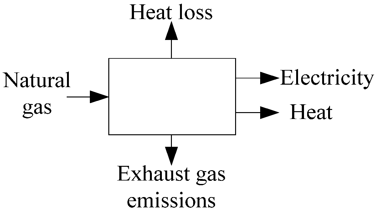
The combined heat and power (CHP) system produces heat and electricity with high efficiency by consuming oil, natural gas, and biomass, etc. [1]. The well-known cogeneration system has been considered to be the most promising alternative to traditional energy supplying systems. Compared to conventional generation of heat and electricity in a decoupled way, the overall efficiency of the co-generating technique can reach up to 70%–80% [2,3]. As a low-carbon, cost-effective, and high energy conversion efficiency technology, the total capacity of CHP is expected to reach 483.7 GW in 2023 worldwide [4].

Generally, CHPs’ operating strategies are categorized into two groups: heat lead (HL) and electricity lead (EL) [5]. For HL CHPs, they are operated mainly to satisfy heat load and the heat deficit is imported from auxiliary boilers, district heating or heating grid [6]. While for EL CHPs, electric loads are satisfied first and the deficient demand is provided from the power grid. The main drawback for the two types of CHPs is the inflexibility between electric and heat output. Heat to power ratio (HTPR) is introduced to characterize the heat and electric output proportion, which is also closely linked with overall efficiency and loading level of CHPs [7,8]. Thus, CHPs can be operated at different loading levels to serve various heat and electric loads.

The existing literatures on CHP operation mainly concentrate on achieving economic goals (e.g., low operation cost, reduction of fuel consumption) and environmental goals (e.g., low carbon dioxide emission). The output of CHP is optimized to minimize the annual operating and maintaining costs of the whole system in [9]. The heat and electric loads are supposed to be known, which might lead to inaccuracy if actual demand diverts greatly from the forecasted demand. The least-cost operating strategy for CHPs is studied in [10], and results show that the strategy does not mean the lowest carbon dioxide emission. Thus in [11], the optimal strategy for CHPs is studied by taking several indicators into account, including the least energy consumption, the lowest operation cost and the lowest carbon dioxide emission. The main disadvantage of the mentioned literatures is that energy prices are supposed to be constant for a long period of time. As a result, the CHPs are not optimized in real-time, failing to reflect the actual conditions.

In order to address the problem, various optimization algorithms have been proposed to achieve real-time energy management. A comprehensive review of modeling methods, planning approaches (various indicators are introduced) and energy management algorithms for a combined cooling, heat, and power (CCHP) microgrid are presented in [12]. An online algorithm is devised in [13] for real-time energy management. The algorithm is superior to conventional dynamic programming approaches in realization of arbitrary energy prediction errors. An optimal power management strategy for hybrid energy systems is presented in [14], aiming to minimize the total cost and fuel emissions. In [15], the optimal size of a CHP-plant with thermal store is analyzed in the Germany spot market to maximize the profits, where only the electricity spot price is considered and the other prices (those of heat and gas) are supposed to be constant. In [16], a CHP-based district heating system with renewable energy source and energy storage system is optimized by using LP (linear programming) method, where the overall costs of net heat and power acquisition is minimized effectively. A model predictive control strategy is proposed for the CHP to achieve effective demand response in [17]. The results show the cost reductions for the households reach their highest when the real-time energy prices fluctuate strongly. Reference [18] proposes a smart hybrid renewable energy for communities (SHREC) system, where both thermal and electricity markets are considered. A planning model is developed for the SHREC system and optimized by using the LP algorithm, whose effectiveness and flexibility are verified through specific calculation results.

All the aforementioned literatures proposed effective approaches to design optimal operating strategy for the CHP from different aspects. While during the research, the real-time energy prices are assumed to have been already known. However, in real-time markets, the prices of electricity, heat, and natural gas are not known in advance. The operation schedules of CHPs are pre-developed based on forecasted prices or load conditions. On the other hand, the influence of loading level on overall efficiency and HTPR of CHPs is not considered either. The overall efficiency is generally in positive correlation with the loading level of CHPs, i.e., a high loading level means high overall efficiency. Another problem for existing researches is that the profit optimization of CHP considering the forecast prices is neglected, where the profits of pre-developed operating strategy differ greatly from those of adjusted strategy in response to actual prices. In deregulation energy markets, the profits are key incentive for CHP owners. Thus, to optimize the profits of CHPs in real-time, there are several challenges: (i) to determine the heat and electricity output proportion, i.e., HTPR; (ii) to forecast energy prices; (iii) to adjust pre-developed operating strategies to comply with actual conditions.

A discrete operation optimization model is developed in this paper to devise the optimal operation strategy for CHPs in real-time, where the profits reach the maximum. First, the SIMO (single input and multi-output) CHP model is established, where both the overall efficiency and HTPR are in variation with the loading level. Then, energy prices, including that of heat, electricity and natural gas, are forecasted by the gray forecasting model GM(1,n) (i.e., first-order, n variables grey model) and revised with actual prices by using the least square method. Finally, a discrete optimization model is developed to obtain the optimal operating points, which may produce maximum profits. The profits are optimized every 30 min, which determine the heat and electricity output in real-time. Then the operating strategy is pre-developed based on the forecasted prices. A dynamic programming algorithm is proposed to adjust the pre-developed strategy after actual prices are known, where the maximum profits are achieved through reducing the profit loss during the modification to the least. The proposed model and optimization approach are demonstrated with a 1MW CHP under different loading levels.

The novelty of this paper is that it: (i) introduces varying HTPR with respect to the loading level of CHP, which is fixed in most previous research; (ii) proposes a discrete optimization model to project the indication optimal operating points which may produce potential maximum profits; (iii) proposes a dynamic programming algorithm to obtain the maximum profits based on actual and forecasted energy prices.

The remaining parts of this paper are organized as follows. In Section 2, the SIMO model for CHP is established, whose overall efficiency and HTPR both vary with the loading level. The price forecasting method is presented in Section 3. Then the discrete optimization model for CHP is developed in Section 4, followed by the dynamic programming algorithm. In Section 5, a 1 MW CHP is optimized with the proposed approach. Finally, conclusions are drawn in Section 6.

2. Modeling of Combined Heat and Power

2.1. Basic Diagram of Combined Heat and Power

The main characteristic of CHPs is that they reuse waste heat from prime mover during electricity generation processes to serve thermal loads, which is superior to traditional boilers. Extraction-condensing steam turbine-based CHP is very popular because the ratio between heat and electricity output could be adjusted according to various loading ratios between the two loads, providing more flexibility during peak and off-peak hours [19].

A typical CHP system consists of a combustion chamber, a turbine generator and a heat recovery boiler according to [20]. The SIMO model of CHP can then be established, shown in Figure 1.

In the SIMO model of CHP, two key parameters should be determined first: overall energy conversion efficiency and HTPR.

Figure 1. Single input and multi-output (SIMO) model of combined heat and power (CHP).

Figure 1. Single input and multi-output (SIMO) model of combined heat and power (CHP).

2.2. Key Parameters of Combined Heat and Power

2.2.1. Overall Energy Conversion Efficiency

As shown in Figure 1, the output of a CHP system mainly includes four parts: electricity, heat, and unavoidable heat loss and exhaust gas emissions, while only the heat and electricity output are called useful energy. The overall energy conversion efficiency of a CHP is expressed as:

$$\mathsf{\eta }=\frac{Q_{\mathrm{\Sigma }}}{G}$$

(1)

where η is the overall efficiency; Q_Σ is the useful energy converted from natural gas, which is also the total energy of heat and electricity, in kJ; G is the energy of natural gas, in kJ.

In most existing research, the nominal value of η is adopted. However, η is found to be changing with different loading levels and operating modes of CHPs [21]. The overall efficiency is mainly determined and affected by the loading level and generally, expressed as:

$$\mathsf{\eta }=\text{f}\left(L\right)$$

(2)

where L is CHP’s loading condition.

A typical curve of η is shown in Figure 2, which is derived from [22]. When the CHP’s loading is lower than L₁, η is zero, indicating that it is not economic to run the CHP because the cost is higher than its income. When the CHP is fully loaded, η reaches its nominal value, denoted by η_N (about 90%). As shown in Figure 2, the curve of η is divided into five sections. At low loading level, η increases more rapidly than that at high loading level.

Figure 2. Relation between η and loading level.

Figure 2. Relation between η and loading level.

In Figure 2, η₁, η₂, η₃, and η₄ are the overall efficiency of CHP in response to loading level: L₁, L₂, L₃, and L₄ respectively, which can be modeled as a discrete function:

$$\mathsf{\eta }=\{\begin{array}{llllll}{\text{f}}_1\left(L\right)=0\hfill & & & & & 0\le L<L_1\hfill \\ {\text{f}}_2\left(L\right)\hfill & & & & & L_1\le L<L_2\hfill \\ {\text{f}}_3\left(L\right)\hfill & & & & & L_2\le L<L_3\hfill \\ {\text{f}}_4\left(L\right)\hfill & & & & & L_3\le L<L_4\hfill \\ {\text{f}}_5\left(L\right)\hfill & & & & & L_4\le L<L_N\hfill \end{array}$$

(3)

The field test is usually conducted by the manufacturers to obtain the efficiency data under different loading levels. The η-load curve of a CHP is then got through curve fitting.

2.2.2. Heat to Power Ratio

Although CHPs are able to provide heat and electricity simultaneously, there is a fixed relation between the two products. To study the ratio between heat and electricity, ${\mathsf{\gamma }}_{\text{E}}$ and ${\mathsf{\gamma }}_{\text{H}}$, are introduced.

$$\{\begin{array}{c}{E}_{\text{CHP}}={\mathsf{\gamma }}_E{Q}_{\mathrm{\Sigma }}\\ H_{\text{CHP}}={\mathsf{\gamma }}_H{Q}_{\mathrm{\Sigma }}\end{array}$$

(4)

where $E_{\text{CHP}}$ is the energy of electricity generated by CHP, in kJ; $H_{\text{CHP}}$ is the energy of heat generated by CHP, in kJ; ${\mathsf{\gamma }}_{\text{E}}$ and ${\mathsf{\gamma }}_{\text{H}}$ are just used to describe the energy proportion of $E_{\text{CHP}}$ and $H_{\text{CHP}}$, respectively, and there is no practical significance for them.

By substituting Equation (1) into Equation (4), the output of CHP can be expressed in another form:

$$\{\begin{array}{c}{E}_{\text{CHP}}={\mathsf{\gamma }}_{\text{E}}\mathsf{\eta }G\\ H_{\text{CHP}}={\mathsf{\gamma }}_{\text{H}}\mathsf{\eta }G\end{array}$$

(5)

where ${\mathsf{\gamma }}_{\text{E}}\mathsf{\eta }$ is usually called electric efficiency of CHP, also denoted by ${\mathsf{\eta }}_{\text{E}}$; ${\mathsf{\gamma }}_{\text{H}}\mathsf{\eta }$ is usually called the heat efficiency of CHP, also denoted by ${\mathsf{\eta }}_{\text{H}}$.

Apparently, ${\mathsf{\gamma }}_{\text{E}}$ and ${\mathsf{\gamma }}_{\text{H}}$ naturally satisfy:

$${\mathsf{\gamma }}_{\text{H}}+{\mathsf{\gamma }}_{\text{E}}=1$$

(6)

The HTPR of CHPs is defined as the ratio of the heat output to the electricity output, which reflects the ability of CHPs to meet heat and electric demand. The HTPR of CHPs, denoted by $\mathsf{\zeta }$, is expressed as:

$$\mathsf{\zeta }=\frac{H_{\text{CHP}}}{E_{\text{CHP}}}=\frac{{\mathsf{\gamma }}_{\text{H}}}{{\mathsf{\gamma }}_{\text{E}}}$$

(7)

According to [23], the loading level will influence the HTPR, but the specific relation between them is not addressed. Based on the research in [24,25], the $\mathsf{\zeta }$-load curve should be a step function with several intervals. A typical $\mathsf{\zeta }$-loading level curve is shown in Figure 3.

Figure 3. Relation between $\mathsf{\zeta }$ and loading level.

Figure 3. Relation between $\mathsf{\zeta }$ and loading level.

From Figure 3, the step function for $\mathsf{\zeta }$ can be expressed as:

$$\mathsf{\zeta }=\{\begin{array}{llllll}{\mathsf{\zeta }}_1=0\hfill & & & & & 0\le L<L_1^{\prime }\hfill \\ {\mathsf{\zeta }}_2\hfill & & & & & L_1^{\prime }\le L<L_2^{\prime }\hfill \\ {\mathsf{\zeta }}_3\hfill & & & & & L_2^{\prime }\le L<L_3^{\prime }\hfill \\ {\mathsf{\zeta }}_4\hfill & & & & & L_3^{\prime }\le L<L_4^{\prime }\hfill \\ {\mathsf{\zeta }}_5\hfill & & & & & L_4^{\prime }\le L<L_N\hfill \end{array}$$

(8)

In Figure 3, there are five sections for the $\mathsf{\zeta }$-load curve: including four non-zero sections and a zero section. When the loading level is less than $L_1^{\prime }$, the CHP does not work, and the HTPR is zero, correspondingly. The higher the loading level is, the lower the HTPR will be. At low loading level, the heat efficiency is higher than electricity efficiency. At high loading level, the overall efficiency of CHP increases a lot, and the electricity efficiency increases correspondingly. More generally, the relation between ζ and the overall efficiency of CHP is also studied in [26]. If the efficiency reaches certain threshold, the CHP will then be operated at a new HTPR.

3. Price Forecasting

When optimizing the operation strategy of CHPs to achieve maximum profits, energy prices should also be determined. In the wholesale market, electric price varies at 30-min resolution. The real-time price of natural gas and heat are supposed to be varying every 30 min as well in the study. Each price interval is also called a dispatching step and therefore there are 48 dispatching steps in one day. Usually, the real-time prices of the kth dispatching step are not known until beforehand. Thus, the operation schedules of CHPs should be pre-determined based on forecasted prices. The real-time energy prices fluctuate with the load of the energy system, the climate and so on. However, there is still strong regularity compared to the history prices for the same time in one day.

For the energy prices are relevant to several factors, the gray forecasting model GM(1,n) [27] is adopted in this paper to forecast the energy prices. In the model, “1” means the first-order differential equations are used and “n” is the number of relevant variables. Suppose the price to be forecasted at $t$ is $x_1$, and the historical price series is $X_1^0=\left(x_1^0\left(1\right),x_1^0\left(2\right),\cdots ,x_1^0\left(m\right),\cdots x_1^0\left(M\right)\right)$, where $x_1^0\left(i\right)$ is the historical price for different days at $t$. The relevant variable (including load, climate and etc.) sequences are:

$$\{\begin{array}{c}{X}_2^0=\left(x_2^0\left(1\right),x_2^0\left(2\right),\cdots ,x_2^0\left(m\right),\cdots x_2^0\left(M\right)\right)\\ X_3^0=\left(x_3^0\left(1\right),x_3^0\left(2\right),\cdots ,x_3^0\left(m\right),\cdots x_3^0\left(M\right)\right)\\ ⋮\\ X_n^0=\left(x_n^0\left(1\right),x_n^0\left(2\right),\cdots ,x_n^0\left(m\right),\cdots x_n^0\left(M\right)\right)\end{array}$$

(9)

where $X_i^0,i=2,3,\cdots ,n$ is the historical value series for the ith variable in M days at the fixed time t; $x_i^0\left(m\right)$ is historical value of the ith variable in the mth day.

Then calculate the 1-AGO (accumulated generating operation) sequence for each relevant variable to reduce the randomness of the data:

$$X_i^{\left(1\right)}=\left\{x_i^{\left(1\right)}\left(1\right),x_i^{\left(1\right)}\left(2\right),\cdots x_i^{\left(1\right)}\left(m\right),\cdots x_i^{\left(1\right)}\left(M\right)\right\}$$

(10)

where $i=2,3,\cdots ,n$ and $x_i^{\left(1\right)}\left(k\right)={\displaystyle \sum _{j=1}^k{x}_i^0\left(j\right)}$, $k=1,2,\cdots ,M$.

The adjacent mean value sequence for $X_i^{\left(1\right)}$ is calculated as follows:

$$Z_i^{\left(1\right)}=\left\{z_i^{\left(1\right)}\left(1\right),z_i^{\left(1\right)}\left(2\right),\cdots z_i^{\left(1\right)}\left(m\right),\cdots z_i^{\left(1\right)}\left(M-1\right)\right\}$$

(11)

where $i=2,3,\cdots ,n$ and $z_i^{\left(1\right)}\left(k\right)=\frac{1}{2}\left(x_i^{\left(1\right)}\left(k\right)+x_i^{\left(1\right)}\left(k+1\right)\right)$, k = 1, 2, …, M − 1.

Based on $X_i^{\left(1\right)}$ and $Z_i^{\left(1\right)}$, $x_1$ is obtained with the $GM\left(1,n\right)$ model. The forecasting method mentioned above is applied in each dispatching step to get the forecasted prices for heat, electricity, and natural gas in one day.

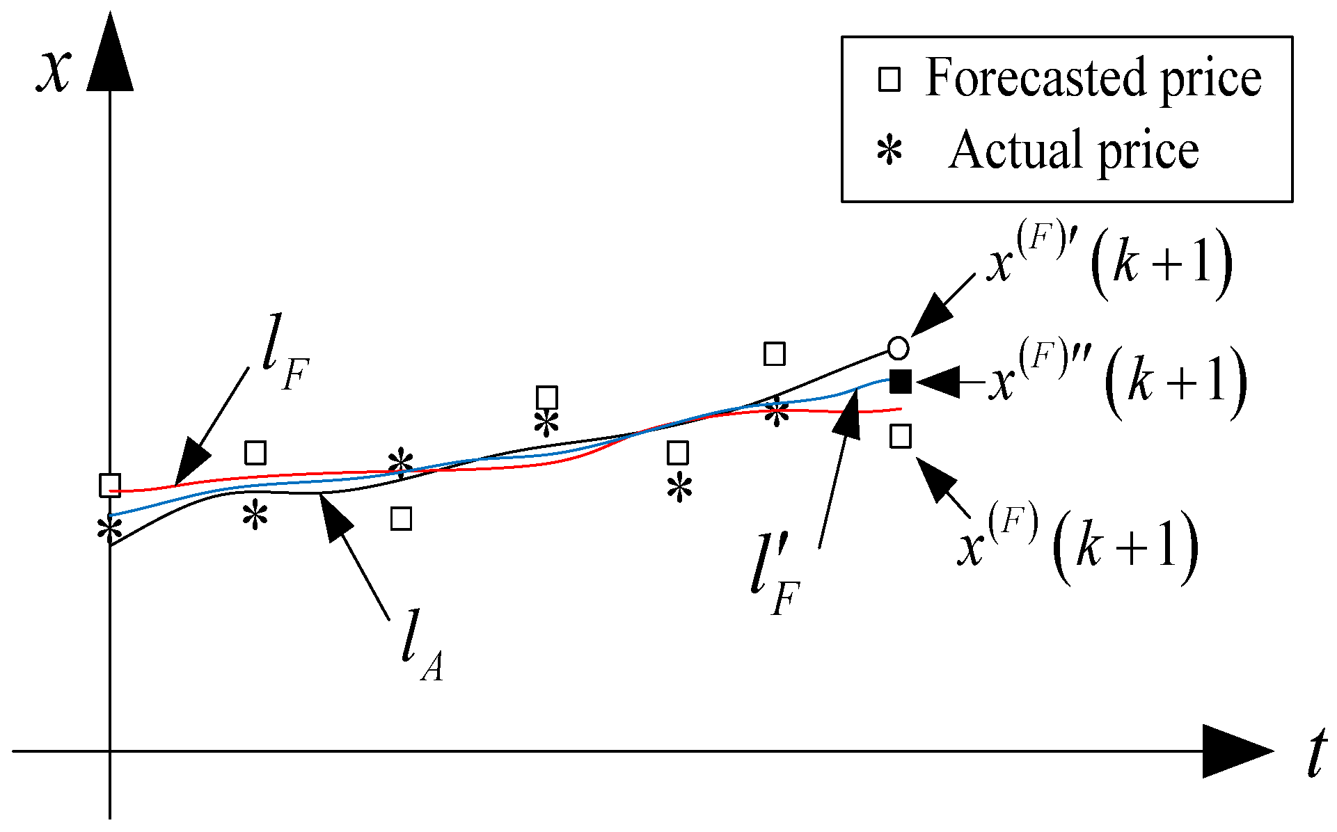
After the actual prices for heat, electricity, and natural gas are known at the start of kth dispatching step, the forecasted prices for the (k + 1)th dispatching step should be revised with certain method. Suppose the forecast prices for k + 1 dispatching steps are $X^{\left(\text{F}\right)}=(x^{\left(\text{F}\right)}\left(1\right),x^{\left(\text{F}\right)}\left(2\right),x^{\left(\text{F}\right)}\left(3\right),\cdots ,$ $x^{\left(\text{F}\right)}\left(k+1\right))$, which are obtained from the gray forecasting model, and the actual prices for k dispatching steps are $X^{\left(\text{A}\right)}=\left(x^{\left(\text{A}\right)}\left(1\right),x^{\left(\text{A}\right)}\left(2\right),x^{\left(\text{A}\right)}\left(3\right),\cdots ,x^{\left(\text{A}\right)}\left(k\right)\right)$. The fitting price curves for $X^{\left(\text{F}\right)}$ and $X^{\left(\text{A}\right)}$ can then be obtained by using the least squares method, as shown in Figure 4.

Figure 4. Fitting price curves.

Figure 4. Fitting price curves.

In Figure 4, $l_{\text{A}}$ is the fitting curve for $X^{\left(\text{A}\right)}$ and a new forecasted price $x^{{\left(\text{F}\right)}^{\prime }}\left(k+1\right)$ (denoted by a small circle) for the (k + 1)th dispatching step is obtained. $l_F$ in red is the fitting curve for $X^{\left(\text{F}\right)}$. The blue curve $l_{\text{F}}^{\prime }$ is obtained by using the least square method, whose square of distance to $l_{\text{A}}$ and $l_{\text{F}}$ is the minimum. At last, the revised forecasted price $x^{{\left(\text{F}\right)}^{″}}\left(k+1\right)$ (denoted by a small solid square) is obtained, which is in the curve $l_{\text{F}}^{\prime }$.

4. Operation Optimization of Combined Heat and Power

4.1. Discrete Optimization Model for Combined Heat and Power

In the wholesale market, electricity, heat and natural gas prices all vary at 30-min resolution, denoted by $p_{\text{E}}$, $p_{\text{H}}$ and $p_{\text{G}}$, respectively. Thus, CHPs could be operated according to the combination of the three prices to maximize benefits in the 48 dispatching steps.

In the $k\mathrm{t}\mathrm{h}$ dispatching step, the profit is calculated by:

$${\text{PRO}}_{\text{CHP}}\left(k\right)=I_{\text{H}}(k)+I_{\text{E}}(k)-C_{\text{G}}(k)$$

(12)

where PRO is abbreviation of profit and ${\text{PRO}}_{\text{CHP}}\left(k\right)$ denotes the profit in the kth step; $I_{\text{H}}(k)$ and $I_{\text{E}}(k)$ are the income from selling heat and electricity, respectively; $C_{\text{G}}(k)$ is the cost of buying natural gas.

Equation (12) can be further written as follows:

$${\text{PRO}}_{\text{CHP}}\left(k\right)=H_{\text{CHP}}\left(k\right)p_{\text{H}}\left(k\right)+E_{\text{CHP}}\left(k\right)p_{\text{E}}\left(k\right)-V_{\text{G}}\left(k\right)p_{\text{G}}\left(k\right)$$

(13)

where $V_{\text{G}}(k)$ is the volume of natural gas consumed in the $k\mathrm{t}\mathrm{h}$ dispatching step; $p_{\text{H}}\left(k\right)$, $p_{\text{E}}\left(k\right)$ and $p_{\text{G}}\left(k\right)$ are the prices of heat, electricity and natural gas in the $k\mathrm{t}\mathrm{h}$ dispatching step respectively.

Usually, the energy contained in a cubic meter of natural gas is a constant, denoted by $q$, in kJ/m³. Thus the total energy injected into the CHP in the $k\mathrm{t}\mathrm{h}$ step is expressed as:

$$G\left(k\right)=q{V}_{\text{G}}\left(k\right)$$

(14)

Through substituting Equation (6) into Equation (7), ${\mathsf{\gamma }}_H$ and ${\mathsf{\gamma }}_E$ are obtained and shown as follows:

$$\{\begin{array}{c}{\mathsf{\gamma }}_H=\frac{\mathsf{\zeta }}{1+\mathsf{\zeta }}\\ {\mathsf{\gamma }}_E=\frac{1}{1+\mathsf{\zeta }}\end{array}$$

(15)

By substituting Equations (5), (14) and (15) into Equation (13), the objective function of CHP is obtained, given by:

$$\begin{array}{c}\text{Maximize: }{\text{PRO}}_{\text{CHP}}\left(k\right)\\ {\text{PRO}}_{\text{CHP}}\left(k\right)=\left(\frac{\mathsf{\zeta }}{1+\mathsf{\zeta }}q\mathsf{\eta }{p}_{\text{H}}\left(k\right)+\frac{1}{1+\mathsf{\zeta }}q\mathsf{\eta }{p}_{\text{E}}\left(k\right)-p_{\text{G}}\left(k\right)\right)V_{\text{G}}\left(k\right)\end{array}$$

(16)

To solve the objective function Equation (16), we define a new variable ${\text{PRO}}_{\text{CHP\_base}}\left(k\right)$, which means the profit obtained through consuming a cubic meter of natural gas by CHP:

$${\text{PRO}}_{\text{CHP\_base}}\left(k\right)=\frac{\mathsf{\zeta }}{1+\mathsf{\zeta }}q\mathsf{\eta }{p}_{\text{H}}\left(k\right)+\frac{1}{1+\mathsf{\zeta }}q\mathsf{\eta }{p}_{\text{E}}\left(k\right)-p_{\text{G}}\left(k\right)$$

(17)

Obviously, as long as ${\text{PRO}}_{\text{CHP\_base}}\left(k\right)$ reaches its maximum, the maximum value of ${\text{PRO}}_{\text{CHP}}\left(k\right)$ will be obtained. In Equation (17), after $\mathsf{\zeta }$, $p_{\mathrm{H}}\left(k\right)$, $p_{\text{E}}\left(k\right)$, and $p_{\text{G}}\left(k\right)$ are all determined in the $k\mathrm{t}\mathrm{h}$ dispatching step, ${\text{PRO}}_{\text{CHP}}\left(k\right)$ is just a function of η, which is quite easy to solve.

There are also a set of constraints which must be satisfied during optimization.

4.1.1. Output Constraints

The heat and electricity outputs of CHP must vary between their maximum and minimum capacities, respectively:

$$\{\begin{array}{c}{H}_{\text{CHP,min}}\le H_{\text{CHP}}\left(k\right)\le H_{\text{CHP,max}}\\ E_{\text{CHP,min}}\le E_{\text{CHP}}\left(k\right)\le E_{\text{CHP,max}}\end{array}$$

(18)

where $H_{\text{CHP,min}}$ and $H_{\text{CHP,max}}$ are allowable minimum and maximum heat outputs of CHP; $E_{\text{CHP,min}}$ and $E_{\text{CHP,max}}$ are the allowable maximum electricity outputs of CHP.

4.1.2. Input Constraints

The input of CHP is the natural gas only and the input should be limited between its minimum and nominal value due to capacity limits of CHP:

$$\{\begin{array}{c}{V}_{\text{G,min}}\le V_{\text{G}}\left(k\right)\le V_{\text{GN}}\\ V_{\text{G}，\text{min}}=0\\ V_{\text{GN}}=\frac{S_{\text{N}}}{{\mathsf{\eta }}_{\text{N}}q}\end{array}$$

(19)

where $S_{\text{N}}$ is the rated capacity of CHP; $V_{\text{G,min}}$ and $V_{\text{GN}}$ are the allowable minimum and nominal input volume of natural gas respectively.

4.1.3. Ramp Constraints

The output power of CHP between two consecutive dispatching steps cannot be modified randomly, which is constrained by a certain ramp rate of CHP. The whole process is modeled by:

$$Q_{\mathrm{\Sigma }}\left(k-1\right)-{\mathsf{\tau }}_{\text{ramp}}\mathrm{\Delta }T\le Q_{\mathrm{\Sigma }}\left(k\right)\le Q_{\mathrm{\Sigma }}\left(k-1\right)+{\mathsf{\tau }}_{\text{ramp}}\mathrm{\Delta }T$$

(20)

where $Q_{\mathrm{\Sigma }}\left(k-1\right)$ and $Q_{\mathrm{\Sigma }}\left(k\right)$ are the useful energy converted from natural gas by CHP in the $\left(k-1\right)\text{th}$ and $k\text{th}$ dispatching step, respectively; ${\mathsf{\tau }}_{\text{ramp}}$ is the ramp capacity of CHP, in kW/min; $\mathrm{\Delta }T$ is the discrete time step length of 30 min.

By submitting Equations (4) and (15) into Equation (20), the heat and electricity outputs ramp constraints of CHP are:

$$\{\begin{array}{c}{H}_{\text{CHP}}\left(k-1\right)-\frac{\mathsf{\zeta }}{1+\mathsf{\zeta }}{\mathsf{\tau }}_{\text{ramp}}\mathrm{\Delta }T\le H_{\text{CHP}}\left(k\right)\le H_{\text{CHP}}\left(k-1\right)+\frac{\mathsf{\zeta }}{1+\mathsf{\zeta }}{\mathsf{\tau }}_{\text{ramp}}\mathrm{\Delta }T\\ E_{\text{CHP}}\left(k-1\right)-\frac{1}{1+\mathsf{\zeta }}{\mathsf{\tau }}_{\text{ramp}}\mathrm{\Delta }T\le E_{\text{CHP}}\left(k\right)\le E_{\text{CHP}}\left(k-1\right)+\frac{1}{1+\mathsf{\zeta }}{\mathsf{\tau }}_{\text{ramp}}\mathrm{\Delta }T\end{array}$$

(21)

4.2. Solution for the Model

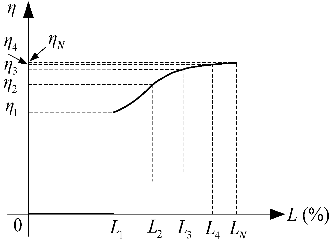
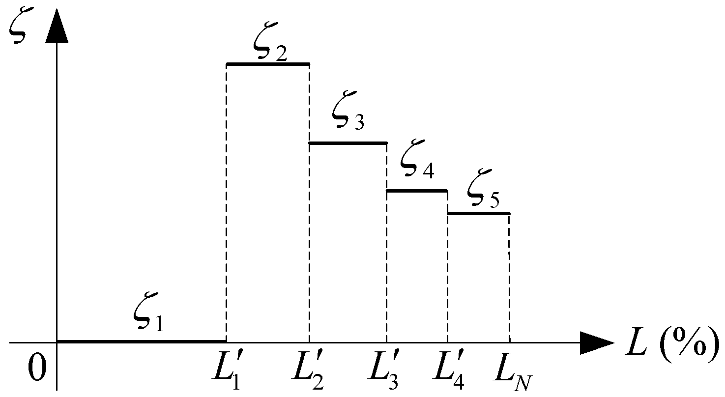
In actual application of CHPs, η is described with a series of data from field test. A discrete method is proposed to solve the optimization model. In this paper, the typical loading levels in Figure 2 and Figure 3 are shown in Table 1.

Table 1. Typical loading levels in Figure 2 and Figure 3.

Typical Loading Levels in Figure 2		Typical Loading Levels in Figure 3
$L_1$	40	$L_1^{\prime }$	40
$L_2$	65	$L_2^{\prime }$	60
$L_3$	78	$L_3^{\prime }$	80
$L_4$	90	$L_4^{\prime }$	90
$L_{\text{N}}$	100	$L_{\text{N}}$	100

Table 1. Typical loading levels in Figure 2 and Figure 3.

Typical Loading Levels in Figure 2		Typical Loading Levels in Figure 3
$L_1$	40	$L_1^{\prime }$	40
$L_2$	65	$L_2^{\prime }$	60
$L_3$	78	$L_3^{\prime }$	80
$L_4$	90	$L_4^{\prime }$	90
$L_{\text{N}}$	100	$L_{\text{N}}$	100

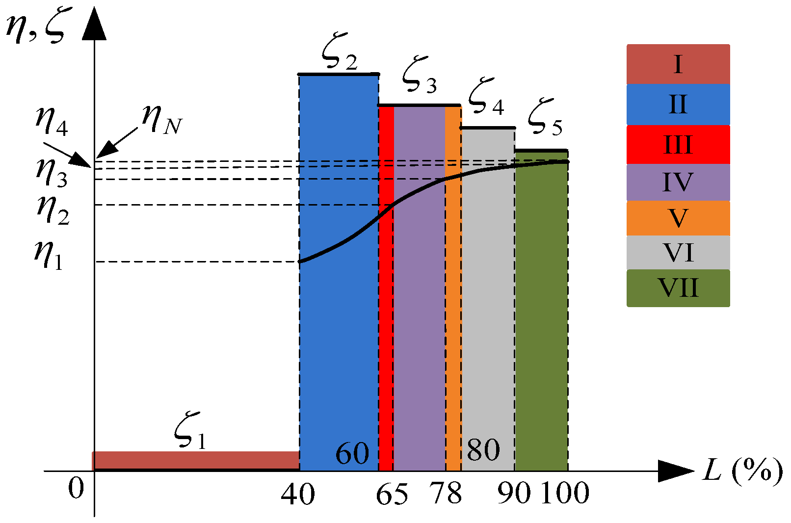
By combining Figure 2 and Figure 3, the relation between $\mathsf{\zeta }$ and η is rather clear, as shown in Figure 5. In Figure 5, there are mainly seven intervals where CHP could be operated at corresponding efficiency and HTPR. The seven intervals are shown in Table 2.

Figure 5. Optimization intervals division.

Figure 5. Optimization intervals division.

Table 2. Operation intervals for CHP. Heat to power ratios: HTPR.

Intervals	Overall Efficiency	HTPR	Interval type
I	f1(L)	ζ1	Zero
II	f2(L)	ζ2	Non-zero
III	f2(L)	ζ3	Non-zero
IV	f3(L)	ζ3	Non-zero
V	f4(L)	ζ3	Non-zero
VI	f4(L)	ζ4	Non-zero
VII	f5(L)	ζ5	Non-zero

Table 2. Operation intervals for CHP. Heat to power ratios: HTPR.

Intervals	Overall Efficiency	HTPR	Interval type
I	f1(L)	ζ1	Zero
II	f2(L)	ζ2	Non-zero
III	f2(L)	ζ3	Non-zero
IV	f3(L)	ζ3	Non-zero
V	f4(L)	ζ3	Non-zero
VI	f4(L)	ζ4	Non-zero
VII	f5(L)	ζ5	Non-zero

In Table 2, there are one zero interval (Interval I) and six non-zero intervals (from Interval II to Interval VII). In the $k\text{th}$ dispatching step, the forecasted $p_{\text{H}}\left(k\right)$, $p_{\text{E}}\left(k\right)$ and $p_{\text{G}}\left(k\right)$ are all constant. Through solving Equation (17) in the six non-zero intervals, respectively, the maximum profit for each interval will be obtained.

Take the case in Interval II as an example. In this interval, a fixed step of L is adopted, which is denoted by ${\mathrm{\Delta }}_{L_I}$. Then a series profit can be obtained, shown as:

$$\{\begin{array}{l}{\text{PRO}}_{\text{CHP\_base}}\left(k,40\%\right)=\frac{{\mathsf{\zeta }}_2}{1+{\mathsf{\zeta }}_2}q{\mathsf{\eta }}_1{p}_{\text{H}}\left(k\right)+\frac{1}{1+{\mathsf{\zeta }}_2}q{\mathsf{\eta }}_1{p}_{\text{E}}\left(k\right)-p_{\text{Gas}}\left(k\right)\hfill \\ {\text{PRO}}_{\text{CHP\_base}}\left(k,40\%+{\mathrm{\Delta }}_{L_I}\right)=\frac{{\mathsf{\zeta }}_2}{1+{\mathsf{\zeta }}_2}q{\text{f}}_2\left(40\%+{\mathrm{\Delta }}_{L_I}\right)p_H\left(k\right)+\frac{1}{1+{\mathsf{\zeta }}_2}q{\text{f}}_2\left(40\%+{\mathrm{\Delta }}_{L_I}\right)p_{\text{E}}\left(k\right)-p_{\text{Gas}}\left(k\right)\hfill \\ \begin{array}{cccc}\begin{array}{cccc}\begin{array}{cccc}& & & \end{array}& & & \end{array}& & \begin{array}{cccc}& & & \end{array}& ⋮\end{array}\hfill \\ {\text{PRO}}_{\text{CHP\_base}}\left(k,65\%\right)=\frac{{\mathsf{\zeta }}_2}{1+{\mathsf{\zeta }}_2}q{\text{f}}_2\left(65\%\right)p_{\text{H}}\left(k\right)+\frac{1}{1+{\mathsf{\zeta }}_2}q{\text{f}}_2\left(65\%\right)p_{\text{E}}\left(k\right)-p_{\text{Gas}}\left(k\right)\hfill \end{array}$$

(22)

The results obtained from Equation (22) failing to satisfy Equations (18)–(21) are deleted first, and then the maximum profit for Interval II is obtained and denoted by ${\text{PRO}}_{\text{CHP\_base,max}}^{\left(\text{II}\right)}\left(k\right)$.

The steps of L in each interval are usually different, which is determined by the loading level resolution of the field test results. The maximum profits for the other intervals are calculated similar to that of Interval II.

Then the maximum profit of the $k\text{th}$ dispatching step can be expressed as:

$${\text{PRO}}_{\text{CHP\_base,max}}\left(k\right)=\max \left\{{\text{PRO}}_{\text{CHP\_base,max}}^{\left(i\right)}\left(k\right),i=II,III,\cdots ,VII\right\}$$

(23)

where ${\text{PRO}}_{\text{CHP\_base,max}}\left(k\right)$ is the maximum value of ${\text{PRO}}_{\text{CHP\_base}}\left(k\right)$ in the $k\text{th}$ dispatching step; ${\text{PRO}}_{\text{CHP\_base,max}}^{\left(i\right)}\left(k\right)$ is the maximum value of ${\text{PRO}}_{\text{CHP\_base}}\left(k\right)$ in the $i\text{th}$ interval.

4.3. Dynamic Programming

Based on the forecasted prices of heat, electricity, and natural gas, the indication optimal operation points for CHP in one day can be obtained and corresponding operating schedules are pre-developed. Since the actual prices for each dispatching step are known at its beginning, certain modification has to be made to the operating schedule to obtain the actual maximum profits for CHP.

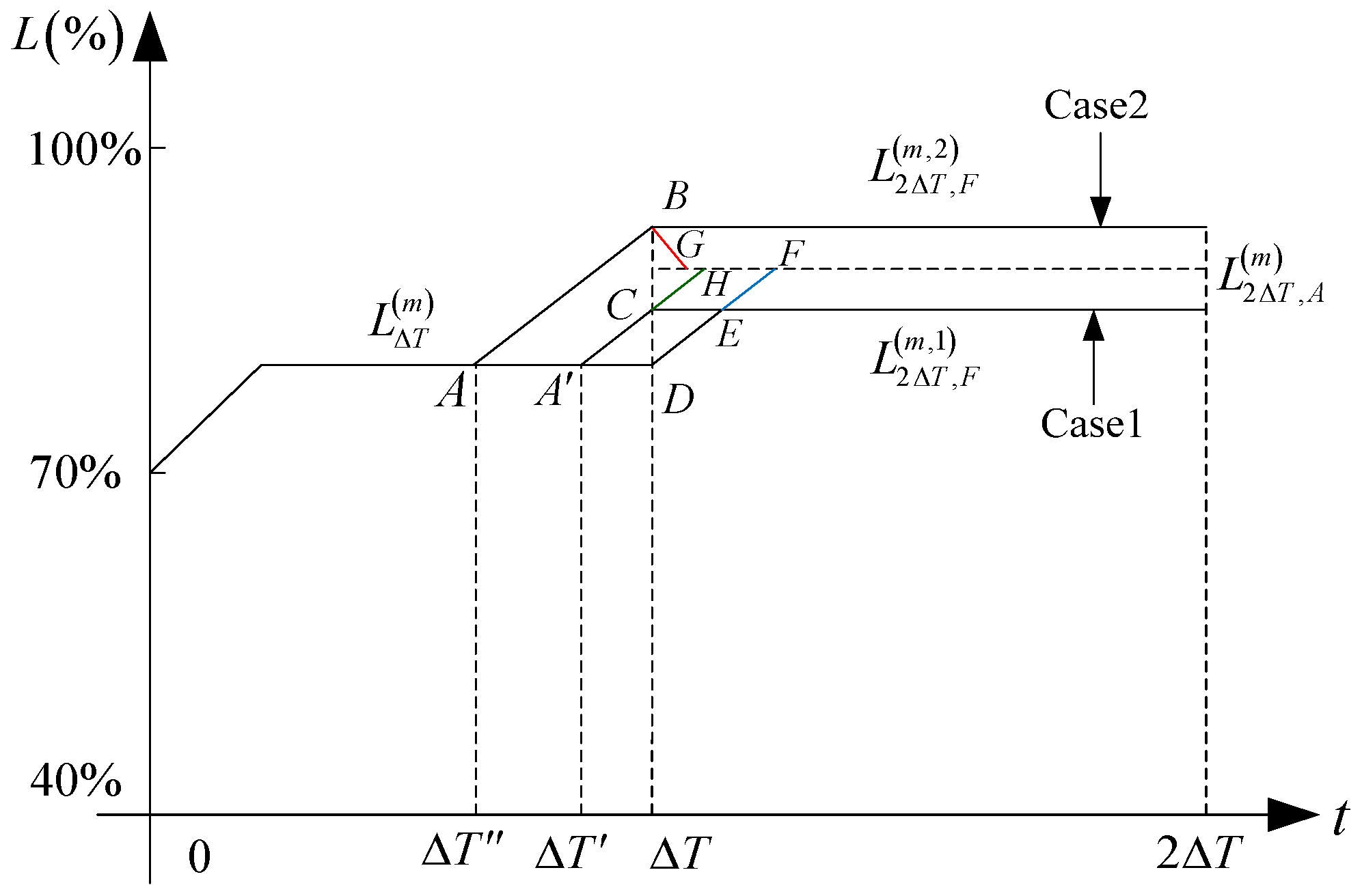
From ΔT to 2ΔT, the optimal operation points with maximum profits are obtained first based on forecasted prices. Around ΔT, the loading level is to be modified to the optimal loading level of the following dispatching step. The whole process is presented in Figure 6. $L_{\mathrm{\Delta }\text{T}}^{\left(m\right)}$ is the optimal loading level obtained based on the actual prices of 0–ΔT, where the profit of CHP is the maximum. The loading level is modified from 70% to $L_{\mathrm{\Delta }\text{T}}^{\left(m\right)}$ at the ramp rate of CHP. At ΔT, the actual prices for ΔT–2ΔT are known immediately and the corresponding optimal loading level is $L_{2\mathrm{\Delta }\text{T,A}}^{\left(m\right)}$. The load has the characteristic of retaining unchanged during a short period, which is reflected as the retaining characteristic of price. Thus, the CHP should be modified to the target optimal operation point when it is different from the current one.

Figure 6. Dynamic modification of CHP based on actual and forecasted prices.

Figure 6. Dynamic modification of CHP based on actual and forecasted prices.

For different relationship between the actual prices and forecasted prices, the actual maximum loading level may be higher or lower than the forecasted maximum loading level, named as Case 1 and Case 2, respectively.

4.3.1. Case 1

In Case 1, the forecasted optimal loading level $L_{2\mathrm{\Delta }\text{T,F}}^{\left(m,1\right)}$, obtained from the revised forecasted prices, is lower than $L_{2\mathrm{\Delta }\text{T,A}}^{\left(m\right)}$. There are two potential operation routes:

■

In the first route, $L_{\mathrm{\Delta }\text{T}}^{\left(m\right)}$ is modified to $L_{2\mathrm{\Delta }\text{T,F}}^{\left(m,1\right)}$ in advance, and then modified to $L_{2\mathrm{\Delta }\text{T,A}}^{\left(m\right)}$ at ΔT directly.

■

In the second route, CHP is operated at $L_{\mathrm{\Delta }\text{T}}^{\left(m\right)}$ until ΔT, and then modified to $L_{2\mathrm{\Delta }\text{T,A}}^{\left(m\right)}$ directly.

To decide which route is better, the profit during the two modification processes should be calculated first. The two routes are denoted by $A^{\prime }\to C\to H\to F$ and $A^{\prime }\to D\to E\to F$, respectively.

(1) Route $A^{\prime }\to C\to H\to F$

In 0–ΔT, the pre-modification time ΔT’ can be calculated as follows:

$$\mathrm{\Delta }{T}^{\prime }=\left(L_{2\mathrm{\Delta }\text{T,F}}^{\left(m,1\right)}-L_{\mathrm{\Delta }\text{T}}^{\left(m\right)}\right)/{\mathsf{\delta }}_{\text{L}}$$

(24)

where ${\mathsf{\delta }}_{\text{L}}$ is the ramp rate and ${\mathsf{\delta }}_{\text{L}}={\mathsf{\tau }}_{\text{ramp}}/S_{\text{N}}$.

At ΔT, the loading level is modified to $L_{2\mathrm{\Delta }\text{T,A}}^{\left(m\right)}$ directly and ends at F. The overall profit during the modification process from A’ to F is:

$$\text{PR}{\text{O}}_{\text{A}}^{\left(1\right)}={\displaystyle \sum _{A^{\prime }\to C}{\text{PRO}}^{\left(\mathrm{\Delta }\text{T}\right)}\left(L\right)+}{\displaystyle \sum _{C\to H\to F}{\text{PRO}}^{\left(2\mathrm{\Delta }\text{T}\right)}\left(L\right)}$$

(25)

where ${\text{PRO}}^{\left(\mathrm{\Delta }\text{T}\right)}\left(L\right)$ is the profit-loading curve in 0–ΔT, ${\text{PRO}}^{\left(2\mathrm{\Delta }\text{T}\right)}\left(L\right)$ is the profit-loading curve in ΔT–2ΔT.

(2) Route $A^{\prime }\to D\to E\to F$

The loading level keeps unmodified until D and modified to $L_{2\mathrm{\Delta }\text{T},\text{A}}^{\left(m\right)}$. During the whole process, the forecast optimal loading level $L_{2\mathrm{\Delta }\text{T,F}}^{\left(m,1\right)}$ does not affect the operating schedule. The overall profit is:

$${\text{PRO}}_{\text{B}}^{\left(1\right)}={\displaystyle \sum _{A^{\prime }\to D}{\text{PRO}}^{\left(\mathrm{\Delta }\text{T}\right)}\left(L\right)+}{\displaystyle \sum _{D\to E\to F}{\text{PRO}}^{\left(2\mathrm{\Delta }\text{T}\right)}\left(L\right)}$$

(26)

Based on ${\text{PRO}}_{\text{A}}^{\left(1\right)}$ and ${\text{PRO}}_{\text{B}}^{\left(1\right)}$, the optimal modification route with the maximum profit can then be determined.

If ${\text{PRO}}_{\text{A}}^{\left(1\right)}>{\text{PRO}}_{\text{B}}^{\left(1\right)}$, the CHP is modified according to $A^{\prime }\to C\to H\to F$.

If ${\text{PRO}}_{\text{A}}^{\left(1\right)}<{\text{PRO}}_{\text{B}}^{\left(1\right)}$, the CHP is modified according to $A^{\prime }\to D\to E\to F$.

4.3.2. Case 2

In Case 2, the forecast optimal loading level is $L_{2\mathrm{\Delta }\text{T,F}}^{\left(m,2\right)}$, which is also obtained from the revised forecasted prices, is higher than $L_{2\mathrm{\Delta }\text{T,A}}^{\left(m\right)}$. There are also two potential operation routes.

■

In the first route, $L_{\mathrm{\Delta }\text{T}}^{\left(m\right)}$ is pre-modified to $L_{2\mathrm{\Delta }\text{T,F}}^{\left(m,2\right)}$, and then decreased to $L_{2\mathrm{\Delta }\text{T,A}}^{\left(m\right)}$ at ΔT.

■

In the second route, CHP is operated at $L_{\mathrm{\Delta }\text{T}}^{\left(m\right)}$ until ΔT, and then modified to $L_{2\mathrm{\Delta }\text{T,A}}^{\left(m\right)}$. The second route is almost the same with that in Case 1.

The two routes are denoted by $A\to B\to G\to F$ and $A\to D\to E\to F$, respectively.

(1) Route $A\to B\to G\to F$

In 0–ΔT, the pre-modification time ΔT’’ is determined as follows:

$$\mathrm{\Delta }{T}^{″}=\left(L_{2\mathrm{\Delta }\text{T,F}}^{\left(m,2\right)}-L_{\mathrm{\Delta }\text{T}}^{\left(m\right)}\right)/{\mathsf{\delta }}_{\text{L}}$$

(27)

The actual prices for ΔT–2ΔT are known at B. Then the loading level of CHP is modified to G and ended at F. The overall profit for the modification process is expressed as:

$${\text{PRO}}_{\text{A}}^{\left(2\right)}={\displaystyle \sum _{A\to B}{\text{PRO}}^{\left(\mathrm{\Delta }\text{T}\right)}\left(L\right)+}{\displaystyle \sum _{B\to G\to F}{\text{PRO}}^{\left(2\mathrm{\Delta }\text{T}\right)}\left(L\right)}$$

(28)

(2) Route $A\to D\to E\to F$

The route is almost same with that in Case 1, with a different beginning point A. The overall profit for the modification process is calculated by:

$${\text{PRO}}_{\text{B}}^{\left(2\right)}={\displaystyle \sum _{A\to D}{\text{PRO}}^{\left(\mathrm{\Delta }\text{T}\right)}\left(L\right)+}{\displaystyle \sum _{D\to E\to F}{\text{PRO}}^{\left(2\mathrm{\Delta }\text{T}\right)}\left(L\right)}$$

(29)

Based on ${\text{PRO}}_{\text{A}}^{\left(2\right)}$ and ${\text{PRO}}_{\text{B}}^{\left(2\right)}$, the optimal modification route can be obtained.

If ${\text{PRO}}_{\text{A}}^{\left(2\right)}>{\text{PRO}}_{\text{B}}^{\left(2\right)}$, the CHP is modified according to $A\to B\to G\to F$.

If ${\text{PRO}}_{\text{A}}^{\left(2\right)}<{\text{PRO}}_{\text{B}}^{\left(2\right)}$, the CHP is modified according to $A\to D\to E\to F$.

The same way is applied to each 2ΔT time window, which starts at $k\mathrm{\Delta }T$ and ends at $\left(k+2\right)\mathrm{\Delta }T$, to obtain the optimal modification route for one day. During the whole process, the price forecasting is considered, which is more practical in real-time markets.

5. Demonstration Examples

In this paper, a 1 MW CHP is optimized based on the proposed method. The other technical parameters of the CHP are presented in

Table A1. Technical parameters of CHP.

Nominal capacity SN (MW)			1
Ramp Capacity τramp (kW/min)			15
Electricity Output (MW)			0.7 (max)		0.4 (mini)
Heat Output (MW)			0.6 (max)		0.3 (mini)
Typical Overall Efficiency		Loading Level	HTPR		Loading Level
η1	80%	40%	ζ1	0		0%–40%
η2	85%	65%	ζ2	2.83		40%–60%
η3	86.7%	78%	ζ3	2.2		60%–80%
η4	87.5%	90%	ζ4	1.4		80%–90%
ηN	87.8%	100%	ζ5	0.8		90%–100%

.

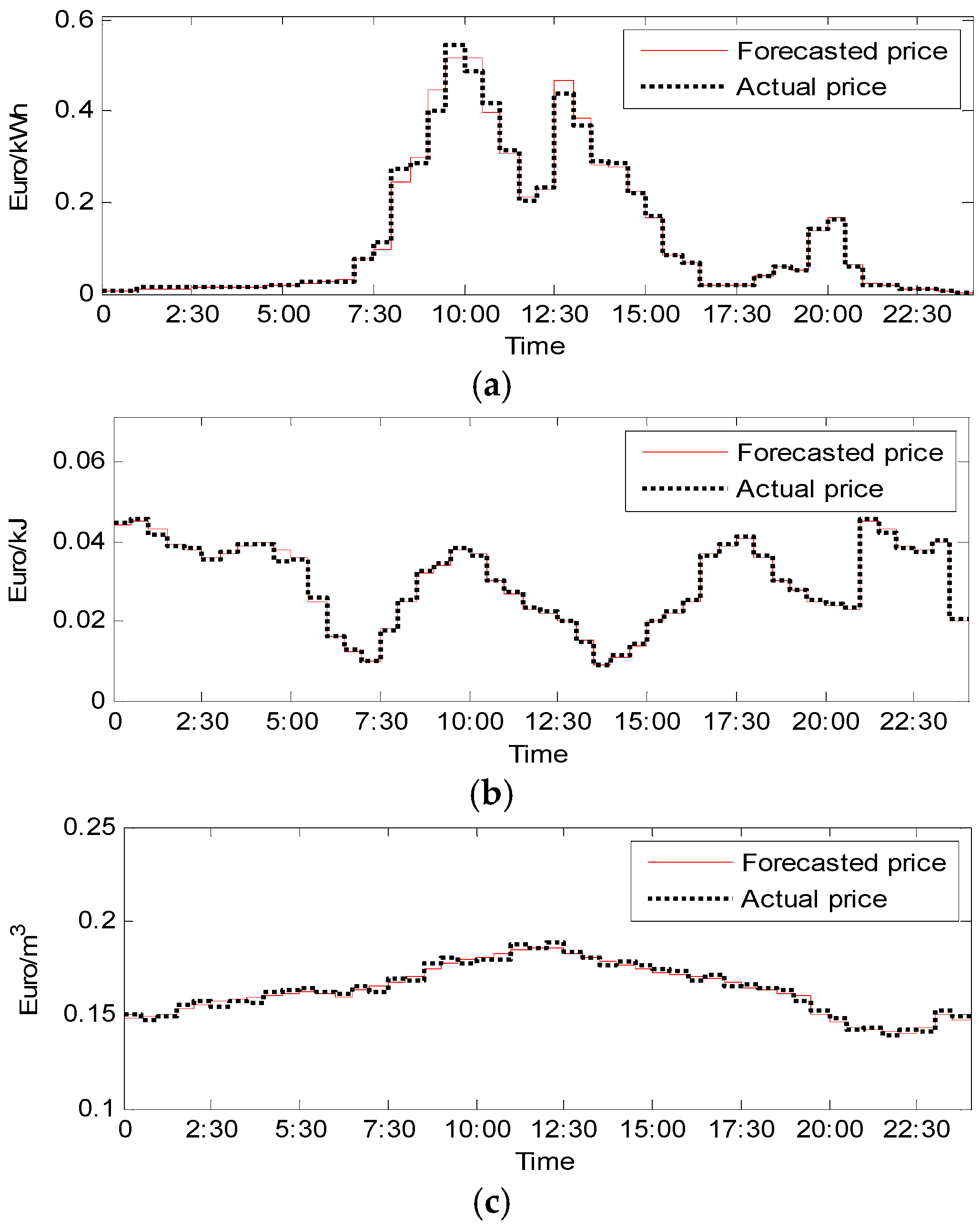
The prices of electricity, heat, and natural gas are forecasted by using the gray forecasting model and revised in real-time with the least square method, where the actual prices are from [28]. The results are shown in Figure 7.

As shown in Figure 7, the energy prices are forecasted accurately by using the proposed method. The variances between the actual and forecasted price of electricity, heat and gas are 0.023, 0.00011, and 0.00018, respectively. In Figure 7a, the forecasted price is almost the same with its actual value when the price curve is flat, between 0:00 and 7:00, 16:00 and 19:30, 21:00 and 24:00 When the price changes suddenly, which reflects the sudden change of the electric loads, there will exist certain error between the actual and forecasted prices. The case happens at 10:00 and 13:00. The similar phenomenon also occurs in Figure 7b,c.

Figure 7. Actual and forecasted prices of electricity, heat, and natural gas. (a) Electricity price; (b) heat price; and (c) natural gas price.

Figure 7. Actual and forecasted prices of electricity, heat, and natural gas. (a) Electricity price; (b) heat price; and (c) natural gas price.

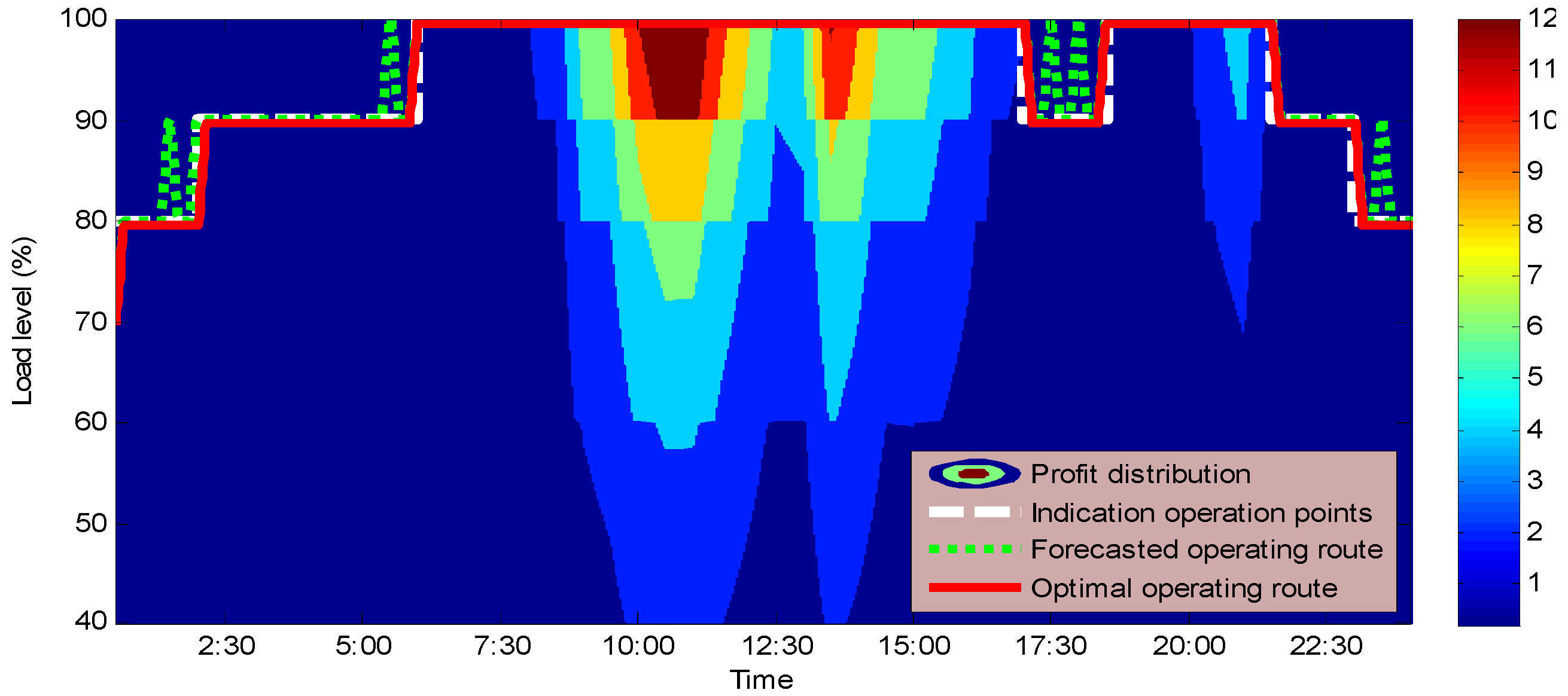
Based on the actual and forecasted prices, the optimal operation points, where the profits of CHP reach their maximum, are obtained and shown in Figure 8. At 0:00, The CHP is operated at the loading level of 70%, which is obtained from the day-ahead operating data. In Figure 8, the profits of CHP operated at different loading levels at different time in one day are presented. The white dotted line is the indication operation points for CHP in one day, which is obtained based on actual prices.

From Figure 8, it can be found that the maximum profit occurs at 10:00, about 12 Euro shown in deep red, when the CHP is in full load. The relatively high profit for CHP is between 8:00 and 16:00, 20:00 and 21:00. From Figure 7, it is found the electric price is much higher than that of heat in between 8:00 and 16:00 and, thus, the profit of CHP is relatively higher than other time. Between 0:00 and 8:00, 16:00 and 20:00, when the electric price is the same with or lower than heat price, the profits for CHP are relatively low. So the profit of CHP is mainly determined by the electric price, for its usually high value than heat.

Figure 8. Profit distribution of the CHP.

Figure 8. Profit distribution of the CHP.

Based on the indication operation points, specific operation schedule can be developed after considering the ramp constraints. The green dotted line in Figure 8 is the forecasted operating route obtained from the forecasted prices. The red line in Figure 8 in is the optimal operating route obtained from the proposed dynamic programming method. It can be found that the red line and the white dotted line almost coincide with each other. Namely, the optimized profits comply quite well with those derived from actual conditions. At 1:30, the loading level for maximum profit point got from the forecasted prices is 90%, and it is modified to 90% before 1:30. However, the loading level for the maximum profit point got from the actual price is 80% at 1:30, thus the loading level has to be modified back to 80%. During the process, a lot of profits are lost for CHP. The optimal operating route is staying unchanged, as shown in the red line. At 2:30, the operating route is modifying CHP before 2:30 in the green dotted line, while the optimal route is modifying CHP after 2:30, shown in the red line. Sometimes, the operating route obtained from the forecasted prices happen to be the optimal one, such as at 6:30, 16:30, 19:00, 21:30, and 22:30. Take the case at 6:00 as an example, the loading level of CHP should be modified to 100% before 6:30, and the results of the green dotted line are consistent with that of the red line. The profits of the routes in green and red are shown in Table 3, respectively.

From Table 3, it can be found that the profits for CHP of the optimal route reach their maximum. The maximum profit in one day is about 14 Euro, between 10:00 and 11:00. The maximum profit is just about 1 Euro in the deep night. The high loading level for CHP does not mean high profits, either. Between 0:00 and 2:30, 2:30 and 6:00, the CHP is operated at the loading level of 80% and 90% to obtain the maximum profits. The similar case occurs between 16:00 and 18:00, 21:00 and 24:00. The reason is that the price of electricity is low and the CHP is operated at relatively low loading level to gain a high value of HTPR.

Table 3. Maximum profits of the forecasted route and optimal route.

Time	Maximum Profit from the Forecasted Route (Euro)	Maximum Profit from the Optimal Route (Euro)	Time	Maximum Profit from the Forecasted Route (Euro)	Maximum Profit from the Optimal Route (Euro)
0:30	1.01	1.01	12:30	6.11	6.11
1:00	1.05	1.07	13:00	12.37	12.37
1:30	1.00	1.03	13:30	10.13	10.13
2:00	0.97	0.97	14:00	7.30	7.30
2:30	0.95	0.95	14:30	7.24	7.24
3:00	0.95	0.95	15:00	5.93	5.93
3:30	0.95	0.95	15:30	4.52	4.52
4:00	1.01	1.01	16:00	2.38	2.38
4:30	1.04	1.04	16:30	2.05	2.05
5:00	1.01	1.03	17:00	0.98	0.99
5:30	0.97	1.00	17:30	1.05	1.08
6:00	0.92	0.95	18:00	1.12	1.15
6:30	0.81	0.81	18:30	1.54	1.54
7:00	0.81	0.81	19:00	1.91	1.91
7:30	1.98	1.98	19:30	1.74	1.74
8:00	2.67	2.67	20:00	3.88	3.88
8:30	6.71	6.71	20:30	4.64	4.64
9:00	8.15	8.15	21:00	1.94	1.94
9:30	12.09	12.09	21:30	1.27	1.27
10:00	14.05	14.05	22:00	1.18	1.18
10:30	14.03	14.03	22:30	0.99	0.99
11:00	10.70	10.70	23:00	0.88	0.90
11:30	8.29	8.29	23:30	0.91	0.93
12:00	5.74	5.74	24:00	0.38	0.38

Table 3. Maximum profits of the forecasted route and optimal route.

Time	Maximum Profit from the Forecasted Route (Euro)	Maximum Profit from the Optimal Route (Euro)	Time	Maximum Profit from the Forecasted Route (Euro)	Maximum Profit from the Optimal Route (Euro)
0:30	1.01	1.01	12:30	6.11	6.11
1:00	1.05	1.07	13:00	12.37	12.37
1:30	1.00	1.03	13:30	10.13	10.13
2:00	0.97	0.97	14:00	7.30	7.30
2:30	0.95	0.95	14:30	7.24	7.24
3:00	0.95	0.95	15:00	5.93	5.93
3:30	0.95	0.95	15:30	4.52	4.52
4:00	1.01	1.01	16:00	2.38	2.38
4:30	1.04	1.04	16:30	2.05	2.05
5:00	1.01	1.03	17:00	0.98	0.99
5:30	0.97	1.00	17:30	1.05	1.08
6:00	0.92	0.95	18:00	1.12	1.15
6:30	0.81	0.81	18:30	1.54	1.54
7:00	0.81	0.81	19:00	1.91	1.91
7:30	1.98	1.98	19:30	1.74	1.74
8:00	2.67	2.67	20:00	3.88	3.88
8:30	6.71	6.71	20:30	4.64	4.64
9:00	8.15	8.15	21:00	1.94	1.94
9:30	12.09	12.09	21:30	1.27	1.27
10:00	14.05	14.05	22:00	1.18	1.18
10:30	14.03	14.03	22:30	0.99	0.99
11:00	10.70	10.70	23:00	0.88	0.90
11:30	8.29	8.29	23:30	0.91	0.93
12:00	5.74	5.74	24:00	0.38	0.38

6. Conclusions

In this paper, a SIMO model is established for CHP, whose overall efficiency and HTPR are both in variation with the loading level. To optimize the operation of CHP in the real-time market, the real-time prices of heat, electricity, and natural gas are forecasted. A dynamic programming method is also proposed to design the optimal operation. The conclusions are drawn and summarized as follows:

■

With the proposed method, the energy prices are forecasted, where the variances between actual and forecasted prices of electricity, heat and gas are only 0.023, 0.00011, and 0.00018, respectively. In addition, the optimized profits of the CHP obtained from modifying the pre-developed strategy comply well with actual conditions by using the proposed dynamic programming algorithm, as the red and white dotted lines shown in Figure 8.

■

In day time, the optimal operation routine is mainly dominated by high electric prices and high electric demand. The CHP should be operated at a high loading level to gain a relatively low HTPR (e.g., 0.8) to generate more electricity. At night, the optimal operation routine is mainly dominated by high heat price and high heat demand. The CHP should be operated at a low loading level to gain a high HTPR (e.g., 2.2) to generate more heat. Thus, it is found that high loading level or high output of CHP does not always produce high profits.