
Dual Search Maximum Power Point (DSMPP) Algorithm Based on Mathematical Analysis under Shaded Conditions

 , and
, and
Abstract
:1.Introduction
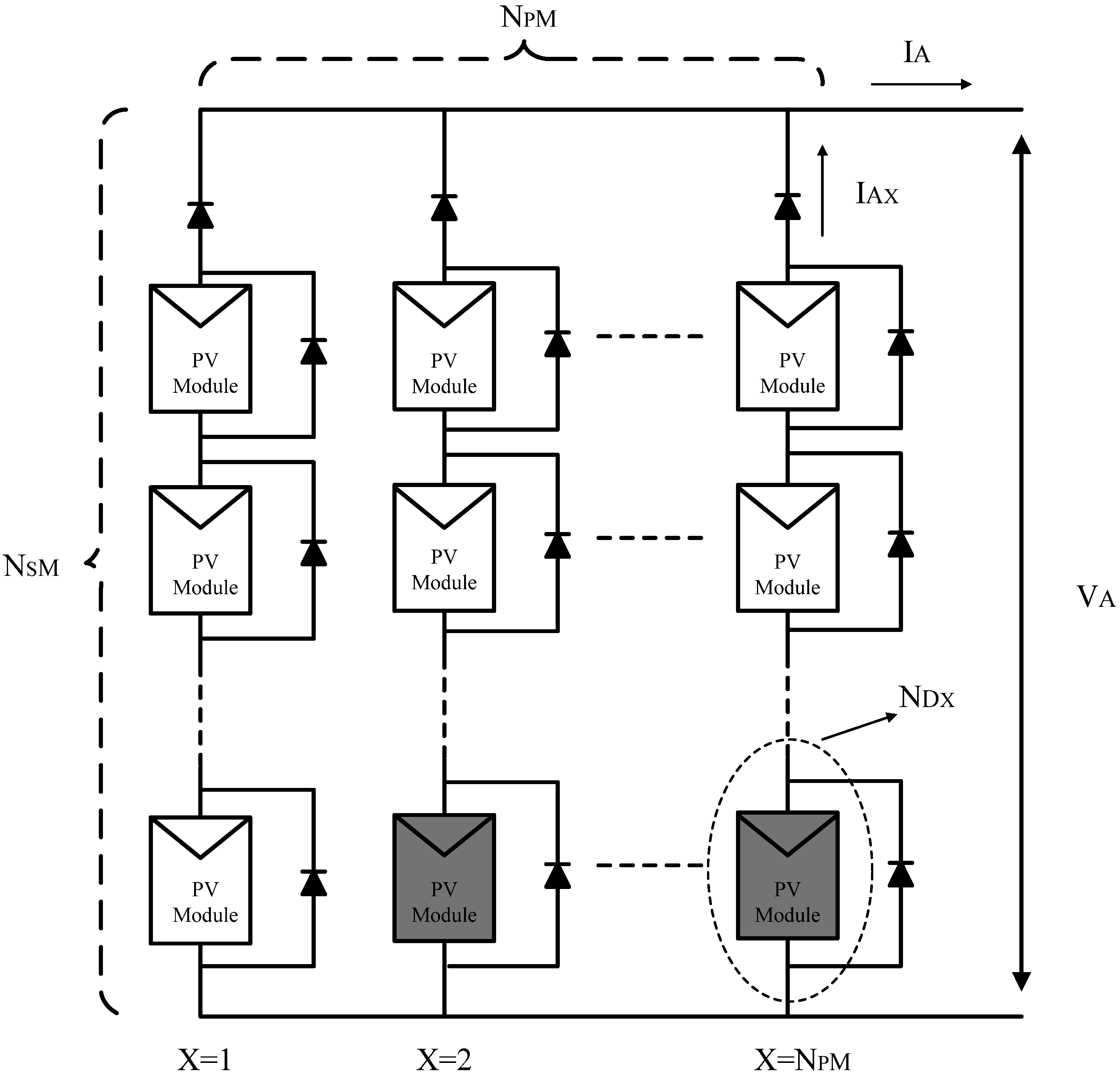
2. Photovoltaic (PV) System Model
2.1. PV Array Model under Uniform Conditions

2.2. Mathematical Model of PV Array under Uniform and Partially Shaded Conditions

3. DC-DC Boost Converter

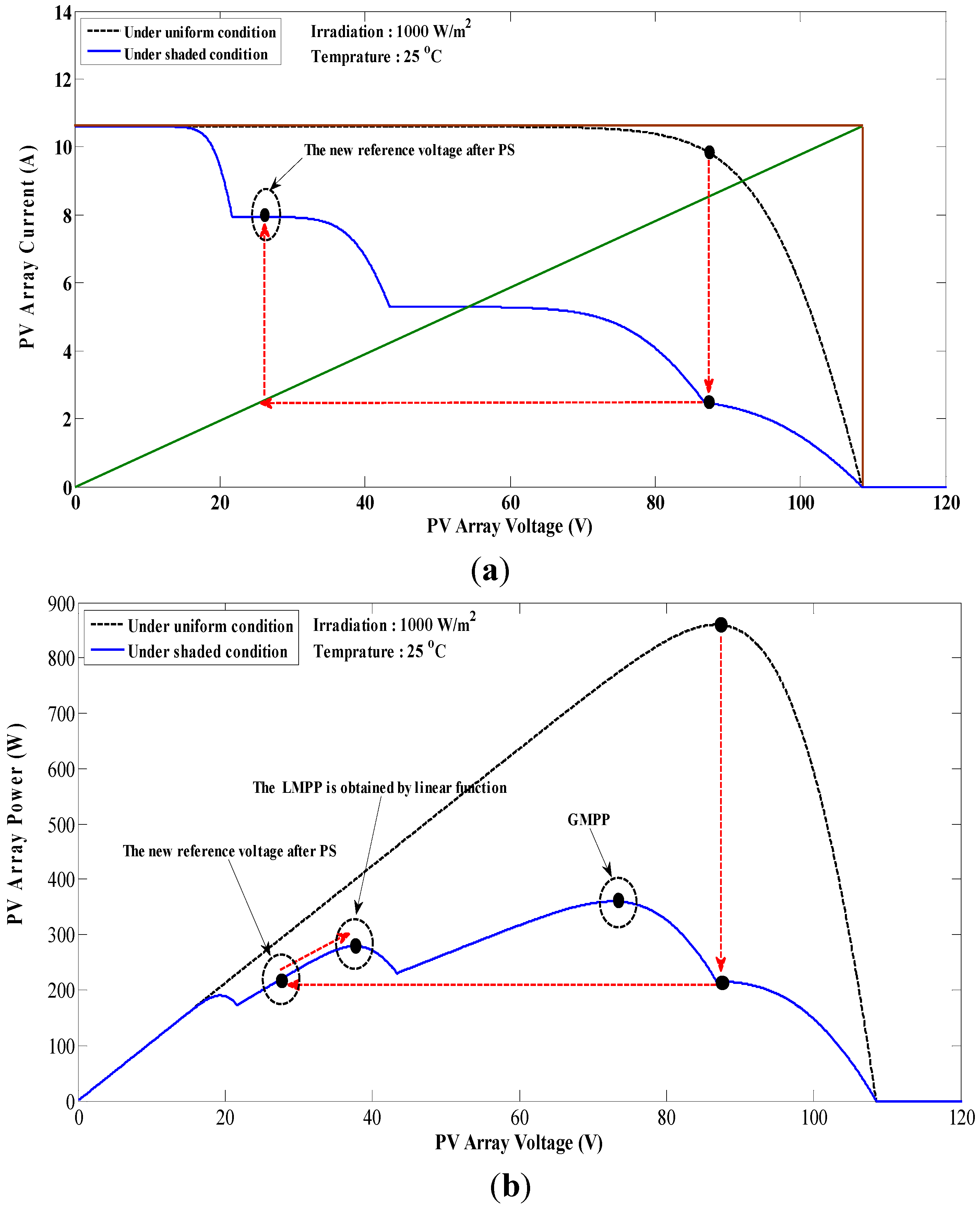
4. Maximum Power Point Tracking (MPPT) Based on a Linear
Function under Partially Shaded Conditions (PSC)


- (1)
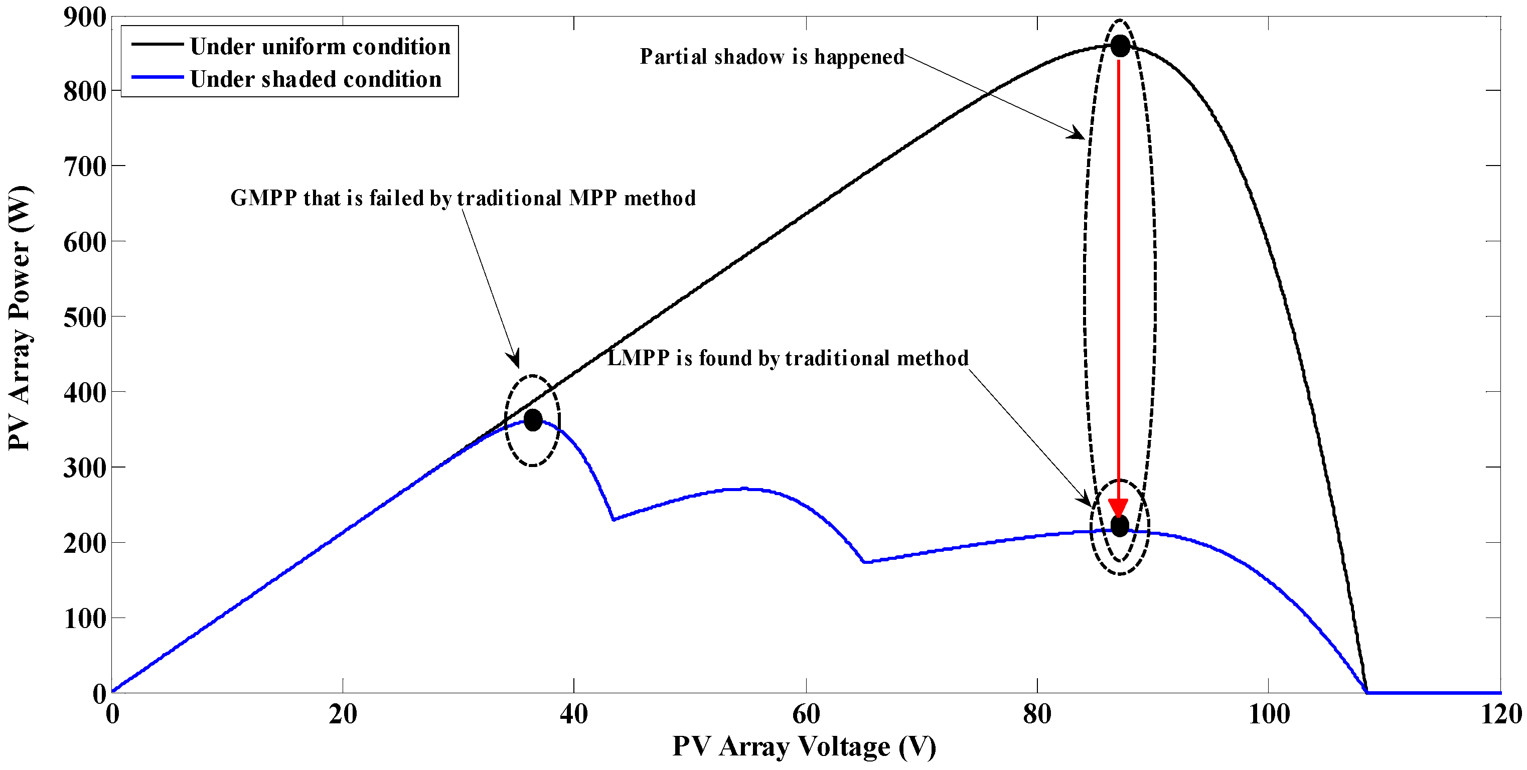
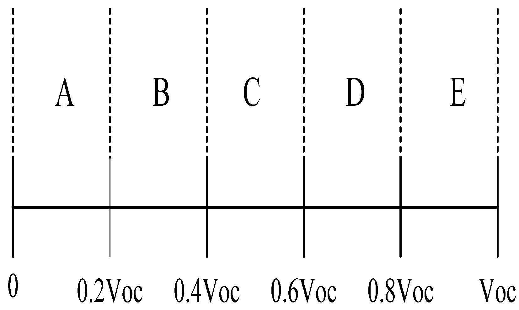
- The open-circuit voltage and short-circuit current methods are alternative techniques for obtaining the MPP. The open-circuit method is based on the relationship between the voltage of the PV array at the maximum power point (VMPP) and the open-circuit voltage of the PV array (VOCA). The short-circuit current method is based on the relationship between the current of the PV array at the MPP (IMPP) and the short-circuit current of the PV array (ISCA). In these methods, the voltage and current at the MPP are approximately 80% of the open-circuit voltage and 92% of the short-circuit current, respectively [44,45,46].
- (2)
- In PSCs with multi-peak power points, the distance between peak powers are integral multiples of 80% of the open-circuit of the PV module (n × 0.8 × VOC_Module), where n is an integer. If the minimum number of different levels of the shaded modules in the strings is one, then the minimum value of n is one. In other words, the minimum distance between two consecutive peaks is 0.8 × VOC_Module.

| Stage | 1 | 2 | 3 | 4 | 5 | |
|---|---|---|---|---|---|---|
| Parameter | ||||||
| nPS | 1 | 2 | 2 | 3 | 3 | |
| Vreff | 0.69VOCA | 0.46VOCA | 0.46VOCA | 0.23VOCA | 0.23VOCA | |
| nMPP | 2 | 2 | 3 | 2 | 4 | |
| K | 1, 2, 3, 4 | 3, 4 | 3, 4 | 4 | 4 | |
| IMPP_1 | 0.69ISCA | 0.46ISCA | 0.46ISCA | 0.23ISCA | 0.23ISCA | |
| VMPP_1 | 0.8VOCA | 0.8VOCA | 0.8VOCA | 0.8VOCA | 0.8VOCA | |
| PMPP_1 | 0.552VOCA×ISCA | 0.368VOCA×ISCA | 0.368VOCA×ISCA | 0.184VOCA×ISCA | 0.184VOCA×ISCA | |
| IMPP_2 | 0.92ISCA | 0.92ISCA | 0.69ISCA | 0.92ISCA | √ | |
| VMPP_2 | 0.48VOCA | 0.32VOCA | 0.32VOCA | 0.16VOCA | √ | |
| PMPP_2 | 0.44VOCA×ISCA | 0.294VOCA×ISCA | 0.22VOCA×ISCA | 0.147VOCA×ISCA | √ | |
| IMPP_3 | - | - | 0.92ISCA | - | √ | |
| VMPP_3 | - | - | 0.16VOCA | - | √ | |
| PMPP_3 | - | - | 0.147VOCA×ISCA | - | √ | |
| IMPP_4 | - | - | - | - | 0.92ISCA | |
| VMPP_4 | - | - | - | - | 0.16VOCA | |
| PMPP_4 | - | - | - | - | 0.147VOCA×ISCA | |

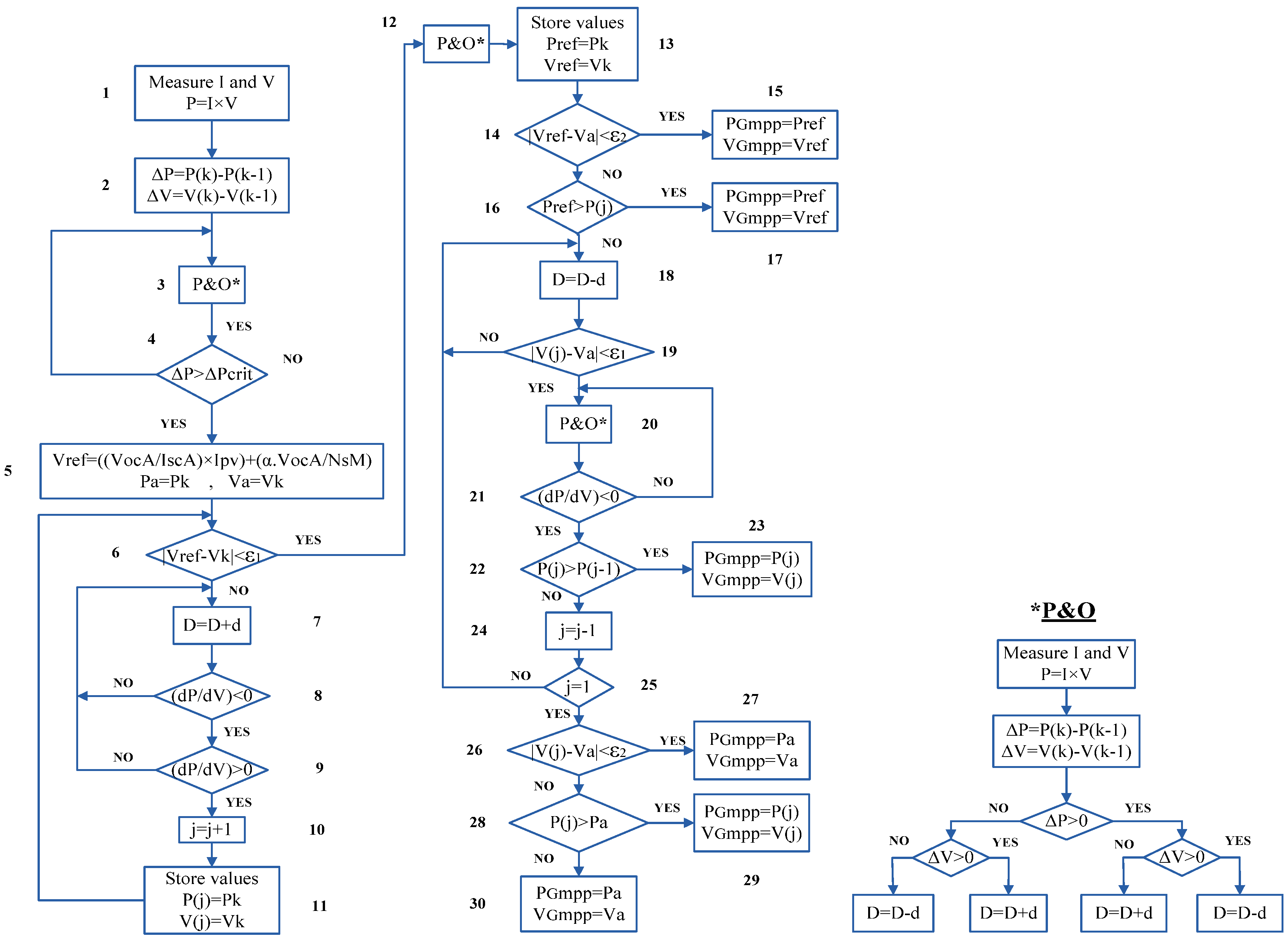
5. Proposed Dual Search MPPT Algorithm

- Based on the above-described analyses, the GMPP is not on the left side of the new reference voltage created by the modified linear function.
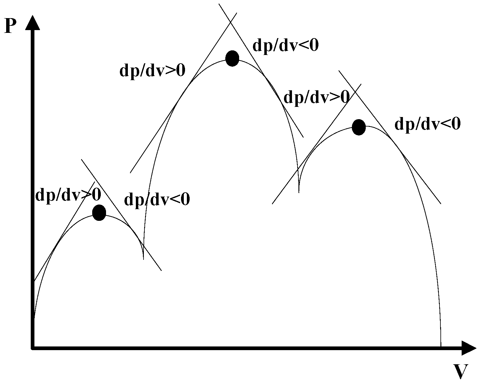
- In P-V curves with multi-peak powers, when the GMPP is obtained, the magnitude of the subsequent MPPs decreases from either side.
- The minimum distance between two consecutive MPPs is 0.8 × VOCM.
- When the duty cycle is the output of the P & O method, the PID controller is not needed, and consequently, the controller will be simplified.
- By carefully adjusting the step size of the duty cycle, the time required to reach the MPP and the overshoot and oscillations are significantly reduced, which can increase the efficiency of the system.
- In the modified linear function, the open-circuit voltage and the short-circuit current of the PV array are the most important parameters that should be updated by changing the irradiation to obtain the correct value of the new reference voltage.


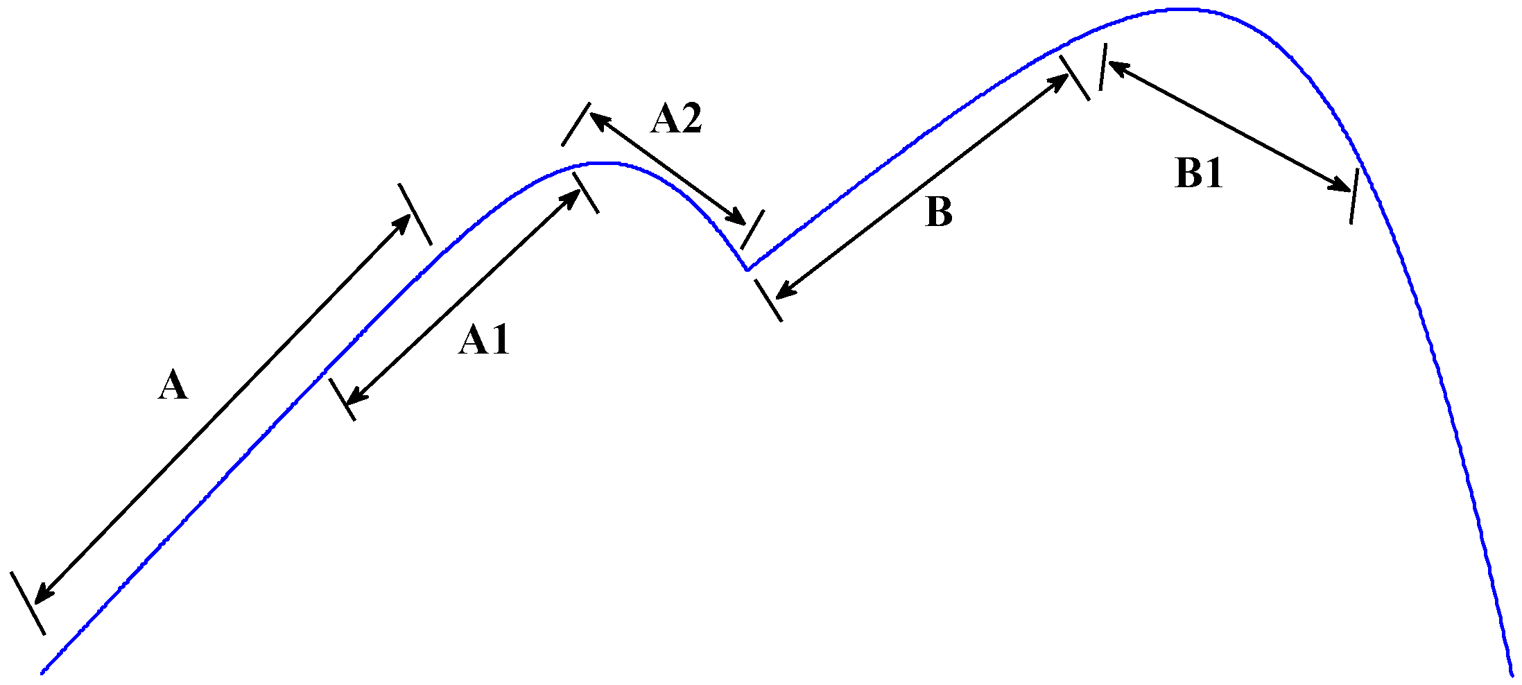
- (A)
- When PSCs do not occur, according to Equation (13), the PV voltage should increase rapidly to reach the MPP, and thus, a greater value of d is selected, which leads to a decrease in the time required to reach the MPP.
- (B)
- When the MPP under uniform condition or the GMPP under PSCs is obtained, the value of d should be adjusted to be lower so that the overshoot and oscillations can significantly be reduced.
- (C)
- Under PSCs, a large value of d should be selected to reach the operating point near the new reference voltage point, as calculated by Equation (19).
- (D)
- When the existing operating point is near the new reference voltage, such as in blocks 6 and 19, a small value of d should be selected to avoid missing the new operating point.
6. Simulation Results
| Parameters | Values |
|---|---|
| Power in maximum point, MPP | 43 W |
| Voltage in maximum point, VMPP | 17.4 V |
| Current in maximum point, IMPP | 2.48 A |
| Open circuit voltage, VOC | 21.7 V |
| Short circuit current, ISC | 2.65 A |
| Temperature coefficient of VOC | −0.0821 V/°C |
| Temperature coefficient of ISC | 0.00106 A/°C |
| Number of cells per module | 36 |


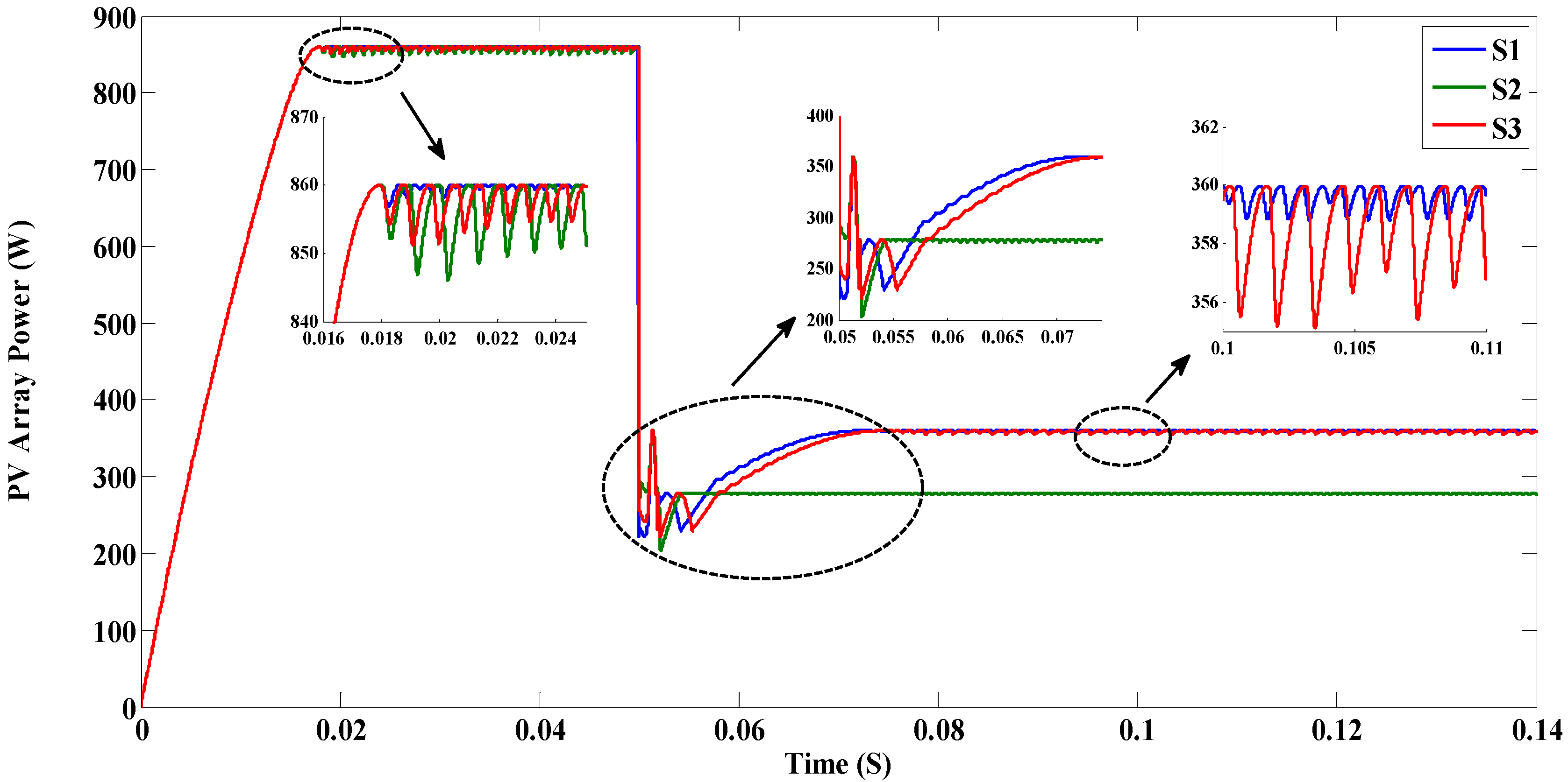
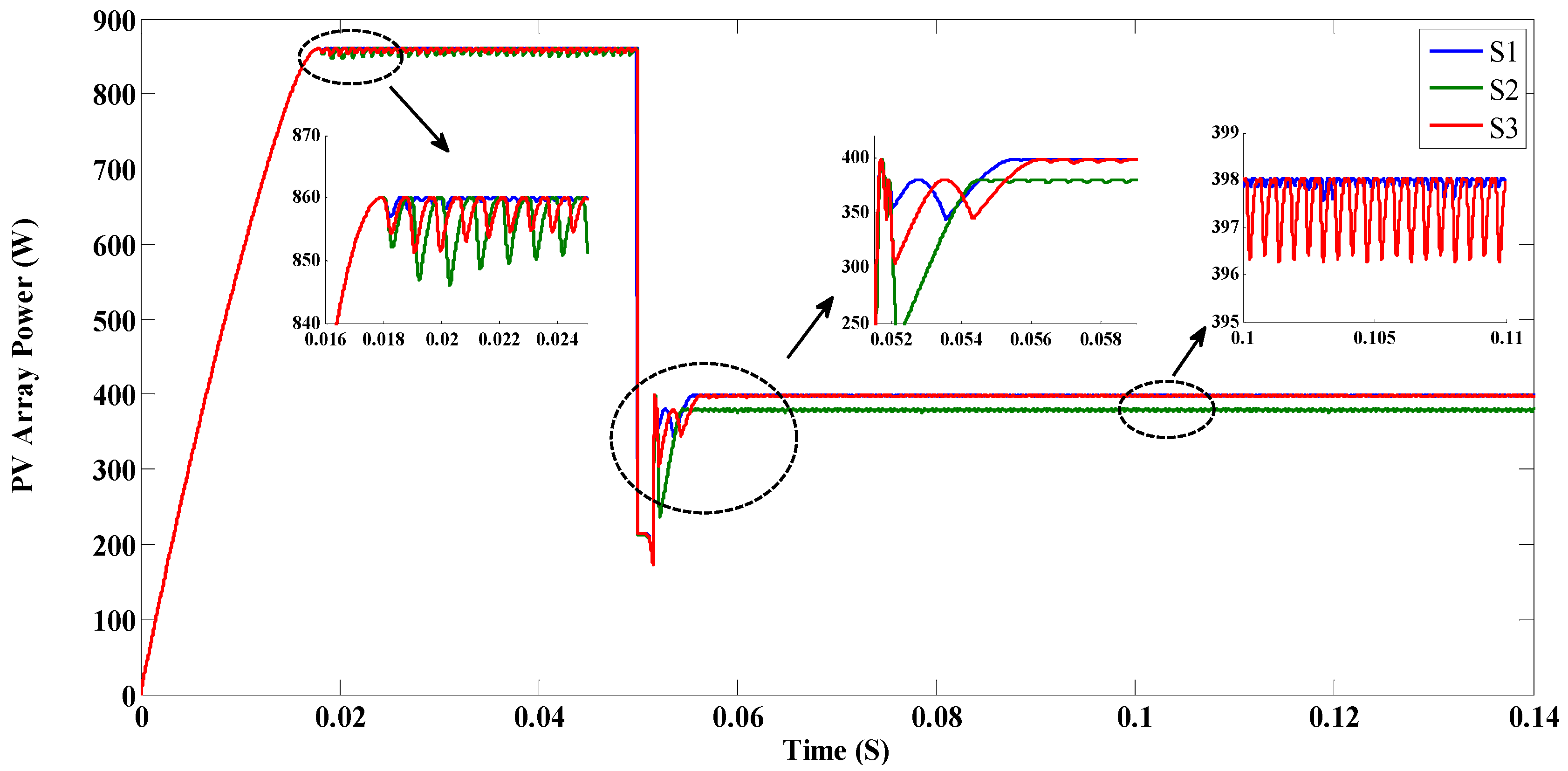
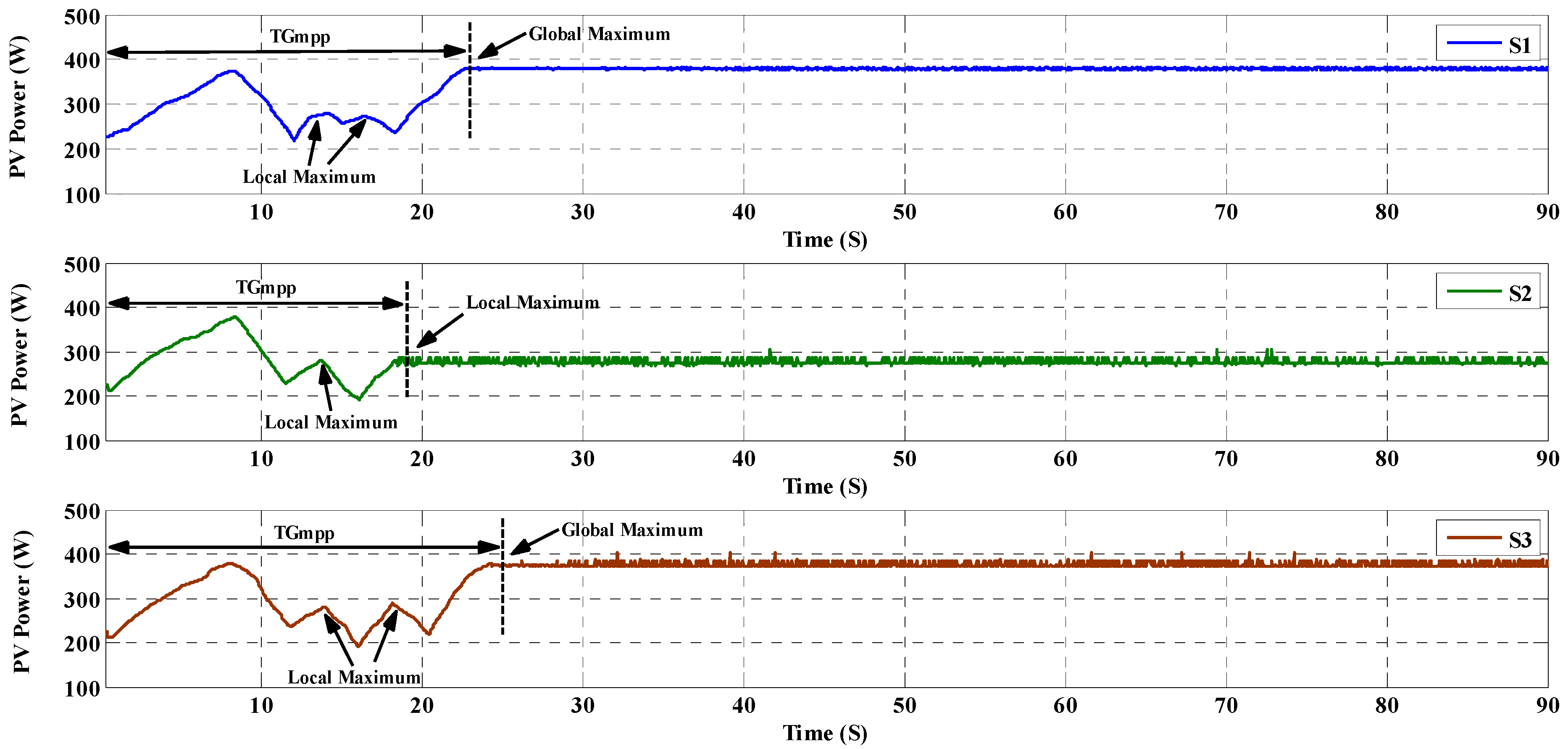
- SOP: Status of operation;
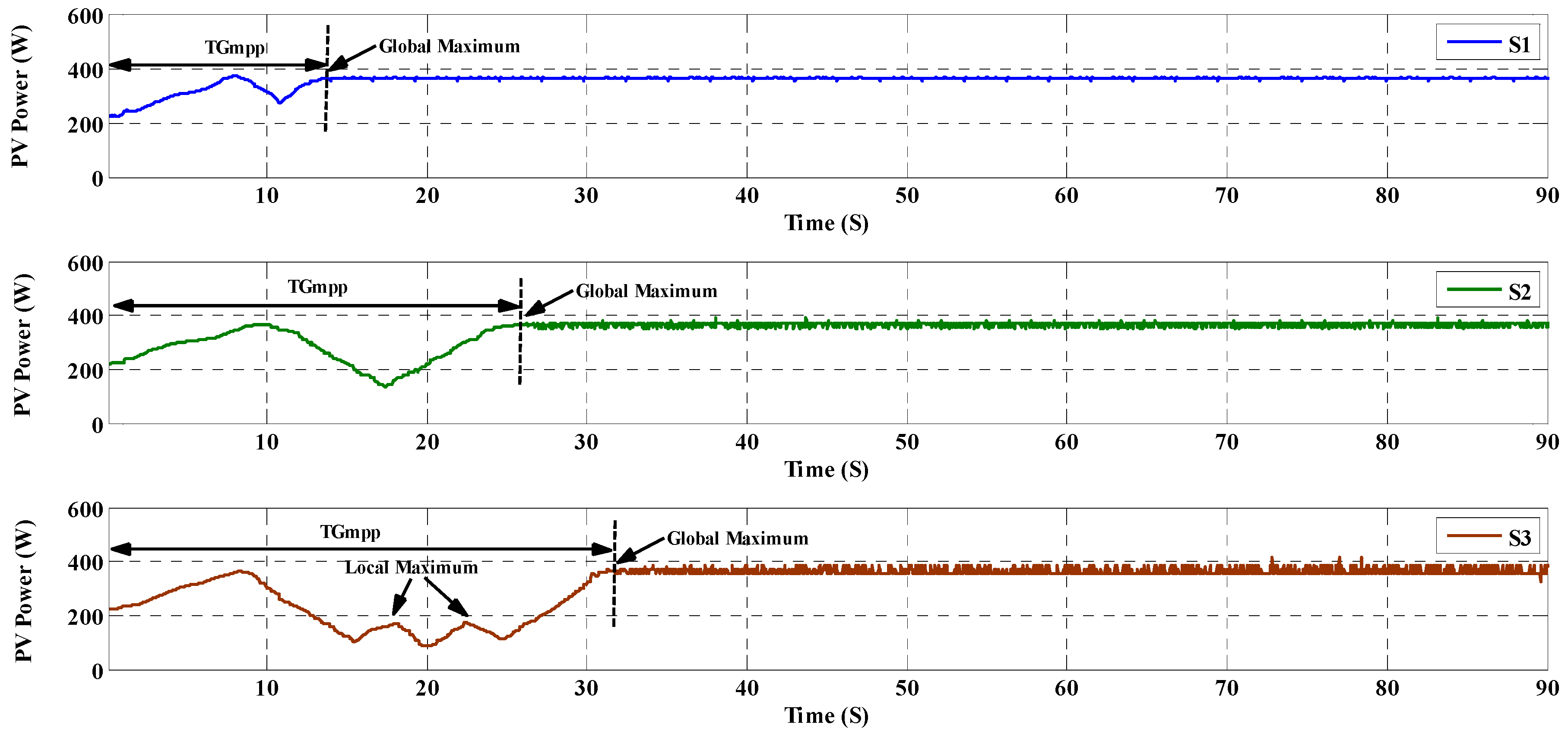
- TGMPP: The global maximum power point reaching time (s);
- Pave_uni: The average maximum power point value in uniform condition (W);
- Pave_PSC: The average maximum power point value under PSC (W);
- Pripp_uni: The oscillation in power in uniform condition (W);
- Pripp_PSC: The oscillation in power under PSC (W).
| Items | Scenario | SOP | TGMPP | Pave_uni | Pave_PSC | Pripp_uni | Pripp_PSC | |
|---|---|---|---|---|---|---|---|---|
| System | ||||||||
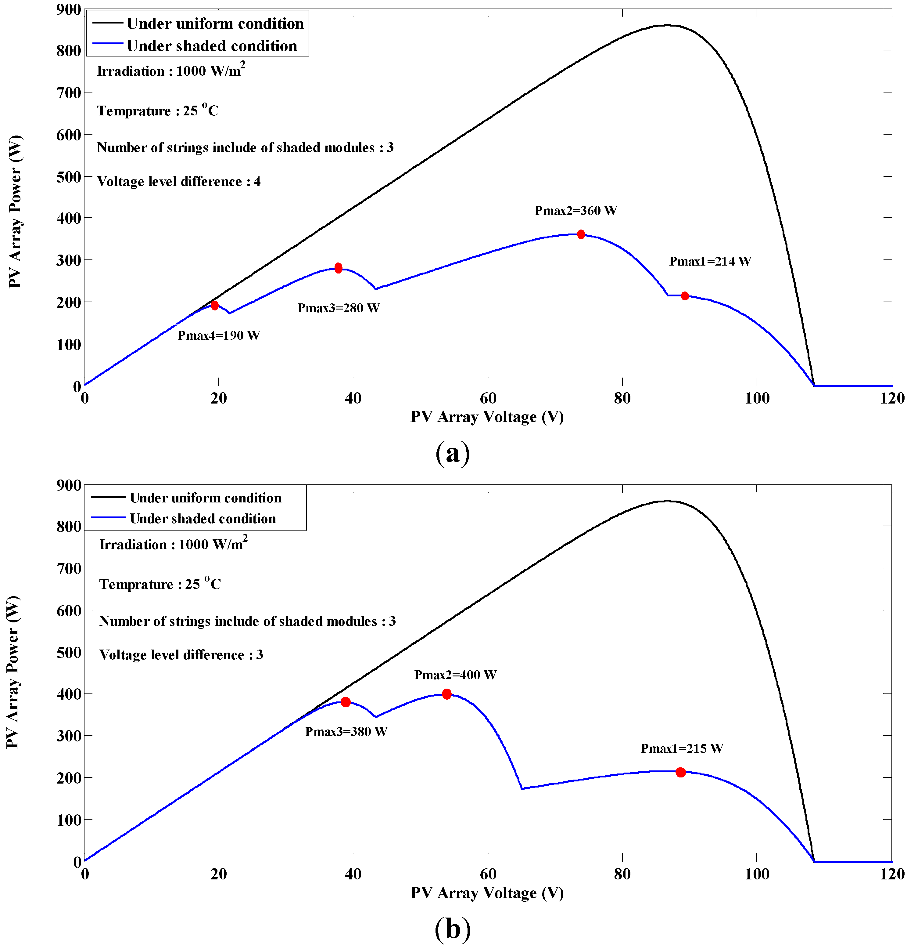
| S1 | 12a | Successful | 0.07 | 860 | 359.5 | 0.3 | 1 | |
| S2 | 12a | Failed | - | 858 | - | 5 | - | |
| S3 | 12a | Successful | 0.074 | 855 | 358 | 9 | 4 | |
| S1 | 12b | Successful | 0.0545 | 860 | 398 | 0.3 | 0.1 | |
| S2 | 12b | Failed | - | 858 | - | 5 | - | |
| S3 | 12b | Successful | 0.0563 | 855 | 397 | 9 | 1.5 | |


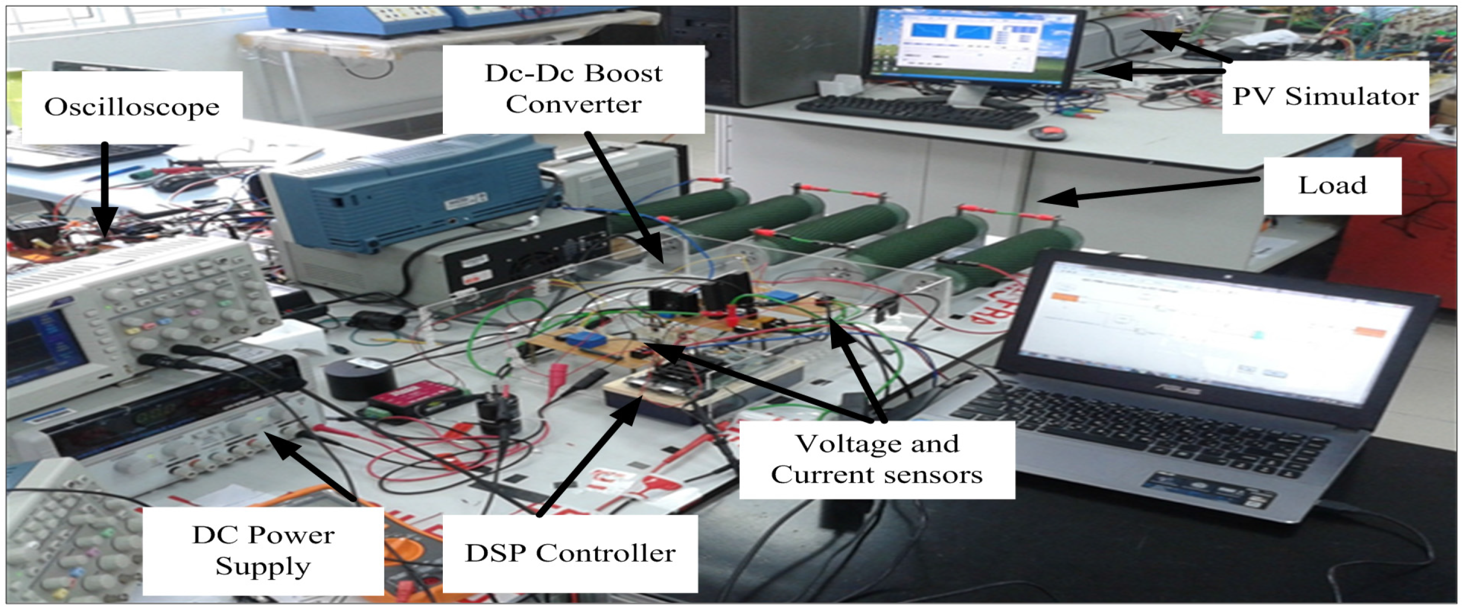
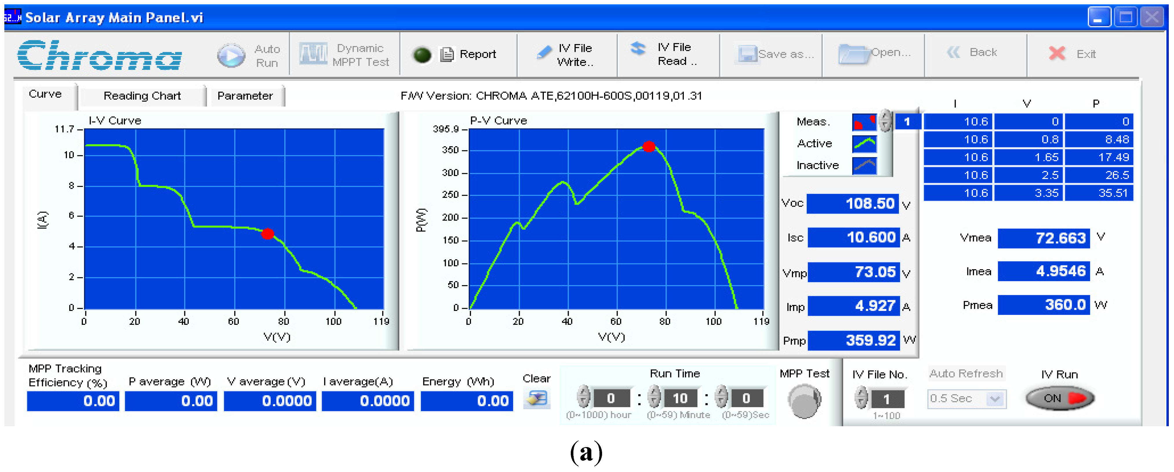
7. Hardware Implementation


| Items | Scenario | SOP | TGMPP | Pave_PSC | Pripp_PSC | |
|---|---|---|---|---|---|---|
| System | ||||||
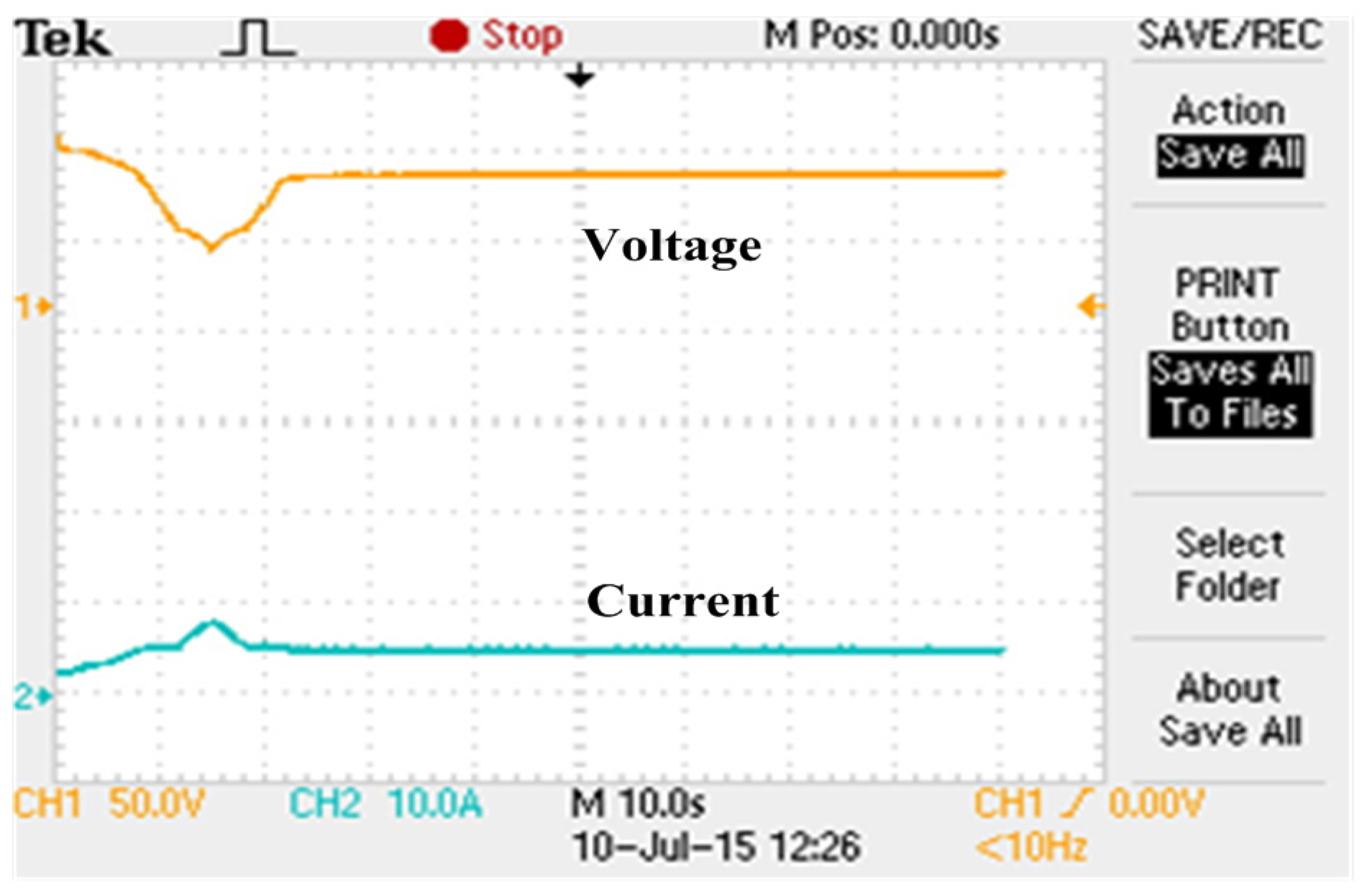
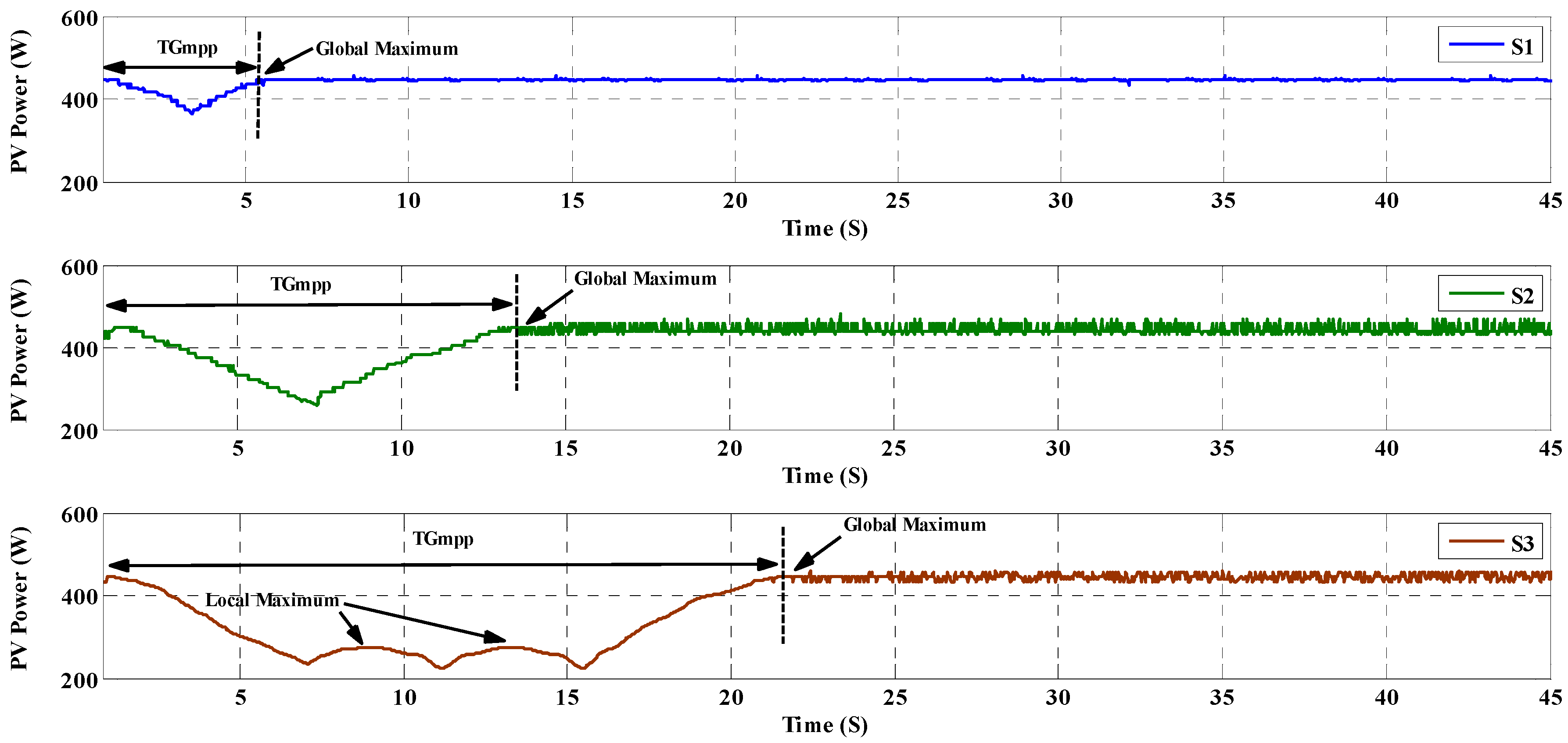
| S1 | 16 | Successful | 22.64 | 360 | 4.5 | |
| S2 | 16 | Failed | - | 278.8 | - | |
| S3 | 16 | Successful | 24.68 | 360 | 11.6 | |
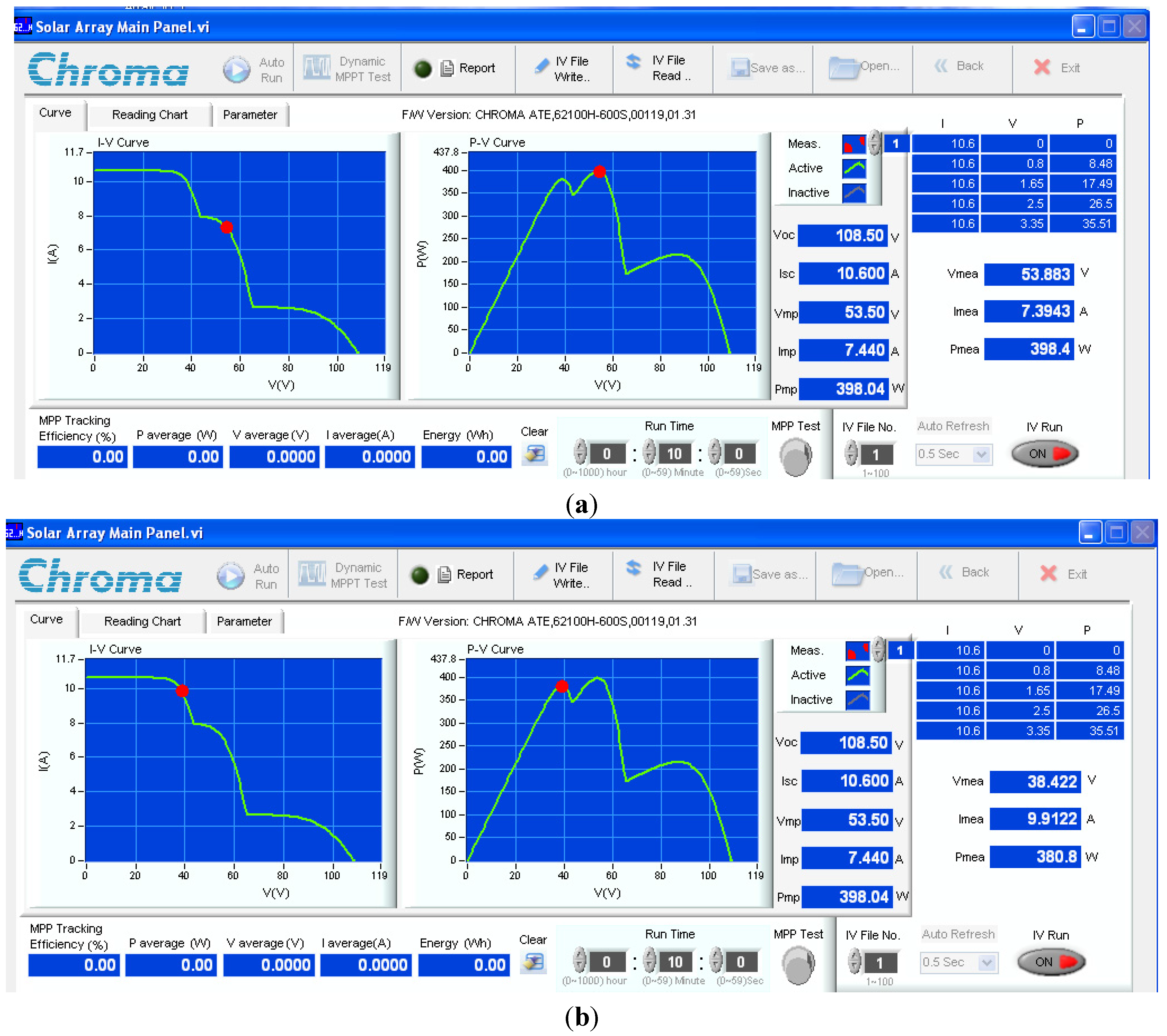
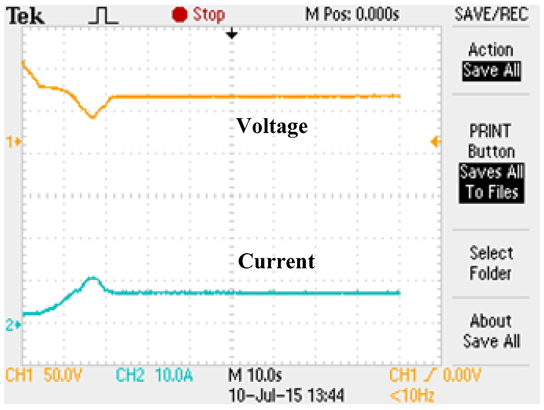
| S1 | 19 | Successful | 20.76 | 398.4 | 3.8 | |
| S2 | 19 | Failed | - | 380.8 | - | |
| S3 | 19 | Successful | 24.08 | 398.4 | 9.6 | |
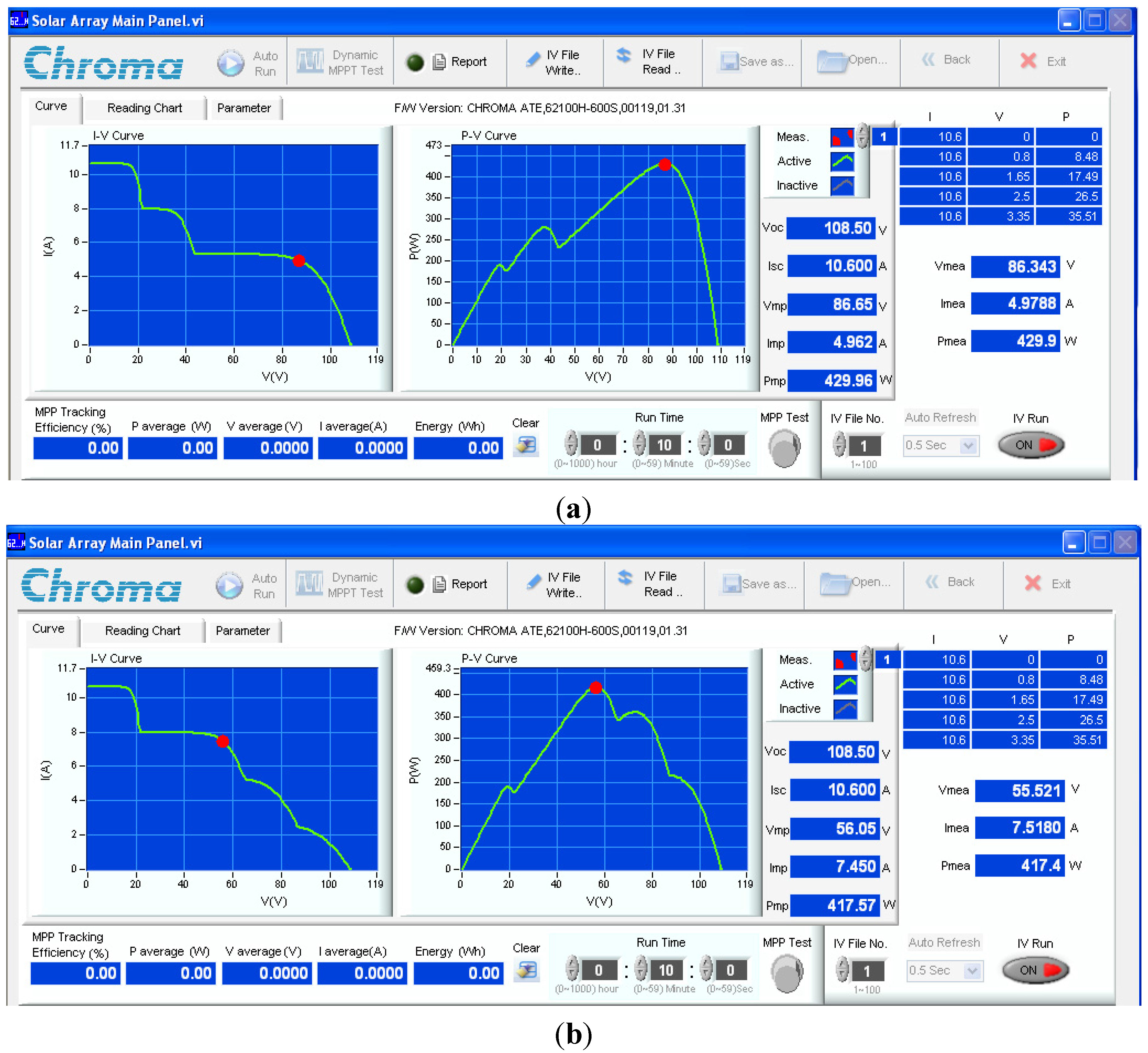
| S1 | 22.a | Successful | 5.2 | 429.9 | 4.5 | |
| S2 | 22.a | Successful | 13.88 | 429.9 | 14.2 | |
| S3 | 22.a | Successful | 21.8 | 429.9 | 12.5 | |
| S1 | 22.b | Successful | 15.72 | 417.4 | 3.2 | |
| S2 | 22.b | Successful | 23.48 | 417.4 | 10.3 | |
| S3 | 22.b | Successful | 27.24 | 417.4 | 11.1 | |
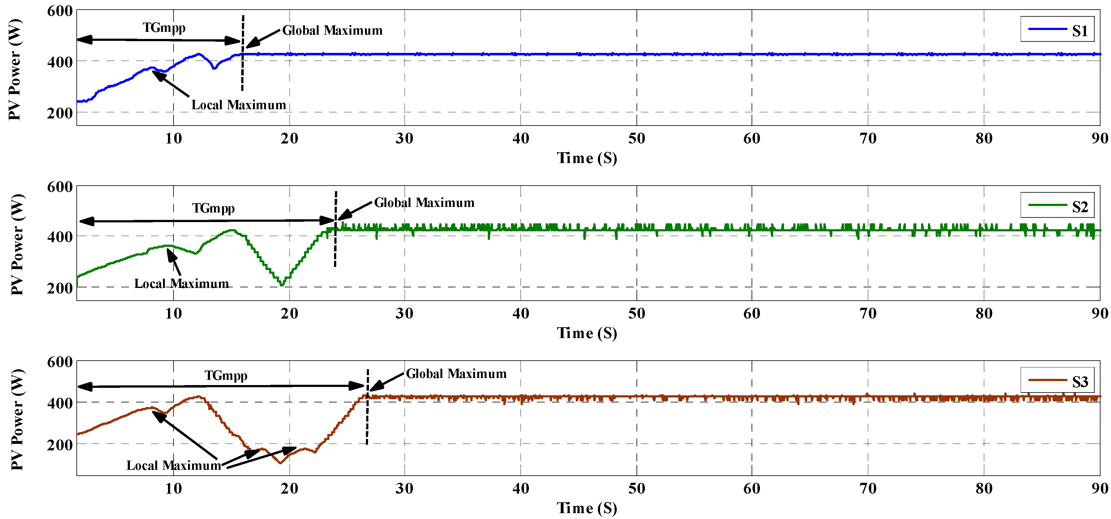
| S1 | 26 | Successful | 13.48 | 359.6 | 2.8 | |
| S2 | 26 | Successful | 25.48 | 359.6 | 9.2 | |
| S3 | 26 | Successful | 31.4 | 359.6 | 10.4 | |
8. Conclusions
Acknowledgments
Author Contributions
Conflicts of Interest
References
- Tomabechi, K. Energy resources in the future. Energies 2010, 3, 686–695. [Google Scholar] [CrossRef]
- Liu, G.; Nguang, S.K.; Partridge, A. A general modeling method for I–V characteristics of geometrically and electrically configured photovoltaic arrays. Energy Convers. Manag. 2011, 52, 3439–3445. [Google Scholar] [CrossRef]
- Shirzadi, S.; Hizam, H.; Wahab, N.I.A. Mismatch losses minimization in photovoltaic arrays by arranging modules applying a genetic algorithm. Sol. Energy 2014, 108, 467–478. [Google Scholar] [CrossRef]
- Elminir, H.K.; Ghitas, A.E.; Hamid, R.; El-Hussainy, F.; Beheary, M.; Abdel-Moneim, K.M. Effect of dust on the transparent cover of solar collectors. Energy Convers. Manag. 2006, 47, 3192–3203. [Google Scholar] [CrossRef]
- Ishaque, K.; Salam, Z. A review of maximum power point tracking techniques of PV system for uniform insolation and partial shading condition. Renew. Sustain. Energy Rev. 2013, 19, 475–488. [Google Scholar] [CrossRef]
- Piegari, L.; Rizzo, R.; Spina, I.; Tricoli, P. Optimized adaptive perturb and observe maximum power point tracking control for photovoltaic generation. Energies 2015, 8, 3418–3436. [Google Scholar] [CrossRef]
- Lee, J.-S.; Lee, K.B. Variable dc-link voltage algorithm with a wide range of maximum power point tracking for a two-string PV system. Energies 2013, 6, 58–78. [Google Scholar] [CrossRef]
- Yau, H.-T.; Wu, C.-H. Comparison of extremum-seeking control techniques for maximum power point tracking in photovoltaic systems. Energies 2011, 4, 2180–2195. [Google Scholar] [CrossRef]
- Sera, D.; Kerekes, T.; Teodorescu, R.; Blaabjerg, F. Improved MPPT algorithms for rapidly changing environmental conditions. In Proceedings of the 12th International Power Electronics and Motion Control Conference (EPE-PEMC), Portoroz, Slovenia, 30 August–1 September 2006; pp. 1614–1619.
- Pilawa-Podgurski, R.C.; Perreault, D.J. Submodule integrated distributed maximum power point tracking for solar photovoltaic applications. IEEE Trans. Power Electron. 2013, 28, 2957–2967. [Google Scholar] [CrossRef]
- Boztepe, M.; Guinjoan, F.; Velasco-Quesada, G.; Silvestre, S.; Chouder, A.; Karatepe, E. Global MPPT scheme for photovoltaic string inverters based on restricted voltage window search algorithm. IEEE Trans. Ind. Electron. 2014, 61, 3302–3312. [Google Scholar] [CrossRef]
- Bazzi, A.M.; Krein, P.T. Ripple correlation control: an extremum seeking control perspective for real-time optimization. IEEE Trans. Power Electron. 2014, 29, 988–995. [Google Scholar] [CrossRef]
- Shiau, J.-K.; Wei, Y.-C.; Lee, M.-Y. Fuzzy controller for a voltage-regulated solar-powered MPPT system for hybrid power system applications. Energies 2015, 8, 3292–3312. [Google Scholar] [CrossRef]
- El Khateb, A.H.; Rahim, N.A.; Selvaraj, J. Fuzzy logic control approach of a maximum power point employing SEPIC converter for standalone photovoltaic system. Procedia Environ. Sci. 2013, 17, 529–536. [Google Scholar] [CrossRef]
- Hajighorbani, S.; Radzi, M.; Kadir, M.A.; Shafie, S.; Khanaki, R.; Maghami, M. Evaluation of fuzzy logic subsets effects on maximum power point tracking for photovoltaic system. Int. J. Photoenergy 2014, 2014, 719126. [Google Scholar] [CrossRef]
- Guenounou, O.; Dahhou, B.; Chabour, F. Adaptive fuzzy controller based MPPT for photovoltaic systems. Energy Convers. Manag. 2014, 78, 843–850. [Google Scholar] [CrossRef]
- Liu, C.-L.; Chen, J.-H.; Liu, Y.-H.; Yang, Z.-Z. An asymmetrical fuzzy-logic-control-based MPPT algorithm for photovoltaic systems. Energies 2014, 7, 2177–2193. [Google Scholar] [CrossRef]
- Hiyama, T.; Kitabayashi, K. Neural network based estimation of maximum power generation from PV module using environmental information. IEEE Trans. Energy Convers. 1997, 12, 241–247. [Google Scholar] [CrossRef]
- Muthuramalingam, M.; Manoharan, P. Comparative analysis of distributed MPPT controllers for partially shaded stand alone photovoltaic systems. Energy Convers. Manag. 2014, 86, 286–299. [Google Scholar] [CrossRef]
- Chowdhury, S.R.; Saha, H. Maximum power point tracking of partially shaded solar photovoltaic arrays. Sol. Energy Mater. Sol. Cells 2010, 94, 1441–1447. [Google Scholar] [CrossRef]
- Jiang, L.L.; Maskell, D.L.; Patra, J.C. A novel ant colony optimization-based maximum power point tracking for photovoltaic systems under partially shaded conditions. Energy Build. 2013, 58, 227–236. [Google Scholar] [CrossRef]
- Shaiek, Y.; Smida, M.B.; Sakly, A.; Mimouni, M.F. Comparison between conventional methods and GA approach for maximum power point tracking of shaded solar PV generators. Sol. Energy 2013, 90, 107–122. [Google Scholar] [CrossRef]
- Sarvi, M.; Ahmadi, S.; Abdi, S. A PSO-based maximum power point tracking for photovoltaic systems under environmental and partially shaded conditions. Prog. Photovolt. Res. Appl. 2015, 23, 201–214. [Google Scholar] [CrossRef]
- Zbeeb, A.; Devabhaktuni, V.; Sebak, A.R. Improved photovoltaic MPPT algorithm adapted for unstable atmospheric conditions and partial shading. In Proceedings of the 2009 International Conference on Clean Electrical Power, Capri, Italy, 9–11 June 2009; pp. 320–323.
- Levron, Y.; Shmilovitz, D. Maximum power point tracking employing sliding mode control. IEEE Trans. Circuits Syst. I Regul. Papers 2013, 60, 724–732. [Google Scholar] [CrossRef]
- Cabal, C.; Martínez-Salamero, L.; Séguier, L.; Alonso, C.; Guinjoan, F. Maximum power point tracking based on sliding-mode control for output-series connected converters in photovoltaic systems. IET Power Electron. 2013, 7, 914–923. [Google Scholar] [CrossRef]
- Ishaque, K.; Salam, Z.; Taheri, H.; Shamsudin, A. maximum power point tracking for PV System under partial shading condition via particle swarm optimization. In Proceedings of the IEEE Applied Power Electronics Colloquium (IAPEC), Johor Bahru, Malaysia, 18–19 April 2011.
- Tsai, M.-F.; Tseng, C.-S.; Hong, G.-D.; Lin, S.-H. A novel MPPT control design for PV modules using neural network compensator. In Proceedings of the 2012 IEEE International Symposium on Industrial Electronics (ISIE), Hangzhou, China, 28–31 May 2012; pp. 1742–1747.
- Jiang, L.L.; Nayanasiri, D.; Maskell, D.L.; Vilathgamuwa, D. A Simple and efficient hybrid maximum power point tracking method for PV systems under partially shaded condition. In Proceedings of the IECON 39th Annual Conference of the IEEE Industrial Electronics Society, Vienna, Austria, 10–13 November 2013; pp. 1513–1518.
- Lian, K.; Jhang, J.; Tian, I. A maximum power point tracking method based on perturb-and-observe combined with particle swarm optimization. IEEE J. Photovolt. 2014, 4, 626–633. [Google Scholar] [CrossRef]
- Kobayashi, K.; Takano, I.; Sawada, Y. A study of a two stage maximum power point tracking control of a photovoltaic system under partially shaded insolation conditions. Sol. Energy Mater. Sol. Cells 2006, 90, 2975–2988. [Google Scholar] [CrossRef]
- Nguyen, D.; Lehman, B. An adaptive solar photovoltaic array using model-based reconfiguration algorithm. IEEE Trans. Ind. Electron. 2008, 55, 2644–2654. [Google Scholar] [CrossRef]
- Patel, H.; Agarwal, V. Maximum power point tracking scheme for PV systems operating under partially shaded conditions. IEEE Trans. Ind. Electron. 2008, 55, 1689–1698. [Google Scholar] [CrossRef]
- Bayod-Rújula, Á.-A.; Cebollero-Abián, J.-A. A novel MPPT method for PV systems with irradiance measurement. Sol. Energy 2014, 109, 95–104. [Google Scholar]
- Radjai, T.; Rahmani, L.; Mekhilef, S.; Gaubert, J.P. Implementation of a modified incremental conductance MPPT algorithm with direct control based on a fuzzy duty cycle change estimator using Dspace. Sol. Energy 2014, 110, 325–337. [Google Scholar] [CrossRef]
- Al-Diab, A.; Sourkounis, C. Variable Step Size P & O MPPT algorithm for PV systems. In Proceedings of the 12th International Conference on Optimization of Electrical and Electronic Equipment (OPTIM), Bochum, Germany, 20–22 May 2010; pp. 1097–1102.
- Mellit, A.; Rezzouk, H.; Messai, A.; Medjahed, B. FPGA-based real time implementation of MPPT-controller for photovoltaic systems. Renew. Energy 2011, 36, 1652–1661. [Google Scholar] [CrossRef]
- Yang, Y.; Zhao, F.P. Adaptive perturb and observe MPPT technique for grid-connected photovoltaic inverters. Procedia Eng. 2011, 23, 468–473. [Google Scholar] [CrossRef]
- Ji, Y.-H.; Jung, D.-Y.; Kim, J.-G.; Kim, J.-H.; Lee, T.-W.; Won, C.-Y. A real maximum power point tracking method for mismatching compensation in PV array under partially shaded conditions. IEEE Trans. Power Electron. 2011, 26, 1001–1009. [Google Scholar] [CrossRef]
- Woyte, A.; Nijs, J.; Belmans, R. Partial shadowing of photovoltaic arrays with different system configurations: Literature review and field test results. Sol. Energy 2003, 74, 217–233. [Google Scholar] [CrossRef]
- Ji, Y.-H.; Kim, J.-G.; Park, S.-H.; Kim, J.-H.; Won, C.-Y. C-language based PV array simulation technique considering effects of partial shading. In Proceedings of the IEEE International Conference on Industrial Technology, Gippsland, Australia, 10–13 February 2009; pp. 1–6.
- Gokmen, N.; Karatepe, E.; Ugranli, F.; Silvestre, S. Voltage band based global MPPT controller for photovoltaic systems. Sol. Energy 2013, 98, 322–334. [Google Scholar] [CrossRef]
- Erickson, R.W.; Maksimovic, D. Fundamentals of Power Electronics; Springer-Verlag: Berlin, Germany, 2001. [Google Scholar]
- El Ela, M.A.; Roger, J. Optimization of the function of a photovoltaic array using a feedback control system. Sol. Cells 1984, 13, 107–119. [Google Scholar] [CrossRef]
- Salas, V.; Olias, E.; Barrado, A.; Lazaro, A. Review of the maximum power point tracking algorithms for stand-alone photovoltaic systems. Sol. Energy Mater. Sol. Cells 2006, 90, 1555–1578. [Google Scholar] [CrossRef]
- Oshiro, Y.; Ono, H.; Urasaki, N. A MPPT Control method for stand-alone photovoltaic system in consideration of partial shadow. In Proceedings of the 2011 IEEE Ninth International Conference on Power Electronics and Drive Systems (PEDS), Singapore, 5–8 December 2011; pp. 1010–1014.
- Skoplaki, E.; Palyvos, J. On the temperature dependence of photovoltaic module electrical performance: A review of efficiency/power correlations. Sol. Energy 2009, 83, 614–624. [Google Scholar] [CrossRef]
- Kroposki, B.; Myers, D.; Emery, K.; Mrig, L.; Whitaker, C.; Newmiller, J. Photovoltaic module energy rating methodology development. In Proceedings of the Conference Record of the 25th IEEE Photovoltaic Specialists Conference, Washington, DC, USA, 13–17 May 1996.
© 2015 by the authors; licensee MDPI, Basel, Switzerland. This article is an open access article distributed under the terms and conditions of the Creative Commons Attribution license (http://creativecommons.org/licenses/by/4.0/).
Share and Cite
Hajighorbani, S.; Radzi, M.A.M.; Kadir, M.Z.A.A.; Shafie, S. Dual Search Maximum Power Point (DSMPP) Algorithm Based on Mathematical Analysis under Shaded Conditions. Energies 2015, 8, 12116-12146. https://doi.org/10.3390/en81012116
Hajighorbani S, Radzi MAM, Kadir MZAA, Shafie S. Dual Search Maximum Power Point (DSMPP) Algorithm Based on Mathematical Analysis under Shaded Conditions. Energies. 2015; 8(10):12116-12146. https://doi.org/10.3390/en81012116
Chicago/Turabian StyleHajighorbani, Shahrooz, Mohd Amran Mohd Radzi, Mohd Zainal Abidin Ab Kadir, and Suhaidi Shafie. 2015. "Dual Search Maximum Power Point (DSMPP) Algorithm Based on Mathematical Analysis under Shaded Conditions" Energies 8, no. 10: 12116-12146. https://doi.org/10.3390/en81012116