1. Introduction
The anti-lock braking system (ABS) is the most important active safety system for road vehicles. The ABS can greatly improve the safety of a vehicle in extreme circumstances since the ABS can maximize the longitudinal tire-road friction while keeping large lateral (directional) forces that ensure vehicle drive-ability [
1]. At present, the ABS has become standard equipment for all new passenger cars in many countries.
As a key technology, regenerative braking is an effective approach to improve vehicle efficiency, and has been applied in various types of electric vehicles (EVs). However, the conventional friction braking system must be retained and works together with the regenerative braking system since the regenerative braking torque is limited by many factors, such as the motor speed, the state of charge (
SOC) and temperature of the battery [
2]. This prompts the development and investigation of regenerative braking strategies and control methods during normal braking events and emergency braking events [
3,
4].
Tur
et al. [
5] proposed a method that employed pure regenerative braking force with proportion-integral-differential (PID) control when the ABS works. The simulation results with a quarter vehicle model showed that the regenerative ABS response is better for panic stop situations. Bera
et al. [
6] discussed a bond graph model of a vehicle with the ABS and regenerative braking module, and a sliding mode controller (SMC) for ABS was developed. Based on a motor priority distribution algorithm, the braking force was distributed between the regenerative braking and the antilock braking in emergency/panic braking situations. Simulations showed that with combined regenerative and antilock braking, the vehicle’s safety and energy efficiency both increases. Peng
et al. [
2] put forward a fuzzy logic control (FLC) strategy for a regenerative braking and antiskid braking system for hybrid EVs (HEVs), and the coordinative control between the regenerative and hydraulic braking were developed. Simulation and experimental results showed that vehicle braking performance and fuel economy can be improved and the proposed control strategy and method are effective and robust.
As is well known, the control of the ABS is complicated. The main difficulty arising in the design of the ABS control is the strong nonlinearity and uncertainty. Standard ABS systems for wheeled vehicles equipped with traditional hydraulic actuators mainly use rule-based control logics. In recent years, technological advances in actuators have led to both electro-hydraulic and electro-mechanical braking (EMB) systems, which enable a continuous modulation of the braking torque [
1]. As a device with fast torque response, the advantage of the motor as an actuator has been realized by more and more researchers. A number of advanced control approaches have been proposed for the ABS, such as FLC [
7], neural network [
8], adaptive control [
9], and other intelligent control.
As actuator of anti-skid control, Sakai
et al. [
10] compared the electric motor with the hydraulic brake system, and the advantage of the electric motor as an actuator is clarified by simulations considering the delay of actuator response. Mi
et al. [
11] presented an iterative learning control for the ABS on various road conditions. Only the electric motor in HEVs and EVs propulsion systems was used to achieve antilock braking performance. Through an iterative learning process, the motor torque was optimized to keep the tire slip ratio corresponding to the peak traction coefficient during braking. Zhou
et al. [
12] proposed a coordinated control of regenerative braking and EMB for a parallel HEV (PHEV), and studied antilock braking control of the EMB to maintain safety and stability of the vehicle using sliding-mode control. To reduce the vibrations induced by the controller, FLC was used to adjust the switching gain of sliding-mode control. Simulation results indicated that the fuzzy-sliding mode control can keep the real slip ratio following the optimal slip ratio closely and quickly.
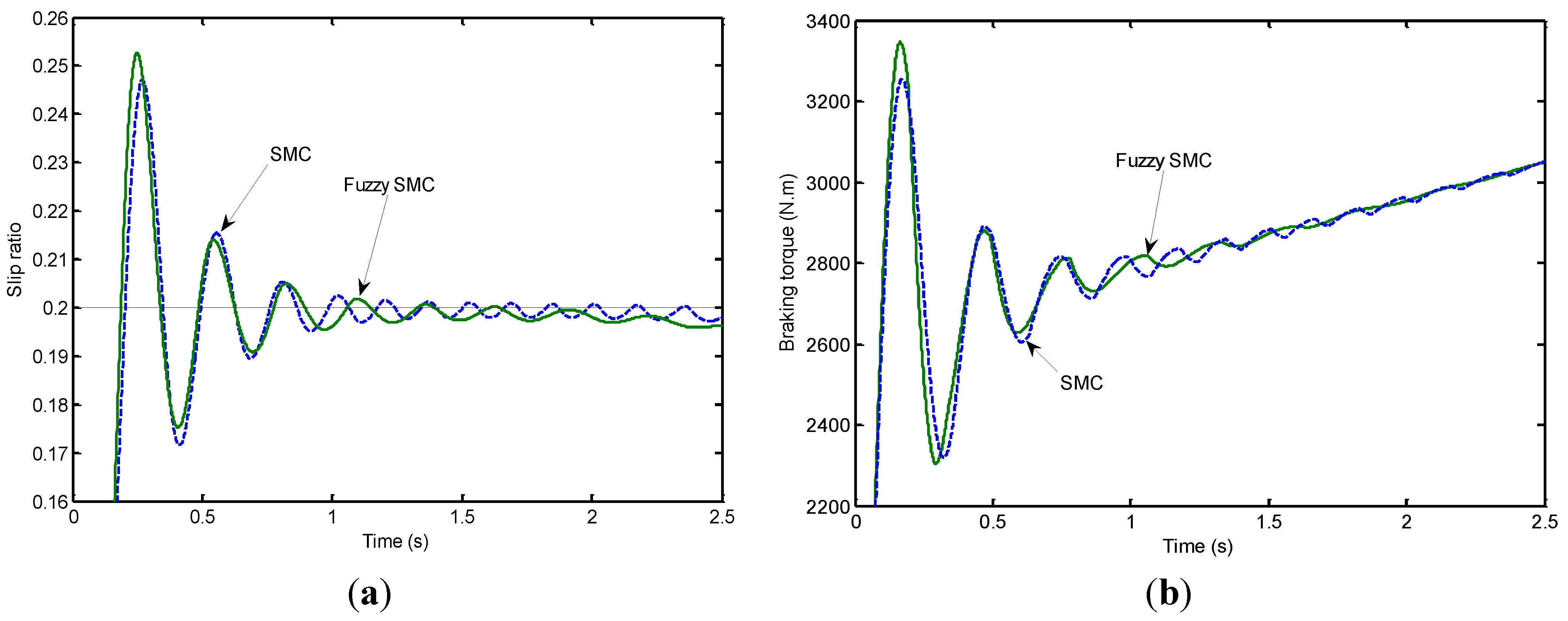
SMC is a variable structure control. SMC has been popularized in many fields for its robust performance against time-dependent parameter variations, disturbances, and simplicity of physical realization [
13]. This is very suitable for ABS control. In this paper, a sliding-mode methodology has been adopted to design the ABS control of a front drive EV. For the drawback of high-frequency chattering generated by the conventional sliding mode control, a method of parameter fuzzy optimization for exponential approach law is proposed, which can meet the requirements for small chattering, strong disturbance attenuation and fast convergence. To maximize the use of the regenerative brake torque, the algorithm of braking force distribution keeps the hydraulic friction brake torque to its minimum. Simulation results show the validity and the effectiveness of the fuzzy SMC. The contribution of the paper includes three aspects: (a) a sliding-mode methodology based on exponential reaching law has been adopted to design the ABS controller; (b) FLC is applied to optimize the parameter of the exponential reaching law; and (c) a distribution algorithm that the motor torque is taken full advantage is adopted to distribute the braking torque between the motor and the hydraulic braking system.
This paper is organized as follows:
Section 2 describes the structure of the braking system investigated in this paper and system modeling, including the three degrees of freedom (3-DOF) longitudinal vehicle model, the Burckhardt tire model, an experimental motor model and a hydraulic brake system model; in
Section 3, a SMC based on exponential reaching law for ABS is developed and the FLC is adopted to optimize the parameter of the exponential reaching law; the regenerative braking algorithm is introduced in
Section 4; then simulations are performed in
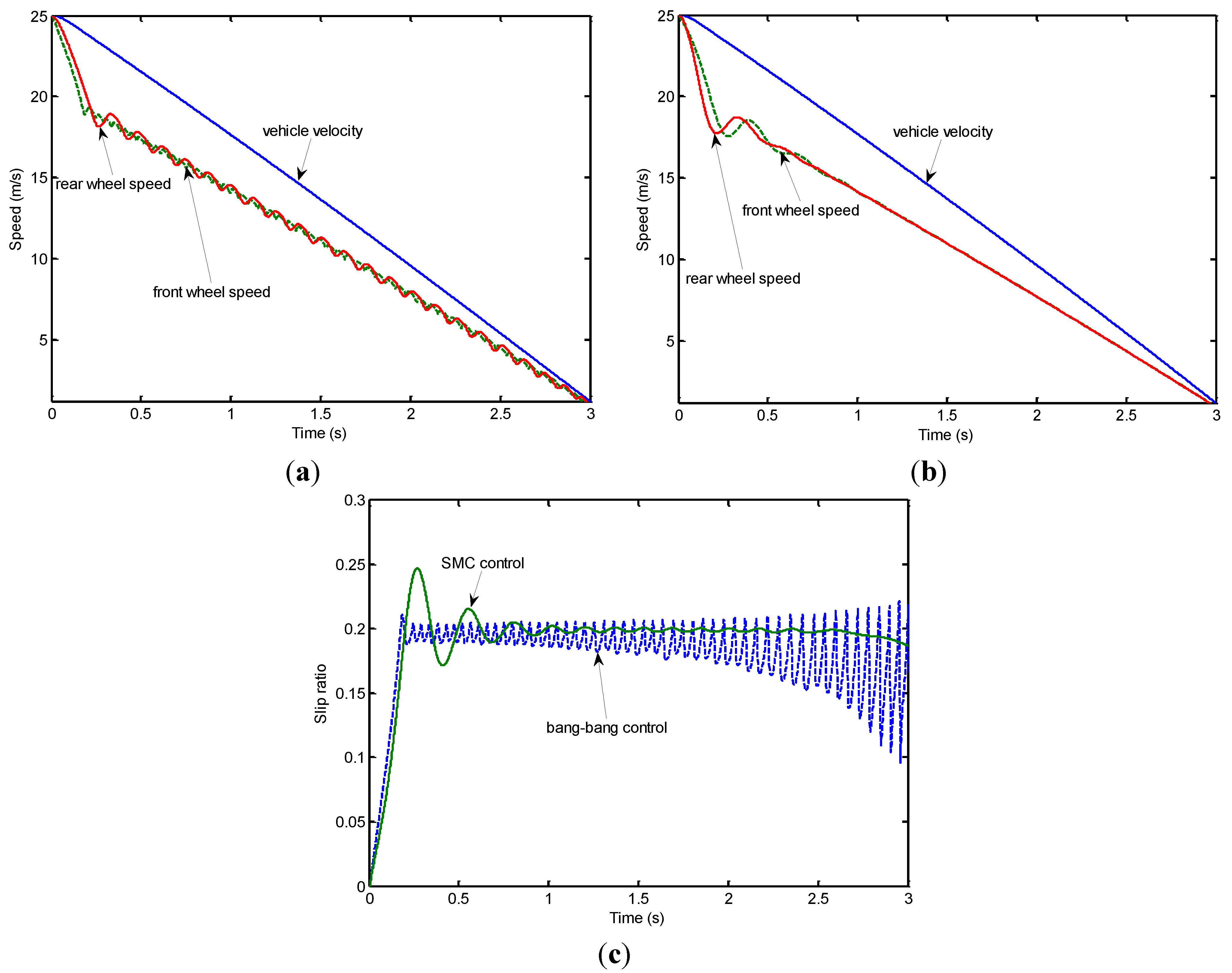
Section 5. The comparisons of performance of ABS with a Bang-bang controller and the proposed SMC controller, with and without the optimizing parameter, and the distribution of braking force using different actuator, are carried out with Matlab/Simulink.
2. System Modeling
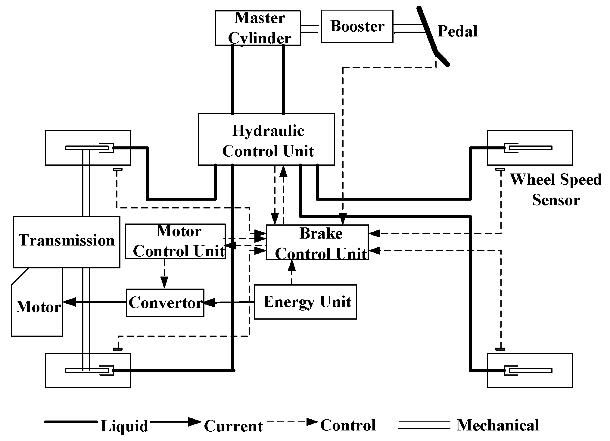
The structure of the braking system investigated in this paper is shown in
Figure 1. The vehicle is considered to have front wheel drive. The motor braking torque is applied to the front wheel through the transmission. The hydraulic brake system consists of a brake pedal, a vacuum booster, a master cylinder, a hydraulic control unit and four wheel cylinders and wheel speed sensors. Wheel speed sensors are mounted on the wheels to measure the wheel speeds and send signals to the brake control unit. When the brake is applied, the brake control unit calculates the required braking torque on the front and rear wheels according to the brake pedal stroke, and estimates the available motor braking torque according to vehicle velocity, battery
SOC and other information. On the base of the braking torque distribution algorithm, the demand motor torque is determined, and the brake control unit sends command signals to the motor control unit. The motor control unit controls the motor work or not to meet the demand on the motor torque, and transmits the actual motor braking torque signals to the brake control unit. The friction braking torque applied to the front wheel is determined by the difference of the required braking torque to the front wheel and the actual motor braking torque. Simultaneously, through the vacuum booster, the master cylinder and the proportional valve, the hydraulic pressure supplied by the brake pedal force is transmitted to the rear wheel cylinders, generating braking torque to the rear wheel.
Figure 1.
Configuration of the braking control system.
Figure 1.
Configuration of the braking control system.
2.1. Vehicle Model
In this paper, only straight-line braking is considered. For the testing of braking control algorithm, a simple but effective model known as the 3-DOF longitudinal vehicle model is used. The main feature of this model is that it can describe the load transfer phenomena. The 3-DOF consists of the longitudinal velocity, the front wheel angular speed, and the rear wheel angular speed. It is worth noting that, in addition to the torque exerted by traditional friction braking system, motor braking torque will also be used on the front wheel since a front-drive EV is studied.
During braking, the dynamic equations [
14] are described as:
where
m is the vehicle mass;
is the vehicle velocity;
Fbf and
Fbr are the braking forces of the front and rear axles, respectively;
Fa is the aerodynamic resistance,
Fa =
Cav2 (
Ca is a constant decided by body style) when the wind speed is ignored;
Ff is the rolling resistance;
Jωf and
Jωr are the inertia moment of the front and rear wheels, respectively;
and
are the angular speed of the front and rear wheels, respectively;
R is the radius of the wheel;
Thf and
Thr are the hydraulic braking torque applied on the front wheel and rear wheel;
Tff and
Tfr are the rolling resistance torque on the front wheel and rear wheel; and
Tmf is the motor braking torque on the front wheel.
During braking, considering load transfer from the rear axle to the front axle, the normal loads on the front and rear axles can be expressed as:
where
Fzf and
Fzr are the normal loads on the front and rear axles, respectively;
W is the vehicle weight;
L is the wheelbase;
hg is the height of the center of mass from the ground;
Lf and
Lr are the distance between the front axle and the rear axle to the center of mass, respectively.
The braking force developed on the tire-road interface is determined by the normal load and the braking effort coefficient of road adhesion. The braking force on the front and rear axles are given by:
where μ is the braking effort coefficient of road adhesion.
2.2. Tire Model
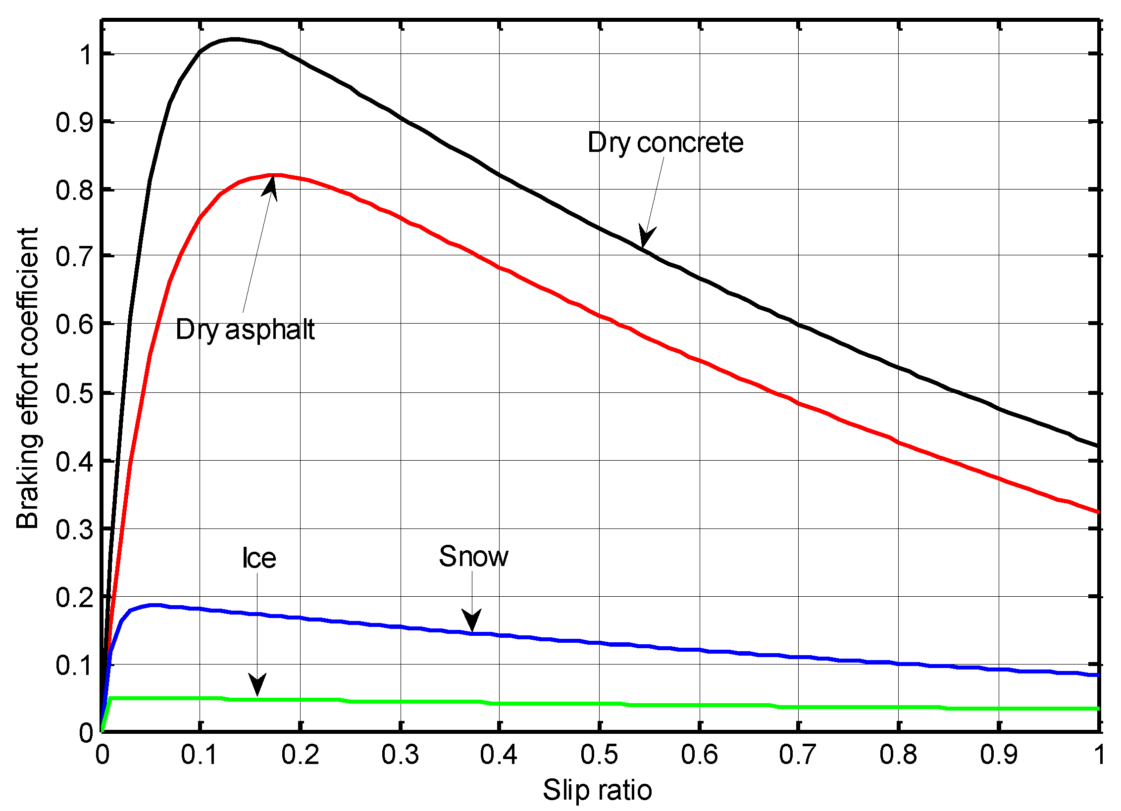
The tire connects the external torques with the vehicle’s longitudinal motion. The tire model includes empirical (semiempirical) and analytical models. Several models describing the nonlinear behavior of the tire have been reported in the literature, such as Magic Formula [
15], LuGre tire model, and so on. In this paper, the Burckhardt model [
16] will be used, as it is particularly suitable for analytical purpose while retaining a good degree of accuracy in the description of the friction coefficient.
During braking, the longitudinal slip ratio is defined as:
where λ is the slip ratio; and ω is the angular speed of the wheel.
Based on Burckhardt model, the velocity dependent braking effort coefficient between the tire and the road has the following form:
where
C1 is the maximum value of friction curve;
C2 is the friction curve shape;
C3 is the friction curve difference between the maximum value and the value at λ = 1; and
C4 is wetness characteristic value. By changing the values of parameters
C1–C4, many different tire-road friction conditions can be modeled. The parameters for different road surfaces are listed in
Table 1.
Table 1.
Tire-road friction parameters.
Table 1.
Tire-road friction parameters.
| Surface conditions | C1 | C2 | C3 | C4 |
|---|
| Dry asphalt | 1.029 | 17.16 | 0.523 | 0.03 |
| Dry concrete | 1.1973 | 25.168 | 0.5373 | 0.03 |
| Snow | 0.1946 | 94.129 | 0.0646 | 0.03 |
| Ice | 0.05 | 306.39 | 0 | 0.03 |
In
Figure 2, the shapes of braking effort coefficient for four different road conditions with a vehicle velocity of 10 m/s are displayed.
When a tire is locked, the braking effort coefficient falls to its sliding value. As a result, the vehicle will lose directional control and stability. The prime function of an antilock brake system is to prevent the tire from locking and ideally to keep the skid of the tire within a desired range.
Figure 2.
Slip-friction curves for different road conditions.
Figure 2.
Slip-friction curves for different road conditions.
2.3. Motor Model
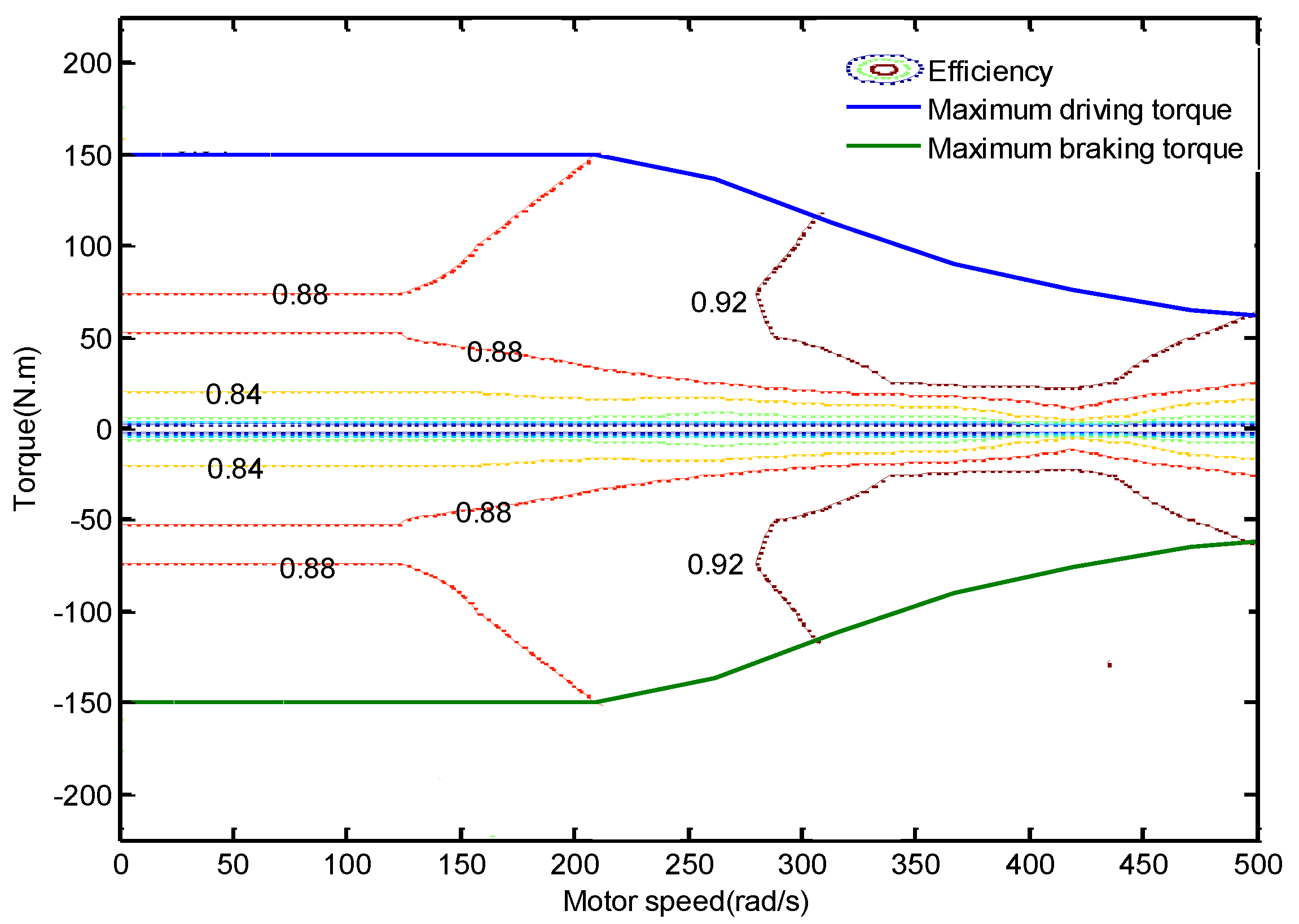
In driving mode, the motor is used as an actuator. However, in the regenerative braking mode, it functions as a generator. The fast torque response characteristics of the motor provide the opportunity to improve the vehicle antilock performance. In this paper, an experimental motor model of a 32 kW permanent magnet synchronous motor from the Advanced Vehicle Simulator (ADVISOR) Database [
17] will be used. The motor model uses lookup table for defining the torque and efficiency characteristics.
Figure 3 shows the maximum torque-speed curve and the efficiency map of the motor at various operating points.
Figure 3.
Motor torque-speed curve and efficiency map.
Figure 3.
Motor torque-speed curve and efficiency map.
During braking, in view of the motor efficiency, the conversion energy by the motor is obtained as:
where
Tm is the motor braking torque;
ωm is the motor angular speed; and
ηreg is the motor efficiency when braking.
As we known, several factors have influence on the regenerative braking torque exerted by the motor. These factors mainly include battery
SOC, motor angular speed and motor temperature [
2]. The impact of motor temperature will be ignored in this paper.
The aim of considering battery
SOC is to protect the battery from overcharging that may affect the battery life. A weight factor
kSOC related to
SOC is introduced and defined as:
The influence of motor angular speed mainly comes from the very low electric motive force (voltage) generated at low motor rotational speed. Similarly, the weight factor
as follow is used:
After the battery
SOC and the motor angular speed are taken into account, the available motor braking torque is obtained as:
where
Tmavail is the available motor braking torque applied at the wheel;
Tmmax is the maximum motor torque, which is related to the motor speed, as shown in
Figure 3;
i is the transmission ratio; and η
t is the transmission efficiency.
When the motor is functioning as an actuator, the motor torque dynamics is very fast compared with hydraulic system. In simulation, the motor torque dynamics is modeled as a first-order system [
10] as:
where
Tm_demand is the demand motor torque; τ
D is the delay constant; and τ
m is the motor torque time constant.
2.4. Hydraulic Brake System
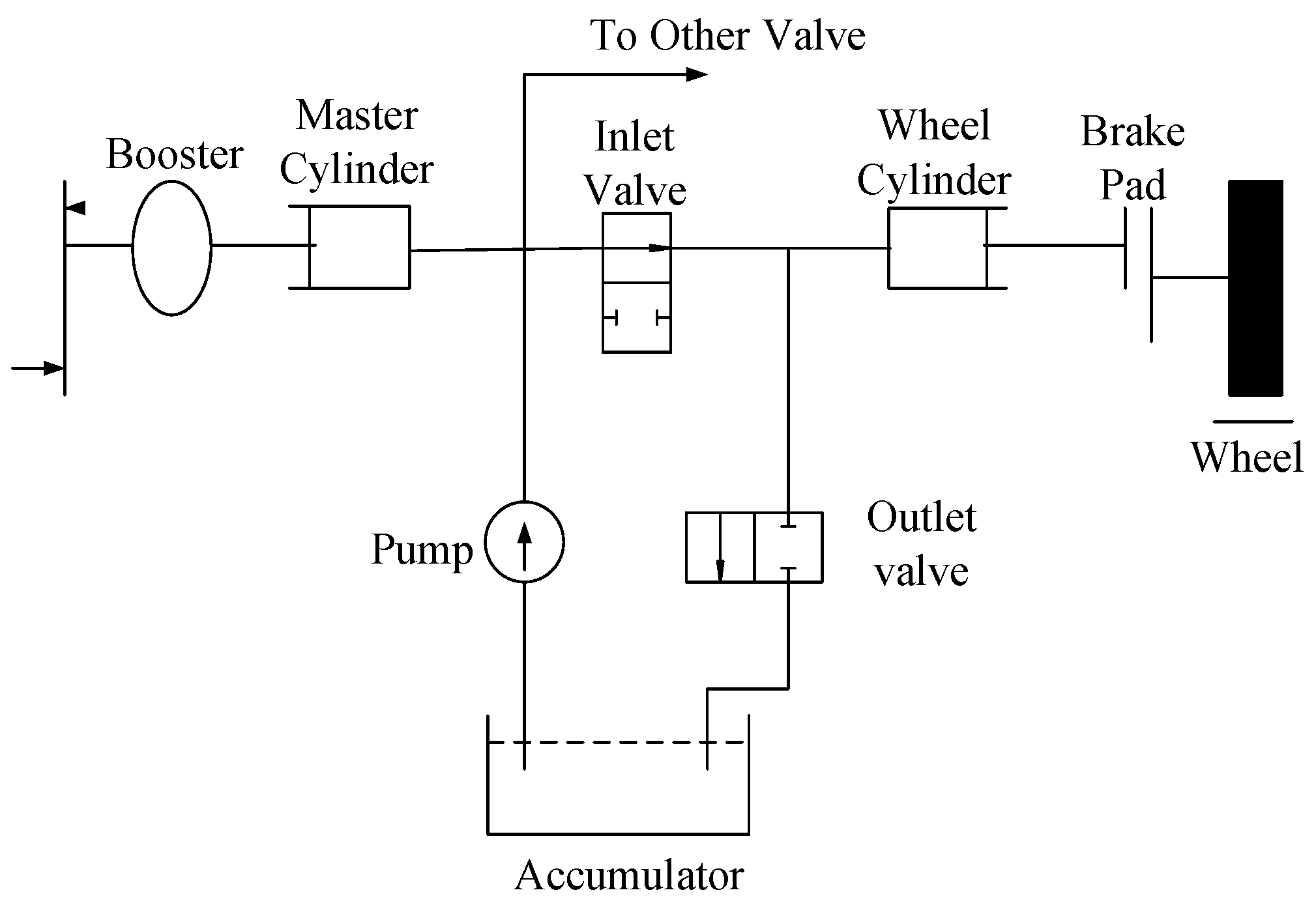
In this paper, a hydraulic brake system as shown in
Figure 4 is used. The braking torque on each wheel depends on the hydraulic pressure of wheel cylinder. In addition, the hydraulic pressure of wheel cylinder can be changed through the coordinative control of the inlet valve and the outlet valve. When the inlet valve is open and the outlet valve is closed, the pressure of wheel cylinder is increasing, and when the inlet valve is closed and the outlet valve is open, the pressure of wheel cylinder will decrease. If the both valves are closed, the brake pressure will be hold. In fact, the operation of an antilock braking system is a constantly switching process of three brake pressure. As can be seen in
Figure 4, the wheel cylinder will necessarily be connected to master cylinder with brake pipes. Therefore, a transport time delay between the demand and the actual brake pressure inevitable exist in the hydraulic line. Of course, the hydraulic circuitry is only one reason that causes the delay, and another reason is the dead time of the solenoid [
10]. There is no doubt that the delay will limit the performance of the actuation. Contrary to the hydraulic brake system, the time response of the motor is quite fast, and the torque control is very precisely, which will improve the vehicle antilock function. The performance of the electric motor with hydraulic brake system as an actuator of antilock brake system is compared in [
10]. Now, the studies on the antilock brake system with the electric motor as actuators are becoming more and more popular.
Figure 4.
Anti-lock braking system (ABS) hydraulic brake system.
Figure 4.
Anti-lock braking system (ABS) hydraulic brake system.
In the next part of this paper, the dynamic model of hydraulic fluid lag of brake system is used as the following first order transfer function:
where
k is the gain of the hydraulic system; and τ is the hydraulic torque time constant.
3. Sliding Mode Controller-Based Anti-Lock Braking System Controller
The objective of the ABS controller is to adjust braking torque so that the wheel slip can track the target slip ratio. In order to improve ABS performance, the control variable must have high frequency of altering. As a variable structure control, sliding mode control is a high-speed switching feedback control that switches between two values based upon some rule, which is suitable for the ABS control.
3.1. Sliding Mode Controller
The sliding mode design approach consists of two components. The first involves designing a sliding surface so that the sliding motion satisfies design specifications. The second is concerned with constructing a switched feedback gains necessary to drive the plant’s state trajectory to the sliding surface. These constructions are built on the generalized Lyapunov stability theory. Note that this control law is not necessarily discontinuous.
Equations (1)–(3) can be rewritten as:
where
i =
f or
r and
j =
f or
r, denoting the variable of front or rear wheel;
Tbi is the braking torque applied by brake system, for the front wheel,
Tbi =
Thf +
Tmf, for the rear wheel,
Tbi =
Thr.
The slip ratio is expressed as:
The differentiation of Equation (16) is:
Inserting Equations (14) and (15) into Equation (17), we can obtain:
As shown in
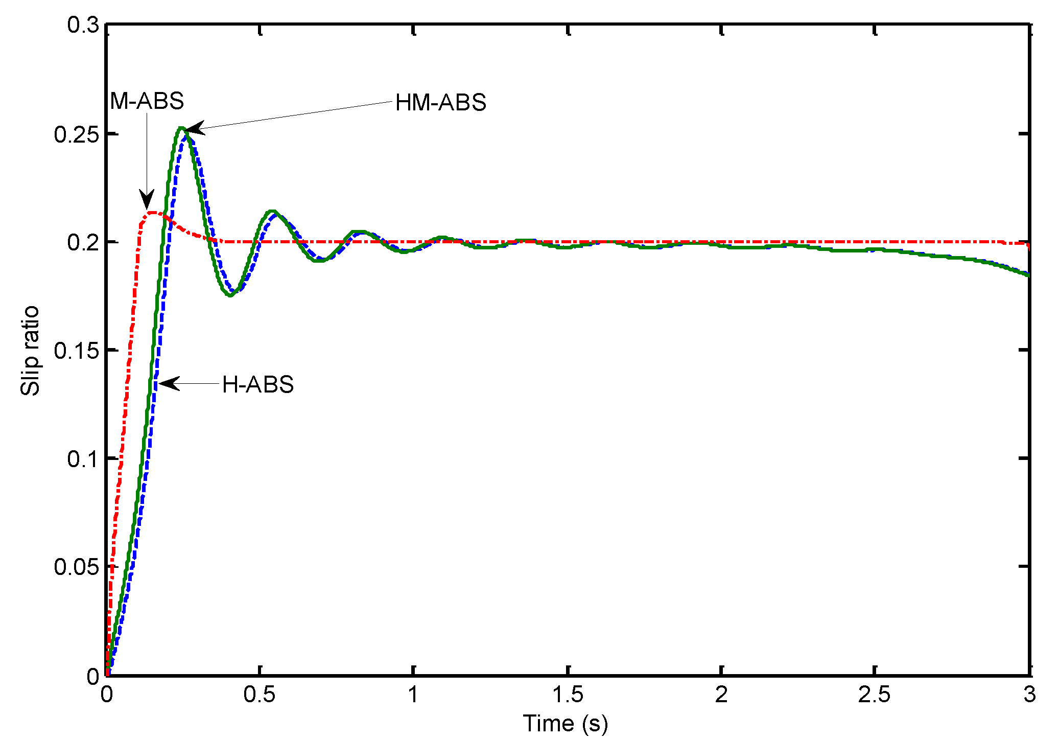
Figure 2, the braking effort coefficient varies significantly depending on the road condition. The goal of the ABS is to take full advantage of the peak braking effort coefficient, which can be achieved by maintaining the slip ratio between 0.15 and 0.25. Although the direct slip ratio measurement is difficult, many researchers have proposed various algorithms about the estimation of the slip ratio [
18,
19].
In order to have the slip ratio λ
i track the desired slip ratio λ
des, the sliding surface will be defined as:
As we know, SMC has good anti-jamming performance. The advantage of SMC is strong robustness, that is to say, it is excellently insensitive to model error and parameters change of controlled object and external disturbance. However, the disadvantage of the SMC is its chattering problem, which is caused by inherent discrete characteristic. Although the chattering can be weakened generally by controlling the speed of state variables close to sliding mode switching plane, the chattering cannot be essentially eliminated. In order to reduce the frequency of the chattering, an exponential approach law is adopted. For a continuous time system, the commonly used exponential approach law is:
where ε and
k are positive constants; and sgn(
S) is a sign function, which is defined as:
Differentiating Equation (19) and substituting Equations (18) and (20) into it result in:
Therefore, the control input
Tbi is obtained as:
If the desired slip ratio λ
des is a constant, then the control law becomes:
It should be noted again, since the motor braking torque is only acted on the front axle, Tbi is the sum of the hydraulic braking torque Thf and the motor braking torque Tmf for the front wheel, and for the rear wheel, Tbi only equals to hydraulic braking torque Thr.
In order to evaluate stability, the following Lyapunov function is selected:
clearly, V > 0.
The differentiation of
V is:
Substituting Equation (18) into above equation gives:
Again, inserting Equation (24) into Equation (27) and simplifying give:
It can be proved, that Equation (28) satisfies the sliding condition
< 0 whenever (λdes – λi) reverses its sign. Therefore, the system is asymptotically stable.
3.2. Parameter Optimizing by Fuzzy Logic Control
For a continuous time system, SMC with exponential reaching law has two adjustable parameters ε and
k. The rational selection of both parameters can ensure rapidly reaching and chattering control. The parameter ε is a factor representing the robustness of the system against the disturbance. The larger the parameter ε is, the stronger robustness of the system is. However, the larger parameter ε will also cause severe chatting phenomenon at the same time. Therefore, a suitable choice of parameter set becomes crucial. In this paper, FLC will be used to determine the parameter ε of exponential approach law [
20].
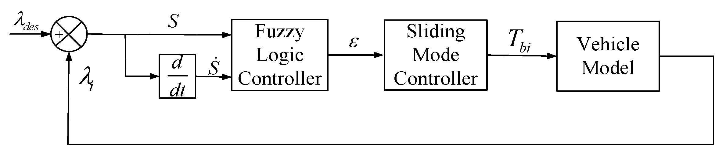
A Mamdani fuzzy logic controller with two inputs and one output is designed. The two inputs are the sliding mode function
S and the differentiation of the sliding mode function
, and the output is the parameter ε of exponential approach law.
Figure 5 shows the principle of the fuzzy sliding mode controller.
Figure 5.
Principle of the fuzzy sliding mode controller (SMC).
Figure 5.
Principle of the fuzzy sliding mode controller (SMC).
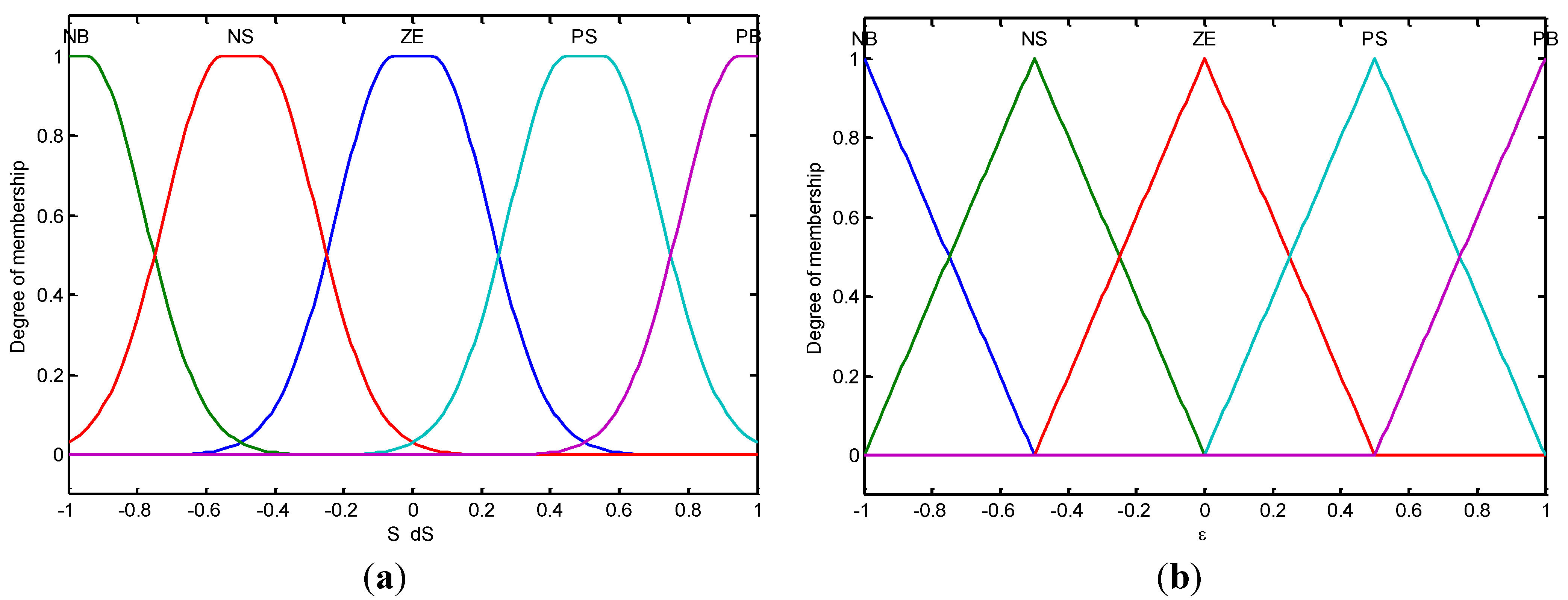
Since 0 ≤ λ
des,λ
i ≤ 1 and
S = (λ
des – λ
i), the domain of the input
S will be [−1,1]. In addition, based on the simulation analysis, the domains of the input
and the output ε are also set as [−1,1]. The inputs and output are all divided into five fuzzy subsets: [NB, NS, ZE, PS, PB], where NB, NS, ZE, PM and PB mean negative big, negative small, zero, positive small and positive big, respectively. Gaussian and triangular shapes are selected for the membership functions of the inputs and the output, as shown in
Figure 6.
Figure 6.
Membership functions for the: (a) inputs and (b) outputs.
Figure 6.
Membership functions for the: (a) inputs and (b) outputs.
Fuzzy rules have the following form: if
S is
Ai and
is
Bi, then ε is
Ci, where
Ai,
Bi and
Ci are linguistic variables. The fuzzy rules are listed in
Table 2.
Table 2.
Rules of the fuzzy logic controller. NB, NS, ZE, PM and PB mean negative big, negative small, zero, positive small and positive big, respectively.
Table 2.
Rules of the fuzzy logic controller. NB, NS, ZE, PM and PB mean negative big, negative small, zero, positive small and positive big, respectively.
| ε | S |
|---|
| NB | NS | ZE | PS | PB |
|---|
| S | NB | NB | NB | NS | ZE | ZE |
| NS | NB | NS | ZE | ZE | ZE |
| ZE | NS | ZE | ZE | ZE | ZE |
| PS | NS | ZE | ZE | PS | PS |
| PB | ZE | ZE | PS | PB | PB |
Defuzzification of the output is accomplished by the gravity center defuzzifier:
where
ki is the weight of the
ith rule; and
n is the number of rules.
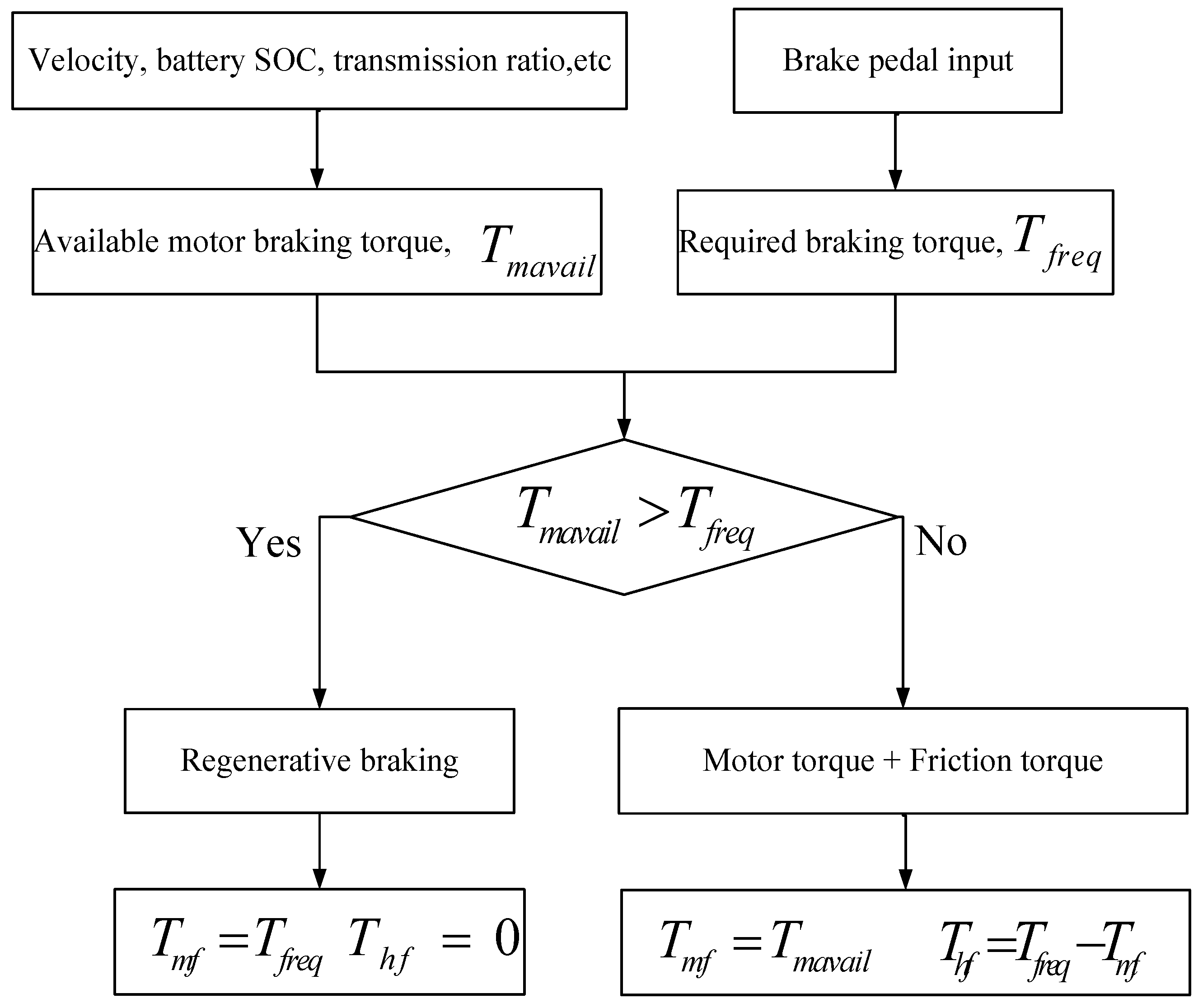
4. Regenerative Braking Algorithm
As stated in
Section 2.3, the motor braking torque is limited by several factors. Therefore, regenerative braking must be carried out together with the friction braking in EVs. For the brake system of EVs, an algorithm is required to decide on how to distribute the braking force between regenerative braking and friction braking in normal braking or emergency braking situations.
As an actuator of braking, the motor not only can convert the braking energy, but also has rapid and precise torque response, which is crucial for ABS. Therefore, from the viewpoints of increasing energy utilization efficiency and improving ABS performance, the motor braking torque should be used to the full extent.
Based on the above goals, for the front wheel, the regenerative braking algorithm shown in
Figure 7 is adopted. During emergency braking, on the one hand, the required braking torque is calculated according to Equation (23) or (24); on the other hand, the available motor braking torque is decided depending on various input parameters as illustrated in
Section 2.3. If the available motor braking torque
Tmavail is less than the required braking torque
Tfreq, then both the motor and friction brake system will work in union. The motor braking torque will be used to its maximum level. The difference between the required braking torque and the actual motor torque will be provided by friction brake system. If the available motor braking torque
Tmavail is more than the required braking torque, then only motor brake will carry out the job, and the motor controller regulates the current input to ensure the required braking torque.
Figure 7.
Flow diagram of regenerative braking. SOC: state of charge.
Figure 7.
Flow diagram of regenerative braking. SOC: state of charge.
For the rear wheel, the required braking torque Trreq will be carried out by friction brake system only. The hydraulic brake controller regulates the wheel cylinder pressure so that the required braking torque is fulfilled.


