Article

A Novel Supercapacitor Model Parameters Identification Method Using Metaheuristic Gradient-Based Optimization Algorithms

1
Mechatronics Graduate Program, College of Engineering, American University of Sharjah, Sharjah 26666, United Arab Emirates
2
Department of Electrical Engineering, College of Engineering, American University of Sharjah, Sharjah 26666, United Arab Emirates
3
Electrical & Computer Engineering and Computer Science Department, University of New Haven, West Haven, CT 06516, USA
*
Author to whom correspondence should be addressed.
Energies 2024, 17(6), 1500; https://doi.org/10.3390/en17061500
Submission received: 20 January 2024 / Revised: 6 March 2024 / Accepted: 9 March 2024 / Published: 21 March 2024

Abstract

:
This paper addresses the critical role of supercapacitors as energy storage systems with a specific focus on their modeling and identification. The lack of a standardized and efficient method for identifying supercapacitor parameters has a definite effect on widespread adoption of supercapacitors, especially in high-power density applications like electric vehicle regenerative braking. The study focuses on parameterizing the Zubieta model for supercapacitors, which involves identifying seven parameters using a hybrid metaheuristic gradient-based optimization (MGBO) approach. The effectiveness of the MGBO method is compared to the existing particle swarm optimization (PSO) and to the following algorithms proposed and developed in this work: ‘modified MGBO’ (M-MGBO) and two PSO variations—one combining PSO and M-MGBO and the other incorporating a local escaping operator (LCEO) with PSO. Metaheuristic- and gradient-based algorithms are both affected by problems associated with locally optimal results and with issues related to enforcing constraints/boundaries on solution values. This work develops the above-mentioned innovations to the MGBO and PSO algorithms for addressing such issues. Rigorous experimentation considering various types of input excitation provides results indicating that hybrid PSO-MGBO and PSO-LCEO outperform traditional PSO, showing improvements of 51% and 94%, respectively, while remaining comparable to M-MGBO. These hybrid approaches effectively estimate Zubieta model parameters. The findings highlight the potential of hybrid optimization strategies in enhancing precision and effectiveness in supercapacitor model parameterization.

1. Introduction

Recently, there has been a noteworthy global upswing in the adoption of renewable energy sources. This increased interest is a proactive response to economic, political, and social factors, all directed toward diminishing dependence on conventional fossil fuels [1,2]. The efficiency of power systems that encompass a substantial share of renewable energy sources is shaped by various factors. Challenges arise from the inherent unpredictability associated with renewable energy sources. Consequently, the use of energy storage systems plays a pivotal role in effectively bringing renewable energy systems into commercial viability [3].
In recent years, there has been a marked uptick in interest surrounding supercapacitors (SCs). They are being viewed as a viable supplementary power source owing to their outstanding high power density and relatively high energy density [4]. The successful incorporation of supercapacitors into energy storage systems has been observed across diverse industrial applications, such as electric vehicles and solar energy systems [5,6]. The integration of SCs provides significant advantages in maintaining stability within electrical power systems. This is achieved by augmenting the energy supply derived from batteries and the unpredictable nature of renewable resources.
To optimize the integration of supercapacitors into energy storage systems, it is crucial to establish a precise dynamic representation that effectively represents the static and dynamic properties of supercapacitors. The precise definition and modeling of the system’s characteristics is a vital step in enhancing and managing any energy storage system. SC dynamic modeling is used to identify and characterize electrical and thermal performances, condition diagnostics-monitoring and estimation of state of charge (SOC), state of power (SOP), state of health (SOH), and control mechanism design [7,8,9]. Supercapacitors are modeled based on the characteristics to be monitored, with five key models: equivalent circuit models, electrochemical models, thermal models, fractional order models, and intelligent models [7,10].
Different models have been developed to explain the behavior of supercapacitors; however, the electrical equivalent circuit models are found to be a convenient and common way to simulate the electrical behavior of SCs. To characterize and simulate the electrical behavior of SC, equivalent circuit models utilize parameterized RC networks defined by ODEs. Utilizing electrical models enables the assessment of supercapacitor capacitance, considering its variations with bias voltage, voltage drop, as well as power loss attributed to internal resistance, self-discharge, and leakage current effects. Additionally, these models account for the electric dynamic behavior influenced by ion diffusion [11,12].
Modeling and characterization of supercapacitors have been extensively investigated using electrochemical impedance spectroscopy (EIS) approaches [13,14,15,16] or time response experiments and simulations [17,18,19,20]. Both techniques aim to provide a variety of equivalent circuit representations that are required for characterizing the state of the SC cell in the course of operation. Hence, when analyzing the time domain system, various circuit models have been proposed. Classical models, multi-stage ladder models, and dynamic models are the three categories of equivalent circuit models. In addition, a wide range of nonlinear models have been formulated for supercapacitors, which include fractional order models, as well as methodologies for determining parameters, thereby demonstrating the effectiveness of these models [21,22]. Nevertheless, the procedure of determining parameters for these models sometimes entails multiple stages of linearization and extensive experimental investigation.
Methods such as adaptive filter algorithms, metaheuristic optimization methods, and intelligent artificial intelligence are being deployed in the literature to find the optimum parameters for the different SC equivalent models. The recursive least squares (RLS) method was used to identify the parameters of the classical equivalent circuit model in [23,24,25]. In [25], the authors used a voltage-dependent capacitor in the first branch instead of the constant capacitance capacitor, making it simpler to identify the time-variant parameters. Similarly, in [26], a nonlinear least square method was used to identify the parameters of a supercapacitor model. The authors provided a framework for the branch number selection criteria and order reduction. The total least-squares method was used in [27] to identify the three parameters (C0, KV, and C2) of the reduced two-branch Zubieta model [28]. The first branch resistor, R0, was assumed to be given by the manufacturer, and the second branch resistor, R2, and the leakage resistor, Rlea, were found using the circuit analysis method. The voltage response, input current, and their second- and first-order derivatives were used to define the estimation problem. The derivatives of the electric variables were obtained using filter differentiation.
Moreover, Kalman filters were used to identify supercapacitor dynamic model parameters online [29]. The authors used the extended Kalman filter to automate the estimation of the error bound. The researchers proved that the proposed estimator model can be used to accurately depict the voltage behavior of the SC under various scenarios.
Optimization is still a challenging computational task. Consequently, numerous algorithms have been proposed to address this challenge. Two questions must be answered to ensure the best possible solution to this problem: how to identify global and local optimization and how to preserve such optimization until the end of the search. Swarm intelligence, which includes particle swarm optimization (PSO) [30], the grey wolf optimizer (GWO) [31], whale optimizer [32], ant-lion optimizer (ALO) [33], genetic algorithm (GA) [34], artificial ecosystem-based optimizer (AEO) [35], and many others, evolved as a result of these questions over the last two decades. These metaheuristic algorithms are widely used to solve and optimize various real-world problems. However, few researchers in the field of energy storage have used metaheuristic optimization algorithms as an appealing tool for identifying electrical circuit model parameters.
In 2022, a study by researchers [36] employed a straightforward and reliable methodology, using the bald eagle search (BES) optimization algorithm to identify the parameters of the Zubieta model’s supercapacitor equivalent circuit [20]. The envisaged bald eagle search algorithm mimics bald eagle hunting behavior to demonstrate the consequences of each stage of hunting. The BES approach’s robustness was assessed in comparison to other metaheuristic algorithms for two supercapacitors (SCs) with modules of 470 F and 1500 F. The authors attained an MSSE of 1.32 × 10⁻⁸ for the 1500 F SC when employing the BES. In contrast, the PSO, the most closely related optimizer based on the obtained results, yielded a higher MSSE of 6.69 × 10⁻⁶.
In [37], a similar approach was used with the interior search optimizer (ISA), a notable metaheuristic optimization algorithm proposed by Gandomi [38]. The mean square error (MSE) for parameterization of a 470 F capacitor using the ISA was 0.004487% compared to 0.0310895 for GWO, 0.0045% for GA, and 0.03109% for WA. These findings suggest that the ISA method can be used to optimize the parameters of the Zubieta model, and they are comparable to the genetic algorithm approach.
In [39], a real-time modeling approach based on the weighting bat algorithm (WBA) was proposed. The model was used for parameter identification in the reduced Zubieta model, enabling real-time power management in embedded systems powered by supercapacitors, as well as predicting supercapacitor behavior. The WBA convergence of the fitness function in 50 iterations is comparable to the genetic algorithm with lower computational time, 0.4328% and 0.43815%, respectively.
Furthermore, the study in [40] introduced an electrical model that is based on the optimization of parameters for a passive electrical circuit model. There exist multiple methodologies for the parameter identification of supercapacitor models. These include the analytical method [20], Segmentation Optimization [41], the binary quadratic equation fitting method [42], Universal Adaptive Stabilization and Optimization [11], Particle Swarm Algorithm (PSO) [43], the recursive least-squares method [44], and other alternative techniques.
Over the past few years, there has been a notable influx of research focusing on the development and application of advanced optimizers for parameter identification, particularly in the field of energy storage systems. Metaheuristic algorithms have continued to dominate the landscape of parameter estimation, offering innovative solutions to address challenges associated with accuracy and convergence rates.
One prominent optimizer in recent literature is the Sine Cosine Algorithm (SCA), introduced by Mirjalili et al. [45]. SCA has shown promise in optimizing complex and nonlinear functions, making it suitable for parameter identification tasks. Studies have applied SCA to various energy storage system models, demonstrating its effectiveness in achieving accurate parameter estimates within a reduced computational time.
Another development, as mentioned earlier, is the grey wolf optimizer (GWO), proposed by Mirjalili et al. [31]. GWO draws inspiration from the social hierarchy of grey wolves and has been successfully applied to parameter identification tasks in renewable energy systems. Its ability to strike a balance between exploitation and exploration makes it well-suited for handling complex and high-dimensional optimization problems.
Other noteworthy contributions are the Dandelion Optimization Algorithm [46] used for the parameter estimation of proton exchange membrane fuel cells (PEMFCs) and the Metaheuristic Mountain Gazelle Optimizer for parameter estimation of single- and double-diode photovoltaic cell models [47]. These new optimization strategies demonstrated improved performance compared with traditional algorithms, showcasing the potential of metaheuristic optimization paradigms to address the complexities associated with renewable energy system models.
Nevertheless, the existing literature points out limitations in the application of meta-heuristic optimizers to identify variables in the SCs equivalent electrical circuit model. Additionally, the currently employed algorithms have their own constraints and highlight notable gaps that warrant further investigation. Existing studies often lack a standardized approach, leading to inconsistencies in parameter estimation. Challenges include the absence of a universally accepted model and the need for improved convergence rates and accuracy in optimization algorithms. Moreover, there is a limited exploration of hybrid optimization strategies that could potentially enhance the efficiency of parameter identification for supercapacitors. Addressing these gaps is crucial to advancing the reliability and performance of supercapacitors in energy storage systems, promoting a more standardized and effective methodology for parameter identification. Consequently, to build an accurate model for SCs, it is vital to use an efficient optimization technique that effectively addresses the limitations of current optimizers.
In this study, the authors propose a more straightforward and reliable approach by employing the metaheuristic gradient-based optimization (MGBO) algorithm [48,49] to ascertain the parameters of the SCs electrical circuit model, specifically the Zubieta model. Having a precise model is crucial for accurately characterizing the behavior of SCs, thereby facilitating further research in the field. Moreover, to enhance the effectiveness of PSO and address the underlying constraints, numerous variations of PSO have been developed. Multiple implementations of PSO algorithm variants have been proposed in the literature. These variants include adaptive inertia weight PSO, constriction PSO, and hybrid PSO [50,51]. These changes encompass the incorporation of additional strategies, such as the dynamic manipulation of the inertia weight, the self-adjustment of acceleration constants, and integrating it with other optimization techniques [52].
Hence, this research develops a modified metaheuristic gradient-based optimization (M-MGBO) algorithm and two versions of the particle swarm optimization (PSO) algorithm. The motivation for doing this is as follows:
Gradient-based algorithms such as the MGBO can suffer from problems related to computing/approximating the gradient. Particle swarm optimization (PSO)/metaheuristic approaches have been used to circumvent issues related to the gradient.Both MGBO and PSO approaches may be affected due to solutions being trapped in local optima. The literature has several randomized approaches to avoid such issues.However, such randomized approaches often disregard/do not explicitly incorporate checking for parameter bounds and also do not necessarily check if a randomized candidate solution actually helped achieve the objective of not being trapped in a local optimum. Furthermore, it is possible that due to the nature of the optimization problem or the algorithm or both, such issues related to entrapment in local optima, and parameter-bound constraint violation happen more frequently during a certain stage (early iterations/late iterations) of the iterative optimization cycle. Moreover, encoding such information in the optimization algorithm itself may help achieve better results.
In addition to improving parameter estimation accuracy, which requires a reduced number of algorithm iterations, alleviating the above-mentioned issues is the objective of this research. To alleviate the above issues, this work develops the M-MGBO algorithm, which incorporates an appropriate local escaping operator (LCEO) algorithm, the details of which are available in Section 3.3.1. Further, results exist in the literature showing the benefits of generating hybrid versions of the PSO algorithm [53]. Therefore, this work combines the MBGO algorithm with the PSO and also further combines the advanced LCEO algorithm mentioned earlier with the PSO algorithm, using them for supercapacitor parameter estimation. The relevant details are available in Section 3.3.2 and Section 3.3.3.

2. Supercapacitor (SC) Model and Experimental Setup

2.1. SC Model

Various models have been devised to describe the behavior of supercapacitors. Nevertheless, electrical equivalent circuit models have emerged as a practical and prevalent method for simulating the electrical characteristics of supercapacitors (SCs). In characterizing and simulating the electrical behavior of an SC, equivalent circuit models use parameterized RC networks. These electrical models serve to determine the SC capacitance and its correlation with voltage drop, bias voltage, self-discharge, power loss due to internal resistance, leakage current effects, and the electric dynamic behavior induced by ion diffusion [1,2].
Furthermore, the SC model can be conceptualized as an electrochemical double-layer capacitor (DLC) [3]. An exemplary model proposed by [4] is the Zubieta model, which, through a comprehensive consideration of the device’s behaviors under various operating conditions and states, has demonstrated an accurate reflection of the physics of the SC. The Zubieta model comprises three parallel RC branches with a leakage resistance (EPR), as illustrated in Figure 1.
Each branch is characterized by a unique time constant indicative of SC behavior across a specific frequency range. The Zubieta model includes three RC branches, namely the immediate branch, the delayed branch, and the long-term branch. The immediate (first) branch is characterized by a voltage-dependent differential capacitance with a constant capacitor ( C 1 ) and a parallel voltage-dependent capacitor ( K v × V 1 ). This first branch significantly influences the supercapacitor’s behavior during the initial transient time of operation. The second and third branches (delayed branch and long-term branch) represent SC behavior over a longer period of time (minutes and hours, respectively). The equivalent series resistance (EPR) is denoted by R L .
The incorporation of three RC branches allows the model to capture SC characteristics on distinct timescales, with the immediate branch providing a nonlinear response emulating the effects of the internal porous double-layer electrode structure of the supercapacitor. The model parameters are determined using voltage–current measurements, ensuring an accurate representation of SC behavior. This model is a valuable tool for optimizing SC performance and improving energy storage systems.
Referring to Figure 1, the total capacitance of the first branch can be calculated as follows:
C 0 = C 1 + K v 2 × V 1 ( t ) ,
where C 1 represents the electrostatic capacitance of the capacitor and K v represents the effects of the diffused layer of the SC, and it is the slope of the capacitance as a function of voltage in F / V .
The dynamics of the immediate branch can be found as follows
d V 1 d t = V t ( t ) V 1 t C 1 + K v 2 · V 1 t · R 1
Similarly, the dynamic of the second and third branches (delayed branch and long-term branch) are given by the following:
d V 2 d t = V t ( t ) V 2 t C 2 · R 2
d V 3 d t = V t ( t ) V 3 t C 3 · R 3
The current resulting from self-discharge can be represented using the following equation:
i l e a k = V t R L
Hence, the current input to the supercapacitor can be expressed as the summation of all currents passing through all four branches in the Zubieta model representation, I t = i 1 + i 2 + i 3 + i l e a k . Computing the currents in terms of the voltages, further allows the development of a mathematical relation that expresses the SC’s terminal voltage concerning all branches as follows:
V t × 1 + R 1 R 2 + R 1 R 3 + R 1 R L = V 1 + R 1 R 2 V 2 + R 1 R 3 V 3 + I t R 1  
By rearranging (6), the following relation is obtained for the SC terminal voltage:
V t = R 2 R 3 R L R 2 R 3 R L + R 2 R 1 R L + R 1 R 3 R L + R 1 R 2 R 3 V 1 + R 1 R 2 V 2 + R 1 R 3 V 3 + I t R 1
Hence, employing the derived dynamics for the three branches and having knowledge of the input/total current, the Simulink representation depicted in Figure 2 is employed. This approach enables the calculation of the estimated terminal voltage once the electrical parameters of the supercapacitor (SC) are identified. Subsequently, the computed terminal voltage is cross-referenced with the measured terminal voltage, acting as a validation step to verify the accuracy of the obtained model.

2.2. Experimental Setup

The experimental setup configuration comprises a supercapacitor bank, a controlled current source, current and voltage sensors, and a dSPACE controller, as illustrated in Figure 3. The controlled current source was modulated using an analog signal through dSPACE. A voltage signal ranging from 0 V to 5 V governed the remote control of the power supply. The interface of the power supply with the dSPACE controller is depicted in Figure 3. The dSPACE controller monitord the terminal voltage of the supercapacitor bank, and the charging current was measured using the LA25-NP current transducer. To ensure that the analog signal read by the dSPACE controller remains below 10 V (1 after scaling), a voltage divider was employed.
The current source was programmed to generate three distinct charging profiles: Profile 1: a 10 A step input; Profile 2: a 4 A step input; and Profile 3: a variable frequency input, as illustrated in Figure 4, respectively. For each of these input scenarios, the supercapacitor bank undergoes charging until it reaches its rated voltage of 15 V. At this point, the relay between the current source and the supercapacitor bank is deactivated, allowing the SC bank to settle for a duration of 30 min. Throughout both the charging and settling processes, the terminal voltage of the SC bank is continuously monitored by the dSPACE controller.
Following the 30 min settling period, the SC bank was discharged to a load. In this analytical study, particular emphasis was placed on the voltage response of the SC bank during the charging process as a key element in the optimization problem. The model generated was designed to emulate the behavior of the supercapacitor during the charging process.

2.3. SC Model Validation

The determination of equivalent circuit model parameters is a crucial aspect of the optimization of SC operation, and various approaches have been proposed in the literature for this purpose. One such approach is the circuit analysis/analytical method, which establishes relationships between different circuit components, allowing for the straightforward identification of the equivalent circuit model parameters. This method has the advantage of having a clear physical interpretation and not requiring extensive experimental equipment [5].
In the case of the three-branch Zubieta model, a procedure was proposed by Zubieta et al. [4] to determine the parameters of the SC model. This method involves charging a fully discharged SC with a high constant current. The immediate branch parameters are identified by measuring the voltage response at a short time constant, as it is assumed that this branch has a smaller time constant compared with the other two branches. This results in all of the charges being initially stored in the immediate branch. Once the capacitor reaches its rated voltage, the charging current is set to zero, and the parameters of the delayed branch and long-term branch are then estimated using the voltage response at the appropriate time constants of each branch.
The parameterization procedure for the Zubieta model is summarized in Table 1. By employing this method, it is possible to reliably determine the parameters of each branch of the equivalent circuit model using the SC voltage response at the appropriate time constants.
Accordingly, the procedure in Table 1 is used to find the parameters of the Zubieta model for a 384 F SC bank rated at 15 V using Profile 1 (Figure 4a). The identified parameters are presented in Table 2, and the corresponding voltage response is graphically represented in Figure 5.
Despite its simplicity, the analytical method is not suitable for real-life applications, as it does not provide accurate parameter estimates for the Zubieta model with inputs other than a step input. However, the parameters obtained using this method can serve as an initial estimate for parameterization. A study by researchers in [6] compared the Zubieta model’s behavior to that of a real supercapacitor. The research found that there is a discrepancy between the simulated and actual behavior due to the model’s inability to account for self-discharge phenomena. Additionally, the quality of data and charging current amplitude significantly affect the parameterization process.

3. Proposed Identification Methods

This section introduces our proposed procedure for identifying the SC Zubieta model parameters. Each phase of this process is explained in the subsequent subsections.

3.1. Metaheuristic Gradient-Based Optimization (MGBO)

The metaheuristic gradient-based optimization (MGBO) algorithm was first introduced in [7]. This method was further applied for the parameter identification of single and two-diode models of solar cells [8]. The MGBO method incorporates both gradient and population-based techniques to determine the search direction via Newton’s method (Given by (8)). MGBO uses a set of vectors and two key operators, the gradient search rule and local escaping operators, to traverse the search domain and minimize the objective function in optimization problems.
x n + 1 = x n f x n f x n = x n 2 x × f x n f x n + x f x n x
The MGBO algorithm applied a variant of the Newton’s method in its formation proposed by [9]. The methodology followed by this variant improves the iterative process of the method by approximating the indefinite integral by a trapezoid instead of a rectangle. This reduces the error in the approximation and uses the average vector of z n + 1 and x n , instead of using x n only. The enhanced representation is given by the following:
x n + 1 = x n f x n f [ z n + 1 + x n ] 2   where ,
z n + 1 = x n f x n ( f )

3.1.1. Gradient Search Rule (GSR) and Algorithm Formulation

The formulation of the gradient search rule (GSR) is based on an approach that incorporates the use of Newton’s gradient. The use of this methodology entails regulating the exploration of the solution vector within the search space with the aim of augmenting the rate at which the metaheuristic GBO achieves convergence. The GSR, using (8), is formulated as follows:
G S R = 2 x · µ 1 · r n X i i t x w o r s e x b e s t + ε ,
where in (11), r n is a normal distributed random number, X i i t is the current approximation ( x n ), x is the derivative incrementation value, and x w o r s e and x b e s t are the worst and best positions neighboring X i i t in the optimization process. The search capabilities of the MGBO algorithm are enhanced by adding a random parameter μ 1 to the GSR, where it is given by the following relation:
μ 1 = 2 · r · α α ,
where r is a random number between 0 and 1 and
α = | β s i n ( 3 π 2 + sin β 3 π 2 ) | ,
β = β m i n + β m a x β m i n 1 m M 3 2 ,
where β m a x   a n d   β m i n are 0.2 and 1.2, respectively, m   is the number of the current iteration, and M is the total number of iterations. The optimization process involves searching for the optimal solution in the given search space. The parameter α is introduced to enhance the algorithm’s balance between local and global search.
In contrast, x is defined as the difference between the best position and a randomly selected position from the population of the current iteration.
x = r a n d ( 1 : N ) × | S | ,
S = x b e s t x r 1 m + γ 2 ,
γ = 2 · r n = 1 4 x r n m 4 x n m ,
where r a   a n d   r b are random variables in the range [0, 1].

3.1.2. Direction of Movement

The direction of movement (DM) in (18) is introduced into the algorithm to enhance the exploitation of the area near the solution X i i t , moving the current solution vector in the direction of ( x b e s t X i i t ) .
D M = r a n d × µ 2 ( x b e s t X i i t )
Hence, the GSR and DM are used to update the current position vector ( X i i t ) and the following relation is derived:
X 1 n m = X i i t r a n d n · μ 1 2 x · X i i t y p n m y q n m + ε + r a n d · μ 2 x b e s t X i i t
Moreover, by replacing the position vector of the best solution with the current solution vector ( X i i t ) , a newly generated vector can be generated as follows:
X 2 n m = x b e s t r a n d n · μ 1 2 x · X i i t y p n m y q n m + ε + r a n d · μ 2 x r 1 m x r 2 m ,
where, in the given context, the variables y p n m and y q n m are two positions centered/averaged with respect to z n + 1 and X i i t and are given by the following:
y p n m = r a n d · z n + 1 + X i i t 2 + r a n d · x
y q n m = r a n d · z n + 1 + X i i t 2 r a n d · x
Moreover, DM for X 2 n m is given as follows:
D M X 2 = r a n d · μ 2 x r 1 m x r 2 m
Hence, the GSR can be expressed as follows:
G S R X 1 = G S R X 2 = r a n d × µ 1 2 x × X i i t ( y p y q + ε )  
The solution X 2 n m is defined as a local search direction, where although it is good for local search, it is limited to global search. Moreover, the solution X 1 n m is defined for global search (exploration), but it is limited to local search. Hence, the MGBO algorithm is developed to take advantage of both solutions ( X 1 n m and X 2 n m ), as well as take advantage of both exploitation and exploration. The combination of both solutions results in the following updated solution ( X i i t + 1 ) , derived from the current solution X i i t :
X i i t + 1 = r a r b X 1 n m + 1 r b X 2 n m + 1 r a X 3 n m ,
where
X 3 n m = X i i t μ 1 X 2 n m X 1 n m
and r a and r b are two random numbers between 0 and 1.

3.1.3. Local Escaping Operator LCEO

The MGBO algorithm can be susceptible to getting stuck in local optima, which can limit its ability to find the global optimum. To address this issue, the local escaping operator (LCEO) has been proposed as a way to significantly change the position of the solution x n , leading to improved search capability. The LCEO operator generates a new solution, X L C E O , by combining several solutions, including the best position ( x b e s t ) , the solutions X 1 n m and X 2 n m , two randomly selected solutions from the population, x r 1   and x r 2 , and a new randomly generated solution, X z . This approach effectively enables the MGBO algorithm to break away from local optima, exploring new regions within the solution space, thereby enhancing the likelihood of discovering a global optimum. Hence, the LCEO is defined via the following scheme (Algorithm 1) [8]:
Algorithm 1 Local ESCAPING OPERATOR (LCEO)
Energies 17 01500 i001
In Algorithm 1, n P is the number of members in the population, L C is a changing variable, x r 1 and x r 2 are two random members from the population, and X i i t is the i t h member current solution in iteration i t .

3.1.4. MGBO Algorithm

To start the optimization process, the first crucial step is to initialize the population. This step involves randomly generating a set of individuals that can be used to represent potential solutions to the optimization problem. Within the framework of the MGBO algorithm, N vectors are used as the population in a d-dimensional search space. In practice, the initial population is generated by selecting N points within the search space at random, as presented in the following equation:
X i = X m i n + r × ( X m a x X m i n )
In (27), X m a x and X m i n are the upper and lower bounds, and r is a random number between 0 and 1.
The full algorithm flow proposed by [7] is presented in Algorithm 2, which provides a detailed overview of the steps involved in the optimization process. It is worth noting that the optimization process may require multiple iterations before the best solution is found. Each iteration involves updating the positions of the population in the search space based on their individual and collective behavior. Through this process, the algorithm can systematically navigate the search space, facilitating more effective exploration and convergence towards the optimal solution.
Algorithm 2 Metaheuristic gradient-based optimization
Energies 17 01500 i002
In Algorithm 2, ε is a small number 0 ε 0.1 , n j is the number of parameters, X m i n , and X m a x are the parameters upper and lower bounds, and M a x I t is the maximum number of iterations.

3.2. Particle Swarm Optimization (PSO)

Particle swarm optimization (PSO) (Figure 6) is a metaheuristic computational method that emulates the social behavior of birds flocking or fish schooling. It is a population-based optimization algorithm that was first introduced by Kennedy and Eberhart in 1995 [10]. The algorithm starts with a population of particles, each representing a potential solution to the optimization problem. Each particle has a position in the search space and a velocity that determines how it moves through the space. The particles update their positions and velocities based on their own experience and the experience of their neighbors, with the goal of moving toward the best solution found so far by the entire population [11]. The PSO algorithm starts with a population of particles, each representing a set of parameter values. Each particle has a position in the parameter space and a velocity that determines how it moves through the space. The particles update their positions and velocities based on their own experience and the experience of their neighbors, intending to move towards the best set of parameters found so far by the entire population [10].
The movement of a particle is determined by its current velocity, which is updated based on its personal best and global best positions, as well as a random value called the “inertia weight”. The velocity update rule is given by the following:
V ( t + 1 ) = W × V ( t ) + c 1 × r × ( P b e s t P ( t ) ) + c 2 × r × ( G b e s t P ( t ) ) ,
where t is the current iteration, r is a random number between 0 and 1, W is the inertia weight, P b e s t is the best set of parameters (position values) a particle has encountered so far, G b e s t is the best set of parameters (position values) encountered by any particle in the population, and c 1 and c 2 are constants that control the relative importance of the personal best and global best positions. The position of the particle is updated based on its current velocity using the following equation:
P o s i t i o n ( t + 1 ) = P o s i t i o n ( t ) + V e l o c i t y ( t + 1 )

3.3. Proposed Algorithms Varients

3.3.1. Modified Metaheuristic Gradient-Based Optimization Algorithm (M-MGBO) Application for SC Parameterization

The original MGBO algorithm, as described in [7], has been augmented with certain modifications. A noteworthy addition has been the introduction of a cross-over operator that assesses the adherence of the solution generated by (25) to the upper and lower bounds. In the MGBO algorithm, should a solution exceed these bounds, a novel solution that remains within these confines is produced for the respective population member. This approach mirrors the methodology used during the initial population generation, as presented in (27). The modified cross-over operator functions by contrasting the solution X i i t of the current iteration with the upper and lower bounds. If any parameter of the solution breaches these bounds, it is substituted with its previous value from the previous iteration, X i i t 1 .
An additional noteworthy constraint of the original MGBO algorithm becomes apparent during its transition into the LCEO phase. In this phase, the solution obtained by the MGBO approach, marked as X i i t , is replaced with the solution obtained through the LCEO ( X L C E O i ). The basis for this change is grounded in the belief that the LCEO procedure often produces superior solutions, thereby enabling an escape from local minima. However, this advantage is mostly evident in the initial stages of the optimization process. The MGBO algorithm has an inherent tendency to guide the whole population towards the globally optimum solution as long as the gradient is not too small. The aforementioned tendency ultimately limits the effectiveness of the LCEO when the number of iterations increases.
Moreover, the incorporation of randomness by the LCEO algorithm serves the purpose of aiding the MGBO in converging toward the optimal solution. However, it is important to note that this randomness might also restrict the algorithm’s capacity to escape from a local minimum. To tackle these concerns, several alterations have been suggested for the LCEO. The modified approach includes a comparator to evaluate and compare the responses produced by the LCEO and MGBO methods. This allows the algorithm to select the superior solution based on the fitness function. The comparator serves the additional purpose of mitigating the algorithm’s tendency to become trapped in a local minimum. This is achieved by identifying instances in which the LCEO solution surpasses the MGBO solution in terms of cost function.
Secondly, the LCEO has been modified to reduce randomness and control the direction of the generated solution. The LCEO now moves towards the second and third best solutions, in addition to the best solution. This modification aims to increase population diversity and accuracy while also improving the ability of the algorithm to escape from a local minimum. By moving towards other good solutions, the LCEO is less likely to get stuck at a local minimum and more likely to find the global minimum. Moreover, to further facilitate the investigation of the LCEO technique, an additional variable denoted as C is introduced.
The value of C is used to replace α in (12). The parameter α is employed to determine the equilibrium between exploration and exploitation, while the variable C is incorporated to augment this dynamic within the LCEO and to increase the weight of the best solution movement. As depicted in Figure 7, the C value exhibits an increase with the decrease of α (initially). In the event that the algorithm gets confined to a local minimum within the initial 100 iterations, the incorporation of the C value amplifies the LCEO’s capacity to provide a diverse solution, hence augmenting its exploitative potential. As a result, a new variable is defined ( μ 3 ):
μ 3 = 2 · r · C C
Hence, the modifications to the LCEO aim to improve the performance of the MGBO by addressing some of the limitations of the original LCEO method. By introducing a comparator and modifying the LCEO to reduce randomness and control the direction of the generated solution, the algorithm is enhanced in its ability to locate the global minimum and avoid being trapped in a local minimum.
The comprehensive pseudocode detailing the modified MGBO (M-MGBO) algorithm, inclusive of the model’s constraints and the modifications, is provided in Algorithm 3. Corresponding functions associated with this algorithm can be found in Algorithm 4 and Algorithm 5.
The LCEO modifications have the potential to significantly enhance the performance of optimization algorithms and lead to better solutions across a broad spectrum of problems. The updated LCEO algorithm is given in Algorithm 6.
Algorithm 3 Modified MGBO
Energies 17 01500 i003
Algorithm 4 Checking upper and lower bounds
Energies 17 01500 i004
Algorithm 5 Comparing two members of the population and keeping the one with the lowest cost function
Energies 17 01500 i005
Algorithm 6 MODIFIED Local ESCAPING OPERATOR (LCEO)
Energies 17 01500 i006

3.3.2. Hybrid PSO-MGBO

The hybrid PSOGBO algorithm leverages the strengths of both the PSO and M-MGBO algorithms to achieve a better performance. The PSO algorithm is the primary algorithm used for solving the optimization problem, while the M-MGBO algorithm is used to direct the population toward the optimal solution. Initially, at the start of the iteration, the PSO algorithm updates the velocity and position of each particle in the population. Next, the ratio of the cost (MSE) of the current solution to the global best solution cost is compared to a threshold. If this ratio exceeds the threshold, the particle is recorded and saved into a vector. This process is repeated for each particle in the population, and the newly generated vector is used as the initial population for the M-MGBO algorithm. The M-MGBO algorithm is then executed for a specified number of iterations, generating new members of the population that are compared to the original members to determine if the newly generated positions are improvements. Following this step, the global and personal best solutions are updated for the hybrid algorithm.
By combining the PSO algorithm’s efficiency in exploring the search space with the M-MGBO algorithm’s ability to guide the search towards the optimal solution, the hybrid approach achieves a better performance than either algorithm on its own. The algorithm flow chart is shown in Figure 8.

3.3.3. Adding the Local Escaping Operator to the PSO

Another variant of the PSO algorithm introduced in this research involves the incorporation of the local escaping operator (LCEO) into the standard PSO algorithm. The LCEO generates a superior particle that is guided by the global best solution ( x b e s t ), x b e s t 2 , and x b e s t 3 , hence enhancing the diversity of the population. Similar to the MGBO and M-MGBO algorithms, the LCEO is used to overcome the problem of particles getting stuck in local optima by allowing the particle to escape from its current local optima and move toward the global optima.
After generating the LCEO solution X L C E O (Algorithm 6), it is compared to the PSO-generated solution, the global best solution, and the personal best solution. If the performance of the X L C E O solution in terms of MSE is better than the PSO-generated solution, the particle’s current position is changed to the X L C E O position, and the particle’s velocity is computed again. Otherwise, the X L C E O solution is discarded, and the particle’s current position remains unchanged. This process is repeated until the optimal solution is found. Algorithm 7 provides the pseudocode of the algorithm applied for SC parameterization. The use of LCEO in the PSO algorithm has exhibited a promising performance in tackling optimization problems, particularly in scenarios where the search space is complex or where particles tend to get trapped in local optima.
Algorithm 7 PSO-LCEO
Energies 17 01500 i007

4. Results and Discussion

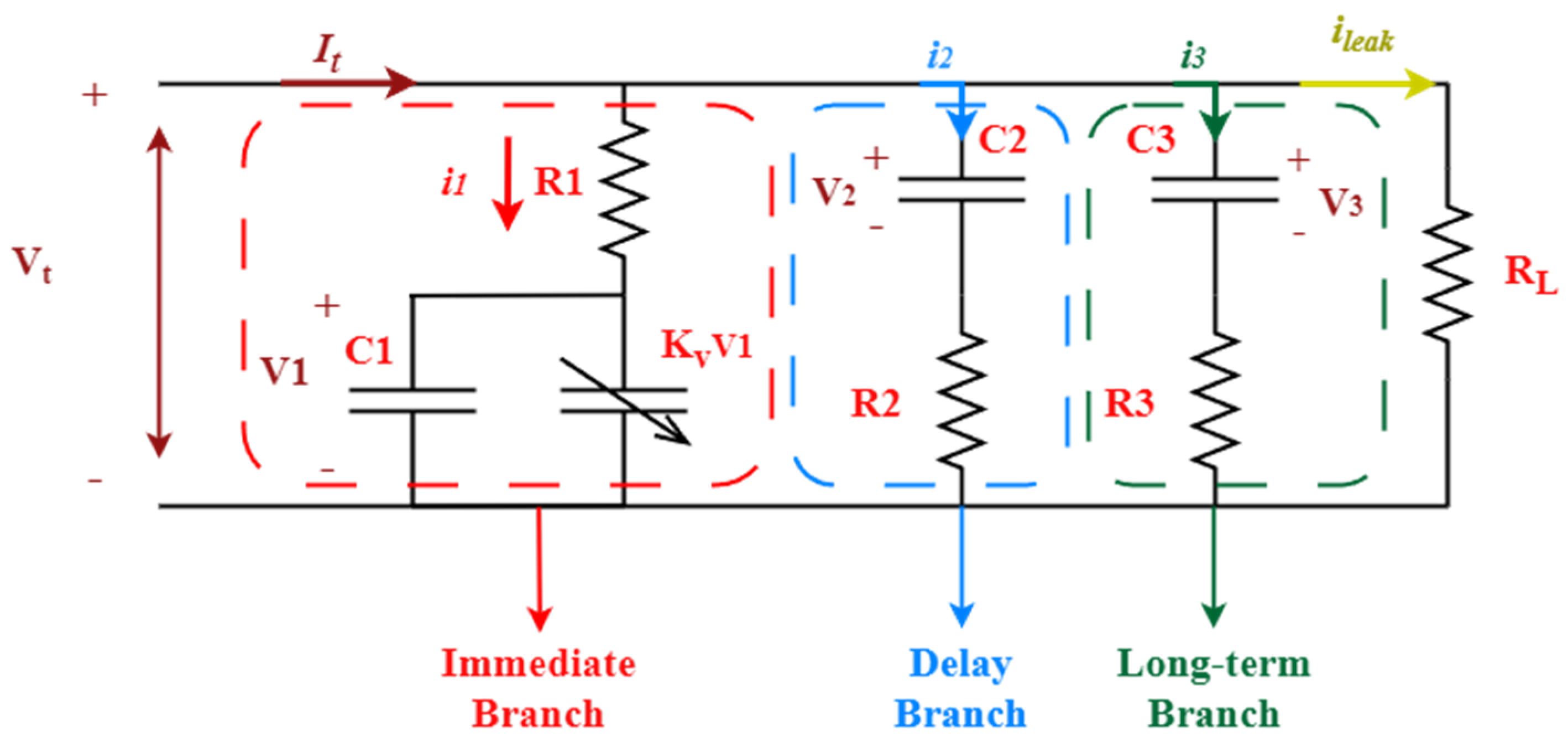
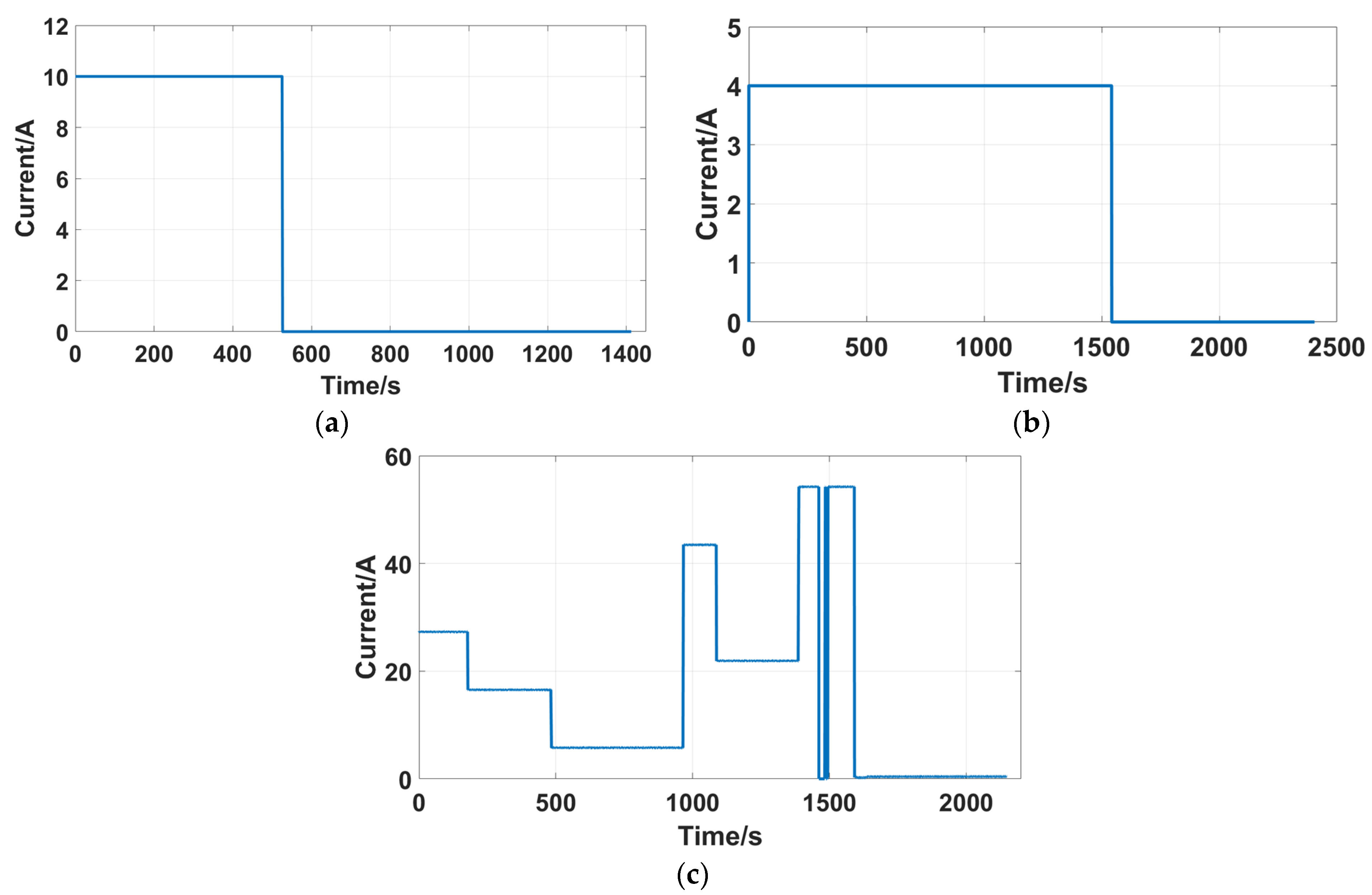
In this study, the Zubieta model parameters were determined for an SC bank comprising six capacitors in series, each with a rating of 2300 F, resulting in a total bank capacitance of 383.33 F. The estimation process involved using three different input signals: a step input with amplitudes of 10 A (Figure 4a) and 4 A (Figure 4b), along with a variable frequency input (Figure 4c), corresponding to profiles 1, 2, and 3 respectively. For each input, four distinct algorithms (M-MGBO, PSO, PSOLCEO, and PSO-MGBO) were executed in three separate runs. The Zubieta model, characterized by three branches, requires the estimation of a total of eight parameters, namely R 1 ,   R 2 ,   R 3 ,   C 1 ,   C 2 ,   C 3 ,   K v , and R L . Each of the algorithms (M-MGBO, PSO, PSOLCEO, and PSO-MGBO) requires initial guesses, which are formed using the analytical Zubieta model parameters and also using any initial guess selection rules the algorithms may have. These are detailed in the listings of each algorithm—for example, certain algorithms use the random initialization of the parameters’ values in the given bounds. The bounds themselves are derived using the parameters’ values derived using Zubieta’s analytical method. In each iteration of the respective algorithm, the parameters are estimated following the respective algorithmic procedures as outlined in Section 3. These estimated parameters are then used to estimate the supercapacitor terminal voltage at the given value of current, following Zubieta’s model equations. The mean square error between the measured and estimated supercapacitor terminal voltage, which is obtained using the estimated parameters, is used as the cost/fitness function to evaluate the fitness of the estimated parameters.
It is worth noting that the existence of a voltage-dependent capacitance in one of the Zubieta model’s branches makes this a nonlinear model. It is this nonlinear model that is used to evaluate the fitness of the estimated model parameters. Moreover, the MGBO algorithm used incorporates both gradient and population-based techniques to determine the search direction using Newton’s method. This search direction is based on a linear estimation of the gradient of the cost/fitness function. However, such approximation can make the algorithm prone to being stuck in a local optimum. To avoid this, the local escaping operator (LCEO)-based routine is used to augment the MGBO algorithm into the M-MGBO algorithm.

4.1. Parameters Estimation Results

The evaluation of the algorithms’ performance considered various criteria, including MSE and the computation time. Optimization took place on a personal computer equipped with an Intel(R) Xeon(R) E-2124 central processing unit operating at a frequency of 3.30 gigahertz and 16 gigabytes of random-access memory.
The cost function for the optimization problem was set to minimize the difference between the simulated SC voltage from the derived model and the actual measured voltage.
Minimize   SSE = t = 1 T   V t t V m t 2 ,
where V t ( t ) is the capacitor terminal voltage given by Equation (7) obtained using estimated model parameters, and V m (t) is the measured supercapacitor voltage.
The M-MGBO algorithm demonstrated superior performance compared with the other algorithms. In the case of Profile 1 (Table 3), M-MGBO and PSO-LCEO exhibited MSE values of 0.003927 and 0.003493, respectively. Notably, M-MGBO boasted the shortest computational time at 20,141.028 s, outperforming PSO-LCEO (26,782.93 s) and the hybrid PSO-MGBO (77,735.494 s). Additionally, parameters obtained by the M-MGBO algorithm were closer to analytically derived parameters (Table 2). For instance, the first branch capacitor C1 had a value of 0.7723 F with M-MGBO compared with 14.607195 F with PSO-LCEO.
The convergence curve plays a vital role in assessing optimization algorithms, offering insights into the speed and efficiency of their convergence to the optimal solution. Notably, the convergence curve for the M-MGBO algorithm stands out for its swift and stable convergence with minimal oscillation. While the PSO-LCEO algorithm also showed stable convergence, it did so at a slower pace compared with the M-MGBO algorithm. For Profile 1, Figure 9a illustrates the convergence curve of the best run for all four algorithms, showcasing the M-MGBO algorithm’s rapid convergence. Simultaneously, Figure 10a presents the voltage response for the same input.
Table 4 demonstrates the performance of the four optimization algorithms in estimating the parameters of a Zubieta supercapacitor model using Profile 2 as input. The M-MGBO algorithm exhibited the lowest MSE of 0.001001 and a significantly shortened computational time of 31,320.07 s. In contrast, the PSO-LCEO algorithm yielded a very similar MSE of 0.001017 compared with the M-MGBO algorithm. However, it exhibited a longer execution time of 36,297.98 s.
The hybrid PSO-MGBO and standard PSO algorithms exhibited higher MSE values of 0.01342 and 0.009034, respectively. In terms of average MSE, the M-MGBO algorithm outperformed others with a value of 0.001001, followed by the PSOL-CEO algorithm at 0.003169. The hybrid PSO-MGBO and regular PSO algorithms had higher average MSE values at 0.103347 and 0.107982, respectively. It is noteworthy that the LCEO operator, which is employed in the PSO-LCEO algorithm, serves as a method for escaping local optima during the optimization process. Despite this feature, the PSO-LCEO algorithm could not provide superior parameter estimates compared with the M-MGBO algorithm in this study. For the convergence curve of the best run for the four algorithms, refer to Figure 9b, while Figure 10b presents the corresponding voltage response.
The parameters obtained using Profile 3 input are presented in Table 5. The M-MGBO algorithm exhibited an MSE of 0.0042315, while the PSO-LCEO showed a comparable performance with an MSE of 0.004231. The hybrid PSO-MGBO had a similar MSE of 0.004231 but still outperformed the PSO-LCEO in terms of computational time, completing the task in only 32,206 s compared with 39,252 s. Notably, the M-MGBO algorithm showcased the best performance in terms of simulation time, with a runtime of 28,622 s.
It can be noted from the results that the M-MGBO and PSO-LCEO algorithms showed the best performance in terms of MSE, while the PSO-MGBO algorithm had a good balance between performance and simulation time. The PSO algorithm had the lowest computational time, but it had a significantly worse performance in terms of MSE. The convergence curve for the best run of the four algorithms is presented in Figure 9c, and the voltage response is presented in Figure 10c.

4.2. M-MGBO Results Validation

The results of 30 iterations of the M-MGBO method used to estimate the parameters of the Zubieta model of supercapacitors using a variable frequency input are presented in Table 6. The primary objective of this analysis is to assess the algorithm’s performance in terms of the consistency of parameter estimations, the accuracy of results pertaining to resistance and capacitance values, and any other noteworthy observations obtained from the table.
It is also important to consider the parameters’ standard deviation while analyzing the algorithm’s performance, as it provides a measure of the algorithm’s consistency. The standard deviation is a statistical measure used to assess the variability in parameter estimations across the 30 runs. Lower values of standard deviation indicate a higher level of consistency in the estimations. It is worth mentioning that certain parameters, including R 1   ( Ω ) and R 2   ( Ω ) , exhibit remarkably low standard deviation values, specifically 0.0009 and 0.02, respectively. The observed low values of standard deviation suggest that the M-MGBO algorithm exhibits a consistent pattern of convergence, yielding parameter estimations that are highly similar across every iteration. The level of consistency demonstrated in this context is of the utmost importance for practical applications, as it ensures the reliability and predictability of outcomes.

4.3. MGBO and M-MGBO Comparsion

To verify the reliability and assess the effectiveness of the modifications applied to the original MGBO algorithm, three separate runs were executed using the unaltered MGBO algorithm but with varying frequency inputs. The MGBO algorithm produced an average MSE of 0.0064, with a standard deviation of 5.7735 × 10⁻⁷ over the course of these three runs. Table 7 provides a comparative analysis between the M-MGBO and MGBO. Additionally, Figure 11 illustrates the convergence curve for the best-performing runs.
For K v the MGBO yielded a value of 53.0087 F/V, while the M-MGBO resulted in 51.7453 F/V. Despite the standard M-MGBO exhibiting a greater MSE when compared to the M-MGBO, it demonstrated a lower standard deviation for K v . Specifically, the standard deviation for K v was 0.0702 for the standard MGBO and 0.2311 for M-MGBO. This pattern is consistent for both R 3   and R L .

4.4. Parameters Testing

As demonstrated earlier, the M-MGBO method provides a more precise estimation of parameters concerning accuracy and MSE. To conduct additional testing on parameters from the four distinct methods, the optimal parameters acquired from the three runs (as presented in Table 4, Table 5 and Table 6) undergo further evaluation by interchanging and applying them to the remaining inputs. For example, parameters obtained using Profile 1 input are tested using Profile 2 and Profile 3 as inputs, and their mean squared error (MSE) is recorded.
Table 8 presents a scenario where parameters, initially estimated via Profile 1, were subsequently evaluated with Profile 2 and Profile 3 inputs. In the experiment with Profile 2, it is evident that the parameters of the M-MGBO algorithm yield the lowest MSE value of 1.4291. Furthermore, the PSO, PSO-MGBO, and PSO-LCEO had similar MSE values. Specifically, the PSO-LCEO algorithm demonstrated the second lowest MSE of 1.6312, followed by the PSO-MGBO method, with an MSE of 1.6396, and the PSO algorithm, with an MSE of 1.6442. When considering the use of parameters with Profile 3, it was seen that the M-MGBO algorithm exhibited the lowest MSE of 0.1195. Subsequently, the PSO-LCEO program showed an MSE of 0.1469, while the PSOGBO algorithm yielded an MSE of 0.1482. The PSO method demonstrated the most significant MSE value, measuring 0.4614.
Table 9 presents the results of the parameter testing conducted using parameters estimated using Profile 3 but tested with Profile 1 and Profile 2. The M-MGBO parameters yielded the lowest MSE in all tests. Specifically, the MSE was found to be 0.7448 for the Profile 2 input and 0.1754 for the Profile 1 input. The parameters of the PSO-LCEO algorithm exhibited the second-lowest MSE for both tests. Specifically, the MSE was found to be 0.7464 for the 4 A step input and 0.2001 for the 10 A step input.
The PSO-MGBO algorithm parameters have been determined to be the third-best performing algorithm, whereas the PSO algorithm exhibited the greatest mean MSE for both test cases. In a similar manner, while employing parameters estimated using Profile 2 tested with Profile 1 as input (Table 10), the same pattern emerged. The M-MGBO algorithm parameters yielded the lowest MSE value of 1.4149, followed by the PSO-LCEO and the PSO-MGBO, with MSE values of 1.5438 and 1.5349, respectively. In the instance of the Profile 3 input, the PSOL-CEO parameters yielded the lowest MSE of 0.9877, while the M-MGBO resulted in a slightly higher MSE of 0.9902. Furthermore, the particle swarm optimization (PSO) method yielded the highest MSE for both test scenarios.
To perform a more exhaustive evaluation of the algorithm’s parameters, two supplementary tests were conducted. These tests involved using a step input of 8 A (See Figure 12a) and a controlled current sequence as inputs. The optimal run parameters derived from prior experiments were used in both tests. Additionally, the performance is also assessed by comparing it to the analytical technique in order to validate the suitability of the parameters derived from the four algorithms.
As evident from Table 11, concerning the Profile 2 parameters, the M-MGBO algorithm demonstrates the lowest MSE at 0.9619, followed by the PSOLCEO with the second lowest MSE of 0.9793, and subsequently, the PSO-MGBO algorithm. In the case of the Profile 1 parameters, the PSO-LCEO showcased the lowest MSE of 0.1418, followed by the PSO-MGBO algorithm, while the M-MGBO ranked third, with an MSE of 0.2699. Profile 3 parameters exhibited a closely aligned response among M-MGBO, PSO-LCEO, and PSO-MGBO, displaying minimal deviation in MSE values. Conversely, the PSO algorithm, across various inputs, performed the least favorably, indicating higher MSE values and implying lower accuracy and reliability in the estimated parameter.
The controlled current sequence profile used for the following tests is illustrated in Figure 12b. According to the data presented in Table 12, it can be observed that the M-MGBO algorithm exhibited superior performance compared with the other algorithms and the analytical approach in terms of Profile 2 parameters. Specifically, the M-MGBO algorithm achieved an MSE value of 1.5037.
In the case of the Profile 1 parameters, it is evident that the M-MGBO algorithm exhibited superior performance compared with the other algorithms. The M-MGBO algorithm achieved an MSE of 0.0562, while the PSO-LCEO algorithm achieved an MSE of 0.2005, and the PSO-MGBO algorithm achieved an MSE of 0.5573. Nevertheless, the PSO-MGBO algorithm had the lowest performance in this particular test, as the PSO algorithm outperformed it, with an MSE value of 0.3547. Moreover, using Profile 3 parameters with the controlled current sequence profile, it was observed that the M-MGBO algorithm demonstrated superior performance in comparison to the other algorithms, achieving an MSE of 0.0483. On the other hand, the PSO, PSO-LCEO, and PSO-MGBO algorithms demonstrated a similar performance, with minimal deviation in MSE values.

5. Conclusions

The importance of energy storage for grid stability and power backup in both conventional and renewable systems is evident. Particularly, supercapacitors stand out for their excellence in high-power density applications, such as regenerative braking in electric vehicles. This research concentrates on the parameterization of the Zubieta model tailored for supercapacitors, employing a hybrid metaheuristic gradient-based optimization (MGBO) strategy. The Zubieta model, featuring three RC branches and a self-discharge branch, necessitates the identification of seven parameters. The investigation systematically compared the performance of the modified MGBO (M-MGBO) against particle swarm optimization (PSO) and two variations—one integrating PSO with M-MGBO and the other introducing a local escaping operator (LCEO). The evaluation encompasses key metrics like convergence rate, accuracy, and processing/computational time. The results indicate that both hybrid PSO-MGBO and PSO-LCEO surpass conventional PSO, exhibiting enhancements of 51% and 94%, respectively. Remarkably, these variants proved to be comparable to M-MGBO. These methodologies effectively contribute to the accurate estimation of Zubieta model parameters, The study underscores the considerable potential of hybrid optimization strategies in advancing the precision and effectiveness of supercapacitor model parameterization.
The findings showed M-MGBO’s adaptability to diverse operational contexts, with specific examples of a computational time of 31,320.07 s under a 4 A step input. Delving into the consistency and reliability of M-MGBO, the study scrutinized standard deviation values across 30 runs, revealing a remarkably stable pattern. This consistency is pivotal for practical applications, ensuring predictability and reliability in outcomes. The meticulous examination of the algorithm’s performance underscored its reliability, with a computational time of approximately 28,610 s across 30 runs, adhering to the expected order of magnitude in resistance and capacitance values with respect to the analytical approach. As reported in the literature, when using metaheuristic algorithms the search for the optimal solution can become caught in local optima in most nonlinear systems with more than one minimum. Moreover, they do not always guarantee the global optimum solution and only provide nearly optimal solutions. This paper attempts to overcome these challenges by proposing some novel updates to the metaheuristic algorithms, and further improvements are left for future efforts.

Author Contributions

Conceptualization, A.Y., R.D. and S.M.; methodology, A.Y., R.D. and S.M.; software, A.Y.; validation, A.Y.; formal analysis, A.Y., R.D. and S.M.; investigation, A.Y., R.D. and S.M.; resources, A.Y., R.D. and S.M.; data curation, A.Y; writing—original draft preparation, A.Y.; writing—review and editing, A.Y., R.D. and S.M.; visualization, A.Y.; supervision, R.D. and S.M. All authors have read and agreed to the published version of the manuscript.

Funding

The work in this paper was supported, in part, by the Open Access Program from the American University of Sharjah.

Data Availability Statement

All data required can be generated using the equations/algorithms presented in this work. Experimental data requires experimentation with the appropriate hardware apparatus as shown in the paper.

Acknowledgments

This paper represents the opinions of the authors and does not mean to represent the position or opinions of the American University of Sharjah.

Conflicts of Interest

Authors declare no conflicts of interest.

References

  1. Sayed, E.T.; Olabi, A.G.; Alami, A.H.; Radwan, A.; Mdallal, A.; Rezk, A.; Abdelkareem, M.A. Renewable Energy and Energy Storage Systems. Energies 2023, 16, 1415. [Google Scholar] [CrossRef]
  2. Olabi, A.; Onumaegbu, C.; Wilberforce, T.; Ramadan, M.; Abdelkareem, M.A.; Alami, A.H.A. Critical review of energy storage systems. Energy 2021, 214, 118987. [Google Scholar] [CrossRef]
  3. Salameh, T.; Abdelkareem, M.A.; Olabi, A.G.; Sayed, E.T.; Al-Chaderchi, M.; Rezk, H. Integrated standalone hybrid solar PV, fuel cell and diesel generator power system for battery or supercapacitor storage systems in Khorfakkan, United Arab Emirates. Int. J. Hydrogen Energy 2021, 46, 6014–6027. [Google Scholar] [CrossRef]
  4. Rezk, H.; Nassef, A.M.; Abdelkareem, M.A.; Alami, A.H.; Fathy, A. Comparison among various energy management strategies for reducing hydrogen consumption in a hybrid fuel cell/supercapacitor/battery system. Int. J. Hydrogen Energy 2021, 46, 6110–6126. [Google Scholar] [CrossRef]
  5. Adib, A.; Dhaouadi, R. Modeling and analysis of a regenerative braking system with a battery-supercapacitor energy storage. In Proceedings of the 2017 7th International Conference on Modeling, Simulation, and Applied Optimization (ICMSAO), Sharjah, United Arab Emirates, 4–6 April 2017. [Google Scholar] [CrossRef]
  6. Zhang, J.; Gu, M.; Chen, X. Supercapacitors for renewable energy applications: A review. Micro Nano Eng. 2023, 21, 100229. [Google Scholar] [CrossRef]
  7. Naseri, F.; Karimi, S.; Farjah, E.; Schaltz, E. Supercapacitor management system: A comprehensive review of modeling, estimation, balancing, and protection techniques. Renew. Sustain. Energy Rev. 2022, 155, 111913. [Google Scholar] [CrossRef]
  8. Haris, M.; Hasan, M.N.; Qin, S. State of health prediction of supercapacitors using multi-trend learning of NARX neural network. Mater. Today Sustain. 2022, 20, 100201. [Google Scholar] [CrossRef]
  9. Liu, C.; Li, Q.; Wang, K. State-of-charge estimation and remaining useful life prediction of supercapacitors. Renew. Sustain. Energy Rev. 2021, 150, 111408. [Google Scholar] [CrossRef]
  10. Mehta, U.; Prasad, R.; Kothari, K. Various analytical models for supercapacitors: A mathematical study. Resour. Technol. 2020, 1, 1–15. [Google Scholar] [CrossRef]
  11. Mukhopadhyay, S.; Dhaouadi, R.; Takrouri, M.; Dogga, R. Supercapacitor Characterization Using Universal Adaptive Stabilization and Optimization. IEEE Open J. Ind. Electron. Soc. 2020, 1, 166–183. [Google Scholar] [CrossRef]
  12. Chen, Y.; Yan, R.; Yu, C.; Zhao, C.; Huang, X.; Wei, L. Investigation on Characteristic Parameters Identification and Evolution of Supercapacitor Energy Storage System From Sparse and Fragmented Monitoring Data. IEEE Access 2023, 11, 56983–56993. [Google Scholar] [CrossRef]
  13. Zhang, L.; Hu, X.; Wang, Z.; Sun, F.; Dorrell, D.G. A review of supercapacitor modeling, estimation, and applications: A control/management perspective. Renew. Sustain. Energy Rev. 2018, 81, 1868–1878. [Google Scholar] [CrossRef]
  14. Hetzel, M.; Ocampo, D.D.; De Carne, G.; Hiller, M. Supercapacitor Modeling and Parameter Identification of a 400 kW Grid-Connected Supercapacitor Energy Storage System using the Inherent Impedance Spectroscopy Capability of its DC/DC Converter. In Proceedings of the 2023 IEEE Energy Conversion Congress and Exposition (ECCE), Nashville, TN, USA, 29 October 29–2 November 2023; pp. 459–465. [Google Scholar]
  15. Majchrzycki, W.; Jankowska, E.; Baraniak, M.; Handzlik, P.; Samborski, R. Electrochemical Impedance Spectroscopy and Determination of the Internal Resistance as a Way to Estimate Lead-Acid Batteries Condition. Batteries 2018, 4, 70. [Google Scholar] [CrossRef]
  16. Barcellona, S.; Ciccarelli, F.; Iannuzzi, D.; Piegari, L. Modeling and parameter identification of lithium-ion capacitor modules. IEEE Trans. Sustain. Energy 2014, 5, 785–794. [Google Scholar] [CrossRef]
  17. Chatterjee, K.; Agnihotri, P.K.; Basu, S.; Gupta, N. Quantification of Pore Accessibility in Mesoporous Supercapacitor Electrode Using Cyclic Voltammetry. IEEE Trans. Instrum. Meas. 2023, 73, 3341125. [Google Scholar] [CrossRef]
  18. Zucca, M.; Hassanzadeh, M.; Conti, O.; Pogliano, U. Accurate Parameters Identification of a Supercapacitor Three-Branch Model. IEEE Access 2023, 11, 122387–122398. [Google Scholar] [CrossRef]
  19. Marín-Coca, S.; Ostadrahimi, A.; Bifaretti, S.; Roibás-Millán, E.; Pindado, S. New Parameter Identification Method for Supercapacitor Model. IEEE Access 2023, 11, 21771–21782. [Google Scholar] [CrossRef]
  20. Zubieta, L.; Bonert, R. Characterization of double-layer capacitors for power electronics applications. IEEE Trans. Ind. Appl. 2000, 36, 199–205. [Google Scholar] [CrossRef]
  21. Krishnan, G.; Das, S.; Agarwal, V. An Online Identification Algorithm to Determine the Parameters of the Fractional-Order Model of a Supercapacitor. IEEE Trans. Ind. Appl. 2020, 56, 763–770. [Google Scholar] [CrossRef]
  22. Wang, J.; Zhang, L.; Mao, J.; Zhou, J.; Xu, D. Fractional Order Equivalent Circuit Model and SOC Estimation of Supercapacitors for Use in HESS. IEEE Access 2019, 7, 52565–52572. [Google Scholar] [CrossRef]
  23. Reichbach, N.; Kuperman, A. Recursive-Least-Squares-Based Real-Time Estimation of Supercapacitor Parameters. IEEE Trans. Energy Convers. 2016, 31, 810–812. [Google Scholar] [CrossRef]
  24. Xu, D.; Zhang, L.; Wang, B.; Ma, G. A novel equivalent-circuit model and parameter identification method for supercapacitor performance. Energy Procedia 2018, 145, 133–138. [Google Scholar] [CrossRef]
  25. Xu, D.; Zhang, L.; Wang, B.; Ma, G. Modeling of Supercapacitor Behavior with an Improved Two-Branch Equivalent Circuit. IEEE Access 2019, 7, 26379–26390. [Google Scholar] [CrossRef]
  26. Wei, T.; Qi, X.; Qi, Z. An improved ultracapacitor equivalent circuit model for the design of energy storage power systems. In Proceedings of the 2007 International Conference on Electrical Machines and Systems, Seoul, Republic of Korea, 8–11 October 2007; pp. 69–73. [Google Scholar] [CrossRef]
  27. Pucci, M.; Vitale, G.; Cirrincione, G.; Cirrincione, M. Parameter identification of a Double-Layer-Capacitor 2-branch model by a least-squares method. In Proceedings of the IECON 2013—39th Annual Conference of the IEEE Industrial Electronics Society, Vienna, Austria, 10–13 November 2013; pp. 6770–6776. [Google Scholar] [CrossRef]
  28. Faranda, R. A new parameters identification procedure for simplified double layer capacitor two-branch model. Electr. Power Syst. Res. 2010, 80, 363–371. [Google Scholar] [CrossRef]
  29. Zhang, L.; Wang, Z.; Sun, F.; Dorrell, D.G. Online Parameter Identification of Ultracapacitor Models Using the Extended Kalman Filter. Energies 2014, 7, 3204–3217. [Google Scholar] [CrossRef]
  30. Kennedy, J.; Eberhart, R. Particle Swarm Optimization. In Proceedings of the ICNN’95—International Conference on Neural Networks, Perth, Australia, 27 November–1 December 1995; Volume 4, pp. 1942–1948. [Google Scholar] [CrossRef]
  31. Mirjalili, S.; Mirjalili, S.M.; Lewis, A. Grey Wolf Optimizer. Adv. Eng. Softw. 2014, 69, 46–61. [Google Scholar] [CrossRef]
  32. Mirjalili, S.; Lewis, A. The Whale Optimization Algorithm. Adv. Eng. Softw. 2016, 95, 51–67. [Google Scholar] [CrossRef]
  33. Mirjalili, S. The Ant Lion Optimizer. Adv. Eng. Softw. 2015, 83, 80–98. [Google Scholar] [CrossRef]
  34. Holland, J.H. Adaptation in Natural and Artificial Systems: An Introductory Analysis with Applications to Biology, Control, and Artificial Intelligence; MIT Press: Cambridge, CA, USA, 1992. [Google Scholar]
  35. Zhao, W.; Wang, L.; Zhang, Z. Artificial ecosystem-based optimization: A novel nature-inspired meta-heuristic algorithm. Neural Comput. Appl. 2020, 32, 9383–9425. [Google Scholar] [CrossRef]
  36. Nassef, A.M.; Fathy, A.; Rezk, H.; Yousri, D. Optimal parameter identification of supercapacitor model using bald eagle search optimization algorithm. J. Energy Storage 2022, 50, 104603. [Google Scholar] [CrossRef]
  37. Fathy, A.; Rezk, H. Robust electrical parameter extraction methodology based on Interior Search Optimization Algorithm applied to supercapacitor. ISA Trans. 2020, 105, 86–97. [Google Scholar] [CrossRef]
  38. Gandomi, A.H. Interior search algorithm (ISA): A novel approach for global optimization. ISA Trans. 2014, 53, 1168–1183. [Google Scholar] [CrossRef]
  39. Sun, G.; Liu, Y.; Chai, R.; Mei, F.; Zhang, Y. Online model parameter identification for supercapacitor based on weighting bat algorithm. AEU—Int. J. Electron. Commun. 2018, 87, 113–118. [Google Scholar] [CrossRef]
  40. Mostafaoui, M.; Benyoucef, D. Electrical model parameters identification of radiofrequency discharge in argon through 1D3V/PIC-MC model. Plasma Sci. Technol. 2018, 20, 095401. [Google Scholar] [CrossRef]
  41. Zhao, Y.; Xie, W.; Fang, Z.; Liu, S. A Parameters Identification Method of the Equivalent Circuit Model of the Supercapacitor Cell Module Based on Segmentation Optimization. IEEE Access 2020, 8, 92895–92906. [Google Scholar] [CrossRef]
  42. Goh, C.-T.; Cruden, A. Bivariate quadratic method in quantifying the differential capacitance and energy capacity of supercapacitors under high current operation. J. Power Sources 2014, 265, 291–298. [Google Scholar] [CrossRef]
  43. Zhao, Y.; Wei, L. Structure and Parameter Identification of Supercapacitors Based on Particle Swarm Optimization. Zhongguo Dianji Gongcheng Xuebao 2012, 32, 155–161. [Google Scholar]
  44. Raouti, D.; Flazi, S.; Benyoucef, D. Modeling and Identification of Electrical Parameters of Positive DC Point-to-Plane Corona Discharge in Dry Air Using RLS Method. IEEE Trans. Plasma Sci. 2016, 44, 1144–1149. [Google Scholar] [CrossRef]
  45. Mirjalili, S. SCA: A Sine Cosine Algorithm for solving optimization problems. Knowl.-Based Syst. 2016, 96, 120–133. [Google Scholar] [CrossRef]
  46. Abbassi, R.; Saidi, S.; Abbassi, A.; Jerbi, H.; Kchaou, M.; Alhasnawi, B.N. Accurate Key Parameters Estimation of PEMFCs’ Models Based on Dandelion Optimization Algorithm. Mathematics 2023, 11, 1298. [Google Scholar] [CrossRef]
  47. Abbassi, R.; Saidi, S.; Urooj, S.; Alhasnawi, B.N.; Alawad, M.A.; Premkumar, M. An Accurate Metaheuristic Mountain Gazelle Optimizer for Parameter Estimation of Single- and Double-Diode Photovoltaic Cell Models. Mathematics 2023, 11, 4565. [Google Scholar] [CrossRef]
  48. Ahmadianfar, I.; Bozorg-Haddad, O.; Chu, X. Gradient-based optimizer: A new metaheuristic optimization algorithm. Inf. Sci. 2020, 540, 131–159. [Google Scholar] [CrossRef]
  49. Ahmadianfar, I.; Gong, W.; Heidari, A.A.; Golilarz, N.A.; Samadi-Koucheksaraee, A.; Chen, H. Gradient-based optimization with ranking mechanisms for parameter identification of photovoltaic systems. Energy Rep. 2021, 7, 3979–3997. [Google Scholar] [CrossRef]
  50. Shami, T.M.; El-Saleh, A.A.; Alswaitti, M.; Al-Tashi, Q.; Summakieh, M.A.; Mirjalili, S. Particle Swarm Optimization: A Comprehensive Survey. IEEE Access 2022, 10, 10031–10061. [Google Scholar] [CrossRef]
  51. Clerc, M.; Kennedy, J. The particle swarm—Explosion, stability, and convergence in a multidimensional complex space. IEEE Trans. Evol. Comput. 2002, 6, 58–73. [Google Scholar] [CrossRef]
  52. Hafez, I.; Dhaouadi, R. Identification of Mechanical Parameters in Flexible Drive Systems Using Hybrid Particle Swarm Optimization Based on the Quasi-Newton Method. Algorithms 2023, 16, 371. [Google Scholar] [CrossRef]
  53. Usman, H.M.; Mukhopadhyay, S.; Rehman, H. Universal Adaptive Stabilizer Based Optimization for Li-Ion Battery Model Parameters Estimation: An Experimental Study. IEEE Access 2018, 6, 49546–49562. [Google Scholar] [CrossRef]
Figure 1. Supercapacitor Zubieta model.
Energies 17 01500 g001
Figure 2. Supercapacitor Zubieta model Simulink representation: (a) long-term branch; (b) delayed branch; (c) main model; (d) immediate branch.
Energies 17 01500 g002aEnergies 17 01500 g002b
Figure 3. Experimental setup block diagram.
Energies 17 01500 g003
Figure 4. Experimental current profiles: (a) Profile 1: 10 A step input; (b) Profile 2: 4 A step input; (c) Profile 3: Variable frequency input.
Energies 17 01500 g004
Figure 5. Experimental voltage response vs. the analytical response using current Profile 1.
Energies 17 01500 g005
Figure 6. PSO flow chart.
Energies 17 01500 g006
Figure 7. Comparison between α and C .
Energies 17 01500 g007
Figure 8. Flow chart hybrid PSO-MGBO method developed in this work. P b e s t is the personal best solution, and G B e s t is the global best solution. Text in red indicates the related steps to the M-MGBO algorithm.
Energies 17 01500 g008
Figure 9. (a) Convergence curve for Profile 1, (b) Convergence curve for Profile 2, and (c) Convergence curve for Profile 3.
Energies 17 01500 g009
Figure 10. (a) Voltage response for Profile 1, (b) Voltage response for Profile 2, and (c) Voltage response for Profile 3.
Energies 17 01500 g010
Figure 11. Best run convergence curve comparison between M-GBO and M-MGBO for variable frequency input.
Energies 17 01500 g011
Figure 12. (a) 8 A step input, (b) Controlled current sequence.
Energies 17 01500 g012
Table 1. Zubieta model analytical parameterization procedure.
ParameterRelationComments
R 1 R 1 = V 1 i s c The SC is assumed to start charging at zero initial conditions. V1 is the voltage at t1 where 20 ms < t1 < 50 ms
C 1 C 1 = i s c t 2 t 1 V Where t2 is the time when V = V 2 V 1 = 50   m V
K v K v = 2 V 4 ( Q t V 4 C o ) Where the amount of charge stored Qt = isc(t4 − t1), and t4 = t3 + 20 ms. Where t3 is when Vsc = Vrated
R 2 R d = V 4 V 2 2 t 5 t 4 ( C o + k V 4 V 2 2 ) V 2 Where t5 is at V5 = V4 V 2 . Where V 2 = 50   m V
C 2 C 2 = Q t V 6 ( C o + k V 6 2 ) V6 is the voltage at t6 = t5 + 300 s
R 3 R 3 = V 7 V 2 2 t 7 t 6 ( C o + k V 6 V 2 2 ) V 2 Where t7 is at V7 = V6 V 2 . Where V 2 = 50   m V
C 3 C 3 = Q t V 7 ( C o + k V 7 2 ) C _ 2   Where V8 is at t8 = 30 min
Table 2. Identified SC parameters using Zubieta model analytical parameterization procedure.
ParameterValue
K v ( F V ) 53.4472
R 1 ( Ω ) 0.0041
C 1 ( F ) 0.8516
R 2 ( Ω ) 0.0024
C 2 ( F ) 69.7146
R 3 ( Ω ) 4.9780
C 3 ( F ) 126.8252
T 1 0.00349156
T 2 0.167315
T 3 631.4593
Table 3. Experimental results for the parameters estimated using current Profile 1 with 150 iterations (T1, T2, and T3 are the respective branches’ time constants).
ParameterM-MGBOPSOPSO-LCEOPSO-MGBO
K v ( F V ) 38.4592998414.0739833.2239833.266903
R 1 ( Ω ) 0.0131630460.1270280.0140340.04586
C 1 ( F ) 0.7723287748.1306214.607190.95056
R 2 ( Ω ) 0.4877895465.1900330.43961.61732
C 2 ( F ) 224.0938314 154.1119168.6782175.7074
R 3 ( Ω ) 36.73460650421.079124.80773942.54308
C 3 ( F ) 394.158958331.8499214.2253243.417
R l ( Ω ) 25.7046283368.1327362.4767637.94408
MSE0.0039273910.0573140.0034940.025034
Elapsed Time20141.02816564.04026782.93077735.494
T10.0101666.1139360.2049970.043593
T2109.3106799.845874.15094284.1751
T314479.276995.1041029.93910355.71
Average MSE0.0068130.075816930.0087894730.03842393
Table 4. Experimental results for the parameters estimated using current Profile 2 with 150 iterations (T1, T2, and T3 are the respective branches’ time constants).
ParameterM-MGBOPSOPSO-LCEOPSO-MGBO
K v ( F V ) 37.280585927.813136.435936.86813
R 1 ( Ω ) 0.058352970.075560.0561840.149894
C 1 ( F ) 0.0330758817.9570.6272310.105358
R 2 ( Ω ) 0.695755190.59430.7017025.188335
C 2 ( F ) 228.197898163.674226.8816198.3325
R 3 ( Ω ) 24.470379331.625518.6283337.35831
C 3 ( F ) 394.767419330.281273.4351251.036
R l ( Ω ) 52.35864856.049394.785463.34033
MSE0.00100130.013420.0010170.009034
Elapsed Time31320.0710926036297.9822324.22
T10.001931.3568310.035240.015793
T2158.769997.27146159.20331029.015
T39660.10810445.35093.6399378.281
Average MSE0.0010010.1033470.00316930.107982
Table 5. Experimental results for the parameters estimated using a variable frequency current profile with 150 iterations (T1, T2, and T3 are the respective branches’ time constants).
ParameterM-MGBOPSOPSO-LCEOPSO-MGBO
K v ( F V ) 51.74533692125.41551.7280951.74644
R 1 ( Ω ) 0.0802658420.13460.0804510.015515
C 1 ( F ) 0.01278360971.440.0021660.572341
R 2 ( Ω ) 0.5726827018.903770.5717990.080359
C 2 ( F ) 223.6858074186.193223.5703223.6356
R 3 ( Ω ) 49.9994771324.5265049.99997
C 3 ( F ) 399.9692153292.147400400
R l ( Ω ) 20.9065818931.460420.8664220.90162
MSE0.0042315440.300360.0042310.004231
Elapsed Time28622.5119519408.0052739252.5936232206.02127
T10.0010269.6158240.0001740.00888
T2128.1011657.82127.837317.97113
T319998.257165.1972000019999.99
Average MSE0.0042335050.2269217810.0109020.004257128
Table 6. Experimental results for the parameters using M-MGBO and variable frequency with 30 runs (T1, T2, and T3 are the respective branches’ time constants).
ParameterStandard DeviationAverage
K v ( F V ) 0.34604951.95607
R 1 ( Ω ) 0.0009670.079637
C 1 ( F ) 0.0050860.01552
R 2 ( Ω ) 0.021330.555367
C 2 ( F ) 0.129872223.7431
R 3 ( Ω ) 0.07090849.96596
C 3 ( F ) 0.912619399.2558
R l ( Ω ) 0.40576721.18428
T10.0003930.001233
T24.766871124.2593
T372.7569519949.26
Table 7. Comparison of M-MGBO and M-MGBO best run 150 iterations (T1, T2, and T3 are the respective branches’ time constants).
ParameterMGBOM-MGBO
K v ( F V ) 53.0086751.74533692
R 1 ( Ω ) 0.2293190.080265842
C 1 ( F ) 0.04882780.012783609
R 2 ( Ω ) 0.8723460.572682701
C 2 ( F ) 223.6373223.6858074
R 3 ( Ω ) 5049.99947713
C 3 ( F ) 399.9993399.9692153
R l ( Ω ) 20.9098820.90658189
T1127.997817.9543
T219999.9719998.2516
T353.0086751.74533692
MSE0.00635710.004231544
Table 8. MSE for Profile 1 parameters tested with Profiles 2 and 3 as inputs.
AlgorithmProfile 2 (4A Input)Profile 3 (Variable Frequency Input)
MGBO----0.1489
PSO-GBO1.63960.1482
M-MGBO1.42910.1195
PSO-LCEO1.63120.1469
PSO1.64420.4614
Table 9. MSE for Profile 3 parameters tested with Profiles 1 and 2 as inputs.
AlgorithmProfile 2 (4 A Input)Profile 1 (10 A Input)
MGBO--------
PSO-MGBO0.81440.5252
M-MGBO0.74480.1754
PSOL-CEO0.74640.2001
PSO0.86450.5794
Table 10. M-MGBO variable frequency 30 runs parameters standard deviation and average.
AlgorithmProfile 1 (10 A Input)Profile 3 (Variable Frequency Input)
MGBO----1.2619
PSO-MGBO1.53490.9896
M-MGBO1.41490.9902
PSO-LCEO1.54380.9877
PSO1.69301.2362
Table 11. Terminal voltage MSE for test using 8A profile, with parameters estimated using profiles 1, 2, and 3 and the analytical approach parameters.
AlgorithmProfile 2 (4 A Parameters)Profile 1 (10 A Parameters)Profile 3 (Variable Frequency Parameters)
PSO-MGBO0.98480.16170.0942
M-MGBO0.96190.26990.0943
PSO-LCEO0.97930.14180.0945
PSO1.13250.28240.3063
Analytical7.7745
Table 12. Terminal voltage MSE for test using controlled current sequence profile, with parameters estimated using profiles 1, 2, and 3 and the analytical approach parameters.
AlgorithmProfile 2 (4 A Parameters)Profile 1 (10 A Parameters)Profile 3 (Variable Frequency Parameters)
PSO-MGBO2.16810.55730.0571
M-MGBO1.50370.05620.0483
PSO-LCEO1.57780.20050.05765
PSO2.12510.35470.0570
Analytical7.364942
Disclaimer/Publisher’s Note: The statements, opinions and data contained in all publications are solely those of the individual author(s) and contributor(s) and not of MDPI and/or the editor(s). MDPI and/or the editor(s) disclaim responsibility for any injury to people or property resulting from any ideas, methods, instructions or products referred to in the content.

