Article

Useful Exergy as an Intermediate Input in a Two-Sector Model of the United States Economy

1
MARETEC—Marine, Environment and Technology Center, Instituto Superior Técnico (IST), University of Lisbon, Avenida Rovisco Pais 1, 1049-001 Lisbon, Portugal
2
Engineering Department, Calvin University, 3201 Burton St. SE, Grand Rapids, MI 49546, USA
3
Sustainability Research Institute, School of Earth and Environment, University of Leeds, Leeds LS2 9JT, UK
4
School for Public Leadership, Faculty of Economic and Management Science, Stellenbosch University, Matieland 7602, South Africa
*
Author to whom correspondence should be addressed.
Energies 2024, 17(6), 1481; https://doi.org/10.3390/en17061481
Submission received: 7 February 2024 / Revised: 4 March 2024 / Accepted: 12 March 2024 / Published: 20 March 2024
(This article belongs to the Section C: Energy Economics and Policy)

Abstract

:
Conventional economic growth models treat production/consumption as abstractions linked only by money flows, disregarding their connection to the physical world. Nevertheless, the existing literature suggests that energy flows can influence production and links useful exergy prices with economic growth. Useful exergy is energy measured at the stage where it produces an end-use (and is a measurement of energy quality). Not all approaches in the literature use this metric and they often consider energy as a primary input (despite it being an intermediate input). We explore the relationship between energy flows and economic growth for the US through a framework where useful exergy, the output of an “extended energy sector” (where all effects of increasing primary-to-final-to-useful exergy efficiency are located), is an intermediate input for a “non-energy sector”. Together, they encompass the entire economy. We conclude that the share of investment in the extended energy sector grew with the overall economic growth throughout 1960–2020, while the labour share decreased. The non-energy sector contributed the largest share of consumption, exports, imports and labour. In recent years, the energy sector has overtaken it in terms of investment. Our two-sector model has important implications for current climate policy, namely regarding the Integrated Assessment Models on which it is based.

1. Introduction

In neoclassical economic theory, the primary inputs to production are capital and labour. With the advent of GDP and other economic time series, empirical data showed that capital played a much smaller role in past economic growth than had previously been assumed [1]. In neoclassical economic growth theory, as articulated by Solow-Swan and others, an aggregate production function of capital stock and labour supply was introduced, but it left most of the historical growth up to that point unexplained [2], leading to the creation of the term “total factor productivity” to describe this residual growth. This total factor productivity is yet to be fully understood, but ecological economists argue it could be due to the failure of economic models to account for the interaction between the economy and the physical world, namely material and energy flows [3,4].
Neoclassical growth theory considers capital stock and labour as the “primary factors of production” (meaning they contribute to the production process but are neither significantly altered by it nor part of its final product), sometimes with a “technology factor”. Energy is thus classified as an intermediate input which can be “produced” by a combination of primary factors of production [5]. The cost-share theorem, which is widely accepted among mainstream economists, tells us that factors of production are needed in proportion to their productivities and that the output productivity of each factor is equal to its cost-share (about 30% for capital and 70% for labour in the US from 1960 up to now, with small deviations [6]), which has led to energy being disregarded as a factor of production due to its historically low cost-share (less than 10%, if it is even considered) [7,8].
Ecological economic models do not presuppose an equivalency between cost-share and productivity, opting instead to estimate productivity statistically, which leads to much higher estimated levels of productivity for energy than expected from its cost-share. These models have also attempted to emphasize the role of energy in economic growth by treating it as an independent primary factor of production alongside capital and labour [9]. The most innovative of these approaches argue that long-term growth is not driven by total energy consumption, but by useful exergy, which is the flow of energy that actually ends up producing economic value [10,11,12,13]. Recent research also argues that a major driver of economic growth is the technological improvement in primary-to-final-to-useful exergy efficiency, which is reflected in decreasing useful exergy prices [9,10,14].
These ecological economic models have not been accepted by the mainstream economics community for violating the cost-share theorem, according to which energy should have a much lower productivity. We argue that the role that energy plays in economic growth has been underestimated [15,16,17] by neoclassical economics. Nevertheless, we also find the usual approach used in the ecological economics literature, of treating energy as a primary input, to be inconsistent. Instead, we choose to treat it correctly as an intermediate input and to measure it with the useful exergy metric. We do this by using a two-sector model of the economy, which we adapted for the case of the US, where we separate the primary-to-final-to-useful exergy transformation processes from the remaining productive activities. This also allows us to isolate the effects of technological progress in exergy transformation efficiency in a single sector.
Our methodology is adapted from the work on the Portuguese economy in Santos et al. [18]. We chose to focus on the US as it has been the world’s largest economy by nominal GDP for almost the entirety of the time period studied, as well as being an advanced economy characterised by a diverse array of industries and sectors.
In addition to the debate on whether or not energy flows should be taken into account when discussing economic growth, there is a debate on the most relevant metric to use for energy. In this work, we chose to measure energy with the exergy metric, its most physically significant form for economic studies [19,20].
Regarding energy transformation, the primary energy stage is the stage in which energy exists in nature prior to any transformation or human interference (e.g., a lump of coal underground). The final energy stage is the stage in which energy is sold to firms or households (e.g., the electricity we receive from the grid). The useful energy stage is the stage in which energy is delivered to an economically productive end-use, before being converted into energy services. Nevertheless, not all forms of useful energy are qualitatively equivalent.
According to the Second Law of Thermodynamics, in irreversible physical transformations of energy, only some of it (exergy) can be used to perform useful work, while the rest (anergy) is lost. For instance, 1 kWh of work can be converted into up to 1 kWh of heat at 30 °C, but 1 kWh of heat at 30 °C can be converted into a maximum of 0.066 kWh of work (assuming that the environment is at a temperature of 10 °C). Accounting for energy with the exergy metric, then, changes the way heat and work are added up, acknowledging that energy forms are different and allowing us to quantify their quality. For instance, 1 kWh of work is much more valuable than 1 kWh of heat. Exergy, the potential of an energy flow to perform physical work until it achieves equilibrium with the environment, thus measures thermodynamic energy quality.
This means that, while energy is usually accounted for in economics at the final energy stage, which is the last stage at which it is priced, only the useful exergy share of this final energy will actually produce economic value. Furthermore, this means that measuring energy at the useful exergy stage takes into account the technological improvement in primary-to-final-to-useful exergy efficiency, allowing us to directly assess the impact of this improvement on economic growth. This is consistent with the argument that long-term economic growth is linked to useful exergy use, with the declining prices of useful exergy having been cited as the major engine of economic growth [11].
Our goal in this work is to study the relationship between economic production and exergy flows and to analyse how economic development is impacted by exergy usage. In Section 2, we go through the method employed in this work (adapted from Santos et al. [18]), namely how the disaggregation and reclassification of national accounts data on consumption, investment, exports and imports, capital, labour, gross operating surplus, compensation of employees and taxes minus subsidies on production and imports was carried out. We carry out the same for exergy flows, considering the energy carrier, institutional sector where energy is consumed and category of end-use. We also present the datasets used for the disaggregation and reclassification of each macroeconomics variable studied, as well as exergy. In Section 3, we show the results of the reclassification of each of these variables under the two-sector model framework and discuss them quantitatively. Finally, in Section 4, we draw some conclusions about what our results tell us about the economic development of the US in the time period studied and compare the trends present in our case study with those present in the case of Portugal.

2. Materials and Methods

Following the methodology developed in Santos et al. [18] for the Portuguese economy, we model overall economic production in the US as a two-stage process with an extended energy sector (E-Sector), which includes all activities related to the transformation of exergy until its useful stage, and a non-energy sector (NE-Sector), which includes all other activities, namely the ones related to the production of non-energy goods and services. This two-sector model of the economy is illustrated in Figure 1.
We developed this model, based on Santos et al. [18], because we want to analyse the relationship between useful exergy flows and economic growth in a way that is consistent with exergy’s role as an intermediate input in economic production and a two-sector model is the simplest improvement over the single-sector models used in neoclassical theory that allows us to achieve this. Disaggregating economic activity into an E-Sector and a NE-Sector is also the simplest way to isolate all primary-to-final-to-useful exergy efficiency gains in a single sector. Finally, the fact that this framework has already been used for the case of Portugal allows for the possibility of comparing different case studies.

2.1. Overview of the Model

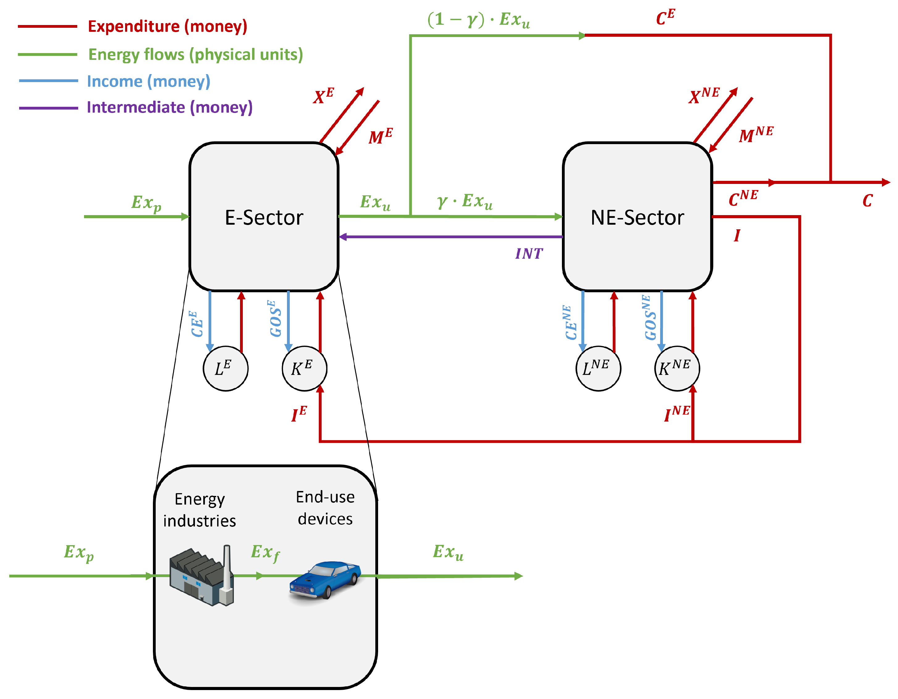
The E-Sector under the methodology we will be using goes beyond the traditional energy industries, encompassing every single physical process involved in the transformation of primary energy (extracted from the environment and including the extraction itself), into final energy (the final output of the traditional energy industries) and into the useful energy (measured as exergy) actually used to perform a given end-use in the economy. This includes not only the machines used in the traditional energy industries, such as boilers and turbines in a coal-fired power plant, but also devices used in households and firms, such as appliances, vehicles and computers. The output from this E-Sector corresponds to the useful exergy flows used to perform economic activities and generate economic value.
As we can see in Figure 1, exergy enters the economy through the E-Sector at the primary stage ( E x p ) and is transformed into its final stage ( E x f ) in traditional energy industries and then into its useful stage ( E x u ) by end-use devices. The production of useful exergy output from the E-Sector is powered by capital and labour inputs to this sector ( K E and L E , respectively) in exchange for payments to capital, known as “gross operating surplus”, and payments to labour, known as “compensation of employees” ( G O S E and C E E , respectively).
The useful exergy output from the E-Sector will be either used as an input in the production of non-energy goods and services in the NE-Sector ( 0 < γ < 1 ), alongside inputs of capital and labour to this sector ( K N E and L N E , respectively, paid for through G O S N E and C E N E , respectively) and in exchange for an intermediate consumption payment from the NE-Sector to the E-Sector ( I N T ), or consumed directly by households and government ( 1 γ ) through their expenditure on energy-converting goods and services ( C E ). This exchange of exergy for money between the E-Sector and the households and government is represented in the diagram by the point where the green arrow ( 1 γ ) E x u transforms into the red arrow C E . The output from the NE-Sector constitutes either consumption expenditure of non-energy goods and services ( C N E ) or investment expenditure allocated between the NE-Sector and the E-Sector ( I N E and I E , respectively).
Both the E-Sector and the NE-Sector also take into account the trade balance between exports ( X E and X N E , respectively) and imports ( M E and M N E , respectively).

2.2. Reclassification of National Accounts

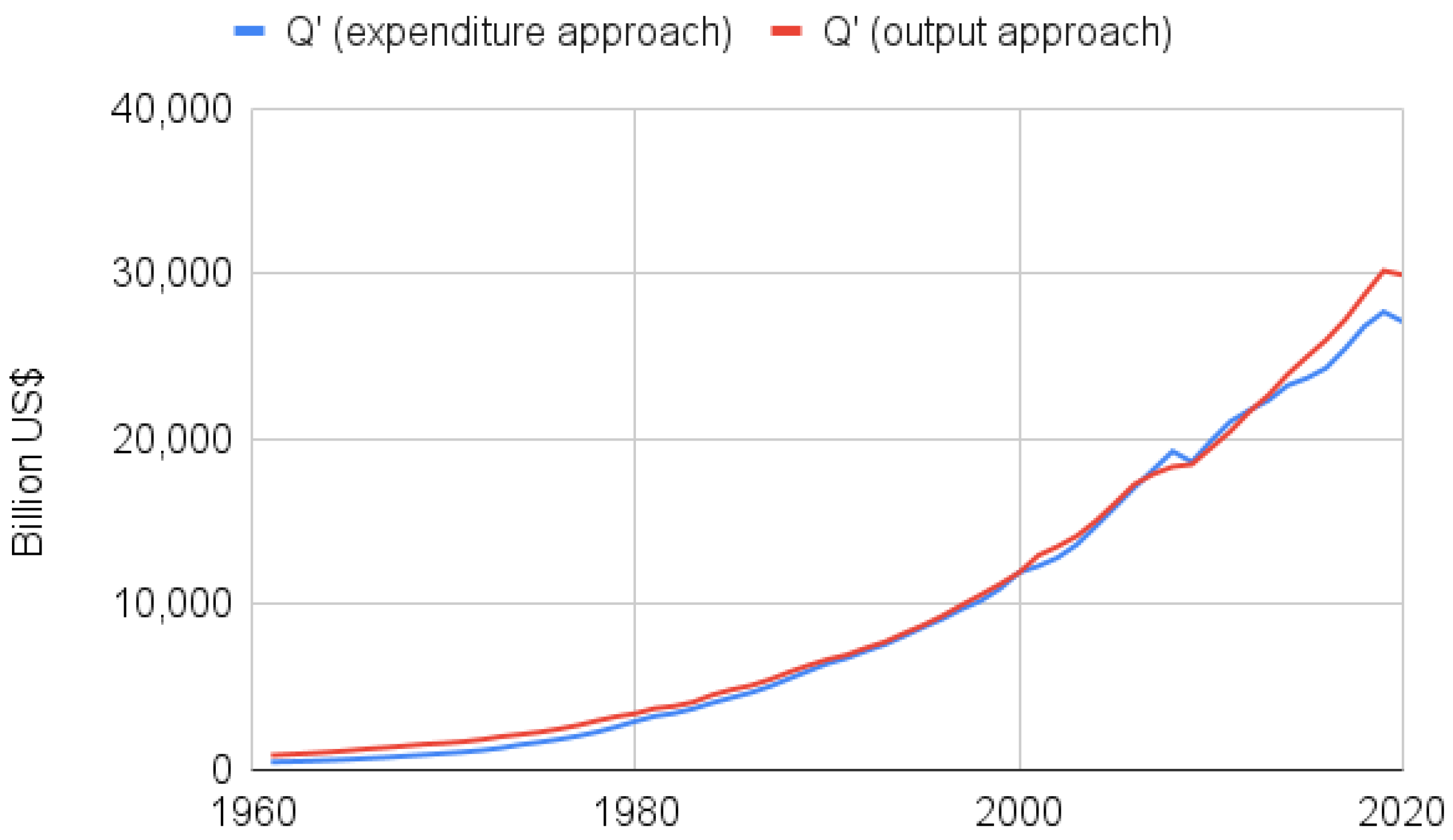
The central identity in national accounts expressed by Equation (1) equates the economic output (i.e., the Gross Domestic Product or GDP, represented by Q), calculated through the income approach, with the economic output calculated through the expenditure approach [21].
C + I + X M = Q = G O S + C E + ( T S ) P
In Equation (1), the l.h.s. (expenditure approach) represents the sum of consumption (C), investment (I) and the trade balance between exports (X) and imports (M), while the r.h.s. (income approach) represents the sum of payments to capital, measured as gross operating surplus ( G O S ), payments to labour, measured as compensation of employees ( C E ) and taxes minus subsidies on production and imports, ( T S ) P .
In the two-sector model, each term in Equation (1) is disaggregated in an E-Sector and an NE-Sector component, according to the previously established criteria for these sectors. In particular, this means that investment, exports and imports in energy-related goods and industries are allocated to the E-Sector, while investment, exports and imports in all other goods and industries are allocated to the NE-Sector. This reclassification, however, takes into account the fact that expenditure in energy-converting end-use devices (such as appliances) that is listed in national accounts as consumption is actually a form of investment expenditure in the E-Sector under our two-sector model, and so it is reclassified as such, while its associated imputed rents—estimated from average depreciation—are added to consumption expenditure. This is because consumption expenditure on energy-converting end-use devices contributes to the E-Sector’s capacity to generate useful exergy from final exergy. The consumption of energy-carriers is also allocated to the E-Sector, while the consumption of non-energy-converting goods is allocated to the NE-Sector. A similar disaggregation is employed for G O S , C E and ( T S ) P , leading to the equality in Equation (2) from Santos et al. [18].
( C E + C N E ) + ( I E + I N E ) + ( X E + X N E ) ( M E + M N E ) = Q = ( G O S E + G O S N E ) + ( C E E + C E N E ) + ( ( T E S E ) P ( T N E S N E ) P )
As was the case for Q in Equation (1), Q in Equation (2) represents the total economic output. This will be different from GDP as reported in national accounts because it will include the imputed rents associated with the reclassification of consumption expenditure as investment on the l.h.s, but since it will also include its respective payments to capital (which have the same value) on the r.h.s, the equality still holds.
A detailed diagram of the extended energy sector is presented in Figure 2. Following the Statistical Classification of Economic Activities in the European Community (NACE, from the French “Nomenclature statistique des Ativités économiques dans la Communauté Européenne”), the industry standard classification system used in the European Union, this E-Sector is made up of the traditional energy sector (NACE categories “Mining & quarrying” and “Electricity, gas, steam & AC supply”) and supplementary economic activities ultimately responsible for energy transformation but not typically classified as part of the energy sector (NACE categories “Agriculture, forestry & fishing”, “Manufacture of food, beverages, & tobacco products” and “Manufacture of coke & refined petroleum products”).
The gross value added ( G V A E ) of both the conventional and these supplementary economic activities, combined with the value of the end-use devices converting exergy at the final-to-useful stage ( G V A I m p E ), forms the total GVA for the extended energy sector ( G V A E ).
In addition to the identity expressed in Equation (2), the disaggregation and reclassification of national accounts in the two-sector model must satisfy the sector-specific accounting identities illustrated in the circular flow diagram of Figure 3.
These identities can be represented by the following equations from Santos et al. [18]:
  • Households:
    P N E + P E + S a v + ( T S ) H = G O S N E + C E N E + G O S E + C E E
  • Government:
    G N E + G E + Δ G o v = ( T S ) H + ( T S ) P N E + ( T S ) P E
  • Banks:
    N E L + N I L N E + N I L E = S a v + Δ G o v
  • Rest of the world (ROW):
    ( X N E M N E ) + ( X E M E ) = N E L
  • Firms (E):
    G O S E + C E E + ( T S ) P E + I E = P E + G E + N I L E + ( X E M E ) + I N T
  • Firms (NE):
    G O S N E + C E N E + ( T S ) P N E + I N T = P N E + G N E + N I L N E + ( X N E M N E ) + I E
For Equations (3)–(8), the l.h.s represents money flows going out of that specific sector while the r.h.s represents money flows going into that specific sector.
P N E and P E represent private consumption expenditure made by the Households in the NE-Sector and the E-Sector, respectively, S a v represents Household savings (which will go to the Banks) and ( T S ) H represents taxes minus subsidies on household consumption (which will be paid to the Government).
G O S N E is the gross operating surplus of the NE-Sector and C E N E is the compensation of employees in the NE-Sector. Together, these two factors, which come from Firms (E) (Equation (7)), make up the gross value added (GVA) of the NE-Sector, which reverts back to the Households. The same is true for the gross operating surplus and the compensation of employees in the E-Sector ( G O S E and C E E , respectively), which make up the GVA of the E-Sector and come from Firms (NE) (Equation (8)).
Similarly, on the r.h.s of Equation (4), in addition to the taxes minus subsidies from the Households, ( T S ) P N E (taxes minus subsidies from production in the NE-Sector) and ( T S ) P E (taxes minus subsidies from production in the E-Sector) are paid to the Government and are spent on G N E and G E (government consumption in the NE-Sector and the E-Sector, respectively). The balance between income to the Government and expenses by the Government, Δ G o v , is the government surplus (which will go to the Banks).
The Banks spend the savings and government surplus money they receive from the Households and the Government in N E L (net external lending to the rest of the world, or ROW), N I L N E (net internal lending to the NE-Sector) and N I L E (net internal lending to the E-Sector).
In the trade balance of Equation (6), on the l.h.s., X N E and X E are the exports in the NE-Sector and in the E-Sector, respectively, and M N E and M E are the imports in the NE-Sector and in the E-Sector, respectively.
In addition to the payments to capital and labour and the taxes minus subsidies on production, which both Firms in the E-Sector (Equation (7), l.h.s.) and in the NE-Sector (Equation (8), l.h.s.) pay to their specific sector, Firms in the E-Sector also invest in the NE-Sector ( I E ) in exchange for a payment in intermediate consumption ( I N T ). Both sectors are financed by private and government consumption, as well as net internal lending and trade balance.

2.3. Expenditure Approach

Each of the expenditure approach terms in Equation (1) was disaggregated into an E-Sector component and an NE-Sector component, as can be seen in Equation (2). The criteria for this disaggregation will be explained for each of these components in the following sections.
National accounts data were collected throughout this work from databases and official sources. The sources for the datasets used can be seen in Table A1 in Appendix A. Each data entry was allocated to either the E-Sector or the NE-Sector according to the criteria outlined in the following sections.

2.3.1. Consumption

The total consumption expenditure (C) is the sum of private (P) and government (G) consumption expenditure. Each of these subcomponents of consumption expenditure is disaggregated, in most databases, by type of good or purpose.
The Classification of Individual Consumption According to Purpose (COICOP) is a classification system for individual consumption expenditures published by the United Nations Statistics Division (UNSD). It is structured in four levels: Divisions (two-digit), Groups (three-digit), Classes (four-digit) and Subclasses (five-digit). COICOP data for private expenditure will be used in this work at the three-digit level. A detailed list of all COICOP Divisions and Groups is presented in Appendix B.1.
For government expenditure, the classification system used by the UNSD is the Classification of the Functions of Government (COFOG), which follows a structure similar to that of COICOP. COFOG data for government expenditure will be used in this work at the three-digit level. A detailed list of all COFOG Divisions and Groups is presented in Appendix B.2.
Annual time series for aggregate private (P) and government (G) consumption for the USA in the period 1960–2020 were obtained from the AMECO database [22] with nominal value.
Annual time series for disaggregate private consumption for the USA in the period 1960–2020 were obtained from the Bureau of Economic Analysis (BEA) [23] with nominal value. A correspondence was established between the BEA categories and those of COICOP. This correspondence can be seen in Appendix B.3. The time series for each category in this dataset was then allocated to either the E-Sector or the NE-Sector according to the rule established in Table A2, Appendix A. The consumption data in Division 1 (“Food and non-alcoholic beverages”), for example, were allocated to the E-Sector, as per Table A2, while the consumption data in Division 3 (“Clothing and footwear”), for example, were allocated to the NE-Sector, again as per Table A2.
Annual time series for disaggregate government consumption for the USA in the period 1970–2020 were obtained from the Organisation for Economic Co-operation and Development (OECD) database [24] in COFOG categories, but only at the Division level. The time series for each category in this dataset was allocated to either the E-Sector or the NE-Sector according to the rule established in Table A3, Appendix A, similarly to what was carried out in the case of private consumption. For cases where a given Division included Groups corresponding to multiple variables, a decision was made to attribute 1 / N of the total expenditure in the Division to each Group within it, with N being the total number of Groups within the Division. For instance, as Division 4 (“Economic affairs”) includes a Group allocated to G N E and another Group allocated to I E ( G ) , 50% of government consumption in Division 4 was allocated to G N E and the remaining 50% was allocated to I E ( G ) .
The correspondence between disaggregate COICOP and COFOG consumption expenditure categories and each of the two-sector model’s variables is established according to the following criteria:
  • Expenditure on any type of energy-carrier good (e.g., food, fuels, electricity) is classified as consumption expenditure in the E-Sector ( P E , G E );
  • Expenditure on any type of non-energy related good or service (e.g., clothing, services) is classified as consumption expenditure in the NE-Sector ( P N E , G N E );
  • Expenditure on any type of good that actively participates in the conversion of final-to-useful exergy (e.g., vehicles, domestic appliances) is reclassified as investment expenditure in the E-Sector ( I E ( P ) , I E ( G ) ).
The reclassification of consumption expenditure on energy-converting goods as investment expenditure in the E-Sector is explained by the fact that these consumer goods are, in fact, acting in the economy to improve the E-Sector’s capacity to generate useful exergy from final exergy, meaning that their purchase constitutes an investment expenditure in the E-Sector to increase its useful exergy output. There will be imputed rents associated with this investment, which will be added to the private consumption expenditure in the E-Sector ( C I m p E ). These imputed rents will be equal to the gross operating surplus corresponding to each of these reclassified investment expenditure categories (see Section 3.2.4), thus representing their gross value added to the E-Sector ( G V A I m p E , see Section 2.2):
C I m p E = G O S I m p E = G V A I m p E
Table A2 and Table A3 show the correspondence between COICOP/COFOG expenditure categories and the two-sector model’s variables, respectively. For cases in which a given COICOP or COFOG category might contain goods corresponding to more than one of the two-sectors’ variables, a decision is made to split that category in half.
After disaggregating consumption expenditure, we end up with the following identity, where C is the total consumption expenditure in the two-sector model:
C = C E + C N E
With
C E = P E + G E + C I m p E
And
C N E = P N E + G N E

2.3.2. Investment

Investment expenditure is measured in national accounts as gross fixed capital formation (GFCF) and is generally disaggregated by type of asset. The breakdown of GFCF by type of asset used by the United Nations’ System of National Accounts (SNA) is shown in Table A4. GFCF data can also sometimes be found disaggregated by sector according to the Statistical Classification of Economic Activities in the European Community (NACE). A list of NACE categories is presented in Appendix B.4.
Annual time series for aggregate GFCF for the USA in the period 1960–2020 were obtained from the AMECO database [22] with nominal values.
Annual time series for GFCF disaggregated by type of asset according to Table A4 and by sector according to Table A5 were obtained for the USA for the years 1995–2020 from the Vienna Institute for International Economic Studies (wiiw, from the German “Wiener Institut für Internationale Wirtschaftsvergleiche”) [25].
The correspondence between disaggregate GFCF investment expenditure categories and each of the two-sector model’s variables is established according to the following criteria:
  • Expenditure on any type of asset that actively participates in the conversion of final-to-useful exergy (e.g., transport, machinery) is classified as investment expenditure in the E-Sector ( I E ( G F C F ) );
  • All expenditure on a sector that actively participates in the conversion of final-to-useful exergy (e.g., agriculture, forestry and fishing, coke and refined petroleum products) is classified as investment expenditure in the E-Sector ( I E ( G F C F ) ), regardless of asset type.
  • Expenditure on any type of asset that does not actively participate in the conversion of final-to-useful exergy and is not in a sector that actively participates in the conversion of final-to-useful exergy (e.g., research and development in the construction sector) is classified as investment expenditure in the NE-Sector ( I N E ).
The reclassification of all investment expenditure on energy-converting sectors as investment expenditure in the E-Sector, regardless of asset type, is explained by the fact that all investment in these sectors ultimately contributes to their goal of generating useful exergy from final energy/exergy.
Table A4 in Appendix A shows the correspondence between asset type expenditure categories and the two-sector model’s variables. For cases in which a given category might contain expenditure corresponding to more than one of the two-sector model’s variables, an estimate of how much of that category contributes to each variable is made using other economic data (see Section 3.1.2). Table A5 in Appendix A shows the correspondence between NACE categories and the two-sector model’s variables.
Finally, we must add to the investment expenditure in the E-Sector the reclassified consumption expenditure in this sector from Section 2.3.1, and so the total investment expenditure in the two-sector model ( I ) is given by
I = I N E + I E
With
I E = I E ( G F C F ) + I E ( P ) + I E ( G )

2.3.3. Exports and Imports

Exports and imports are usually disaggregated between goods and services. Exported and imported goods can also be found further disaggregated by type of good. One such form of disaggregation is the World Integrated Trade Solution (WITS), whose categories can be seen in Table A6 in Appendix A.
Annual time series for aggregate exports (X) and imports (M) for the USA in the period 1960–2020 were obtained from the AMECO database [22] with nominal values.
Annual time series for exports and imports disaggregated by WITS categories were obtained from the World Bank for the period 1991–2020.
The correspondence between disaggregate export and import categories and each of the two-sector model’s variables is established according to the following criteria:
  • Any type of energy-carrier good (e.g., food products, fuels) is classified as an export/import from/to the E-Sector.
  • Any type of non-energy-related good (e.g., footwear, metals) is classified as an export/import from/to the NE-Sector.
  • Any service is classified as an export/import from/to the NE-Sector.
Table A6 in Appendix A shows the correspondence between WITS categories and each of the two-sector model’s variables.

2.4. Factors of Production

2.4.1. Capital

Capital stocks for a given year t ( K t ) and for a given asset type are computed from the capital stock of that asset type in the previous year ( K t 1 ), the investment in that asset type in the present year ( I t ) and the consumption of fixed capital of that asset type in the present year ( C F C t ) according to the perpetual inventory method (PIM) [21] described by Equation (15).
K t = K t 1 + I t C F C t
C F C t is also given by the capital stock of the previous year multiplied by a (generally assumed to be constant) depreciation rate d, allowing us to rewrite Equation (15) as follows:
K t = K t 1 + I t d K t 1
In order to employ Equation (15), an initial value of capital stock must be provided. To achieve this, we will be using a common method found in the literature called “the steady-state approach”, given by Equation (17), where g G D P corresponds to the GDP growth rate averaged over the first three years in the sample.
K t 1 = I t g G D P + d
After the initial value of capital stock is calculated for each asset type, Equation (16) is used to calculate the capital stock of each asset type for the following years.
Annual time series for capital stocks disaggregated by asset type and sector were calculated using the PIM method and the GFCF dataset from Section 3.1.2. Depreciation rates were obtained from wiiw [25] and can be seen in Table A7.
The newly defined investment expenditure components, reclassified from expenditure traditionally allocated to consumption in national accounts, are labelled according to their corresponding asset-type categories. For instance, COICOP Division 7 Group 1, “Purchase of vehicles”, is included in asset-type category “Transport equipment (TraEq)”. Its corresponding initial capital stock and capital stock time series were then determined through Equation (16), using the corresponding depreciation rate from Table A7. The same was carried out for all other investment expenditure components reclassified from expenditure allocated to consumption in national accounts.

2.4.2. Labour

Labour inputs to production can be measured as the number of engaged individuals or as the number of hours worked by engaged individuals. Annual time series for both of these can be found for full-time and part-time employees in the USA by industry in either the Standard Industrial Classification (SIC) or the North American Industry Classification System (NAICS).
Annual time series for aggregate values of number of employees and self-employed individuals for the USA in the period 1960–2020 were obtained from the AMECO database [22].
Annual time series for disaggregate number of full-time and part-time employees by sector for the USA in the period 1960–2020 were obtained from the Bureau of Economic Analysis (BEA) [26]. In the period 1960–2000, the dataset is in the SIC classification system, while in the period 2001–2020 it is in the NAICS classification system. The correspondence between these categories and the two-sector model’s variables is established in Table A8 and Table A9, respectively.
Annual time series for the hours worked by full-time and part-time employees by sector for the USA in the period 1960–2020 were obtained from BEA [27]. Just as with the number of full-time and part-time employees, this dataset was in the SIC classification system in the period 1960–2000 and in the NAICS classification system in the period 2001–2020. However, this dataset had lower granularity than the dataset for number of employees and so some assumptions had to be made. The hours worked in the “Mining” and “Manufacturing/Nondurable goods” sectors from Table A8 and Table A9 were not disaggregated, and so we assumed that the percentages of work hours in these sectors allocated to the E-Sector and the NE-Sector would be the same as the percentages of full-time and part-time employees in these sectors working in the E-Sector and the NE-Sector, respectively. For example, in 1960, 30% of the workers in “Mining” were working in activities allocated to the NE-Sector, so the amount of hours worked in “Mining” activies in the NE-Sector in that year was calculated multiplying the total amount of work hours in “Mining” in 1960 by 30%. The same was carried out for every other year in the time series.
Annual time series for the number of self-employed individuals by sector for the USA in the period 1960–2020 were obtained from the BEA [28]. Just as with the number of full-time and part-time employees, this dataset was in the SIC classification system in the period 1960–2000 and in the NAICS classification system in the period 2001–2020. The number of hours worked by each self-employed person was calculated assuming that the number of hours worked per worker in a given year and sector is the same whether they are self-employed or employees.
Annual time series for compensation of employees disaggregated by sector for the USA in the period 1987–1997 were obtained from the BEA [29]. This dataset was in the NAICS classification system.
The correspondence between SIC/NAICS industries and each of the two-sector model’s variables is established according to the following criteria:
  • The E-Sector encompasses traditional energy industries, as well as other industries that participate actively in the conversion of primary-to-final-to-useful exergy in the economy;
  • The NE-Sector is constituted by the remaining activities.
This is illustrated in Figure 2, where we can see that the E-Sector encompasses conventional energy industries (NACE categories “Mining & quarrying” and “Electricity, gas, steam & AC supply”), supplement industries (NACE categories “Agriculture, forestry & fishing”, “Manufacture of food, beverages & tobacco products” and “Manufacture of coke & refined petroleum products”) and end-use devices, while the NE-Sector encompasses everything else.

2.5. Income Approach

Each of the income approach terms in Equation (1) was disaggregated into an E-Sector component and a NE-Sector component, as can be seen in Equation (2). The criteria for this disaggregation will be explained for each of these terms in the following sections.

2.5.1. Gross Operating Surplus

Payments to capital inputs to production are accounted for in national accounts as gross operating surplus ( G O S ). G O S is generally reported only at the aggregate level, and so disaggregate G O S by type of asset and by sector has to be estimated assuming that the share of G O S for each asset type and sector is equal to the share of CFC for those same asset types and sectors. G O S i j for asset type i and sector j was thus calculated using Equation (18), where N is the total number of asset types (listed in Appendix A, Table A4) and M the total number of sectors (listed in Appendix B.4).
G O S i j = j M i N G O S i j C F C i j j M i N C F C i j
The approach represented by Equation (18) is used only to estimate G O S corresponding to investment expenditure categories from GFCF. For investment expenditure reclassified from consumption expenditure in the two-sector model, the approach used is to straightforwardly equate the G O S with the corresponding CFC for these categories. The allocation of G O S according to payments to capital in the E-Sector and the NE-Sector of the two-sector model is carried out according to the same rule as the one used for investment expenditure (see Section 2.3.2).

2.5.2. Compensation of Employees

Payments to labour inputs to production are accounted for in national accounts as compensation of employees ( C E ), which, in this model, includes both payments to full-time and part-time employees ( C E e m p ) and to the self-employed ( C E s e ).
Compensation of employees can be found disaggregated by sector (SIC/NAICS) for full-time and part-time employees, but not for the self-employed. The payments to the self-employed were thus estimated by assuming that, for each sector, the average hourly compensation of the self-employed is equal to the average hourly compensation of the full-time and part-time workers.

2.5.3. Taxes Minus Subsidies on Production and Imports

Taxes minus subsidies on production and imports are usually reported only at the aggregate level. In this work, we assume that the proportion of aggregate taxes minus subsidies on production and imports allocated to each of the two sectors, E-Sector and NE-Sector, is the same as the share of gross value added (GVA) estimated for each sector, in terms of the total GVA for the whole economy. Since the GVA for each sector is given by the sum of the payments to capital and labour corresponding to that sector, the share of taxes minus subsidies on production and imports allocated to each sector will be:
( T S ) P k = G O S k + C E k G O S N E + C E N E + G O S E + C E E ( T S ) P , k = E , N E

2.6. Final and Useful Exergy Balances

Besides components from national macroeconomic accounts, exergy flows were also disaggregated and allocated to the two-sector model’s variables, namely at their final and useful stages.
Exergy balances disaggregated by sector are available for the USA. In our work, we will be focusing on the useful stage and the final-to-useful conversion of exergy flows, and so we will also consider the disaggregation of exergy balances by (useful) end-use in the economy. We adopt the useful exergy accounting procedure developed in Serrenho et al. [30]:
  • Conversion of existing final energy data to final exergy values;
  • Allocation of final exergy of each final use sector to useful exergy categories;
  • Calculation of overall useful exergy by summing the total values from each useful exergy category.
In the approach by Serrenho et al. [30], useful exergy (U) is calculated for each year (t), energy carrier (i), economic sector (j) and end-use category (k) with Equation (20), where ϵ t , k is the thermodynamic second-law efficiency for each end-use, ϕ i is an exergy factor (defined as the ratio of exergy to energy in the form of enthalpy, internal energy or others) and E t , i j k is final energy consumption data.
U t , i j k = ϵ t , k ϕ i E t , i j k
Annual time series data on the flows of final and useful exergy disaggregated by sector are taken directly from the useful work accounting procedure performed in the Country-Level Primary-Final-Useful (CL-PFU) database [31], which extends the International Energy Agency (IEA) World Extended Energy Balance data from the final energy stage to the useful exergy stage. This database includes exergy flow data from more than 150 different countries, disaggregated by sector and final energy carrier, for the period 1960–2020. We will use the data related to the US.
The correspondence between traditional institutional sectors, two-sector model sectors and end-uses can be seen in Table A12 in 
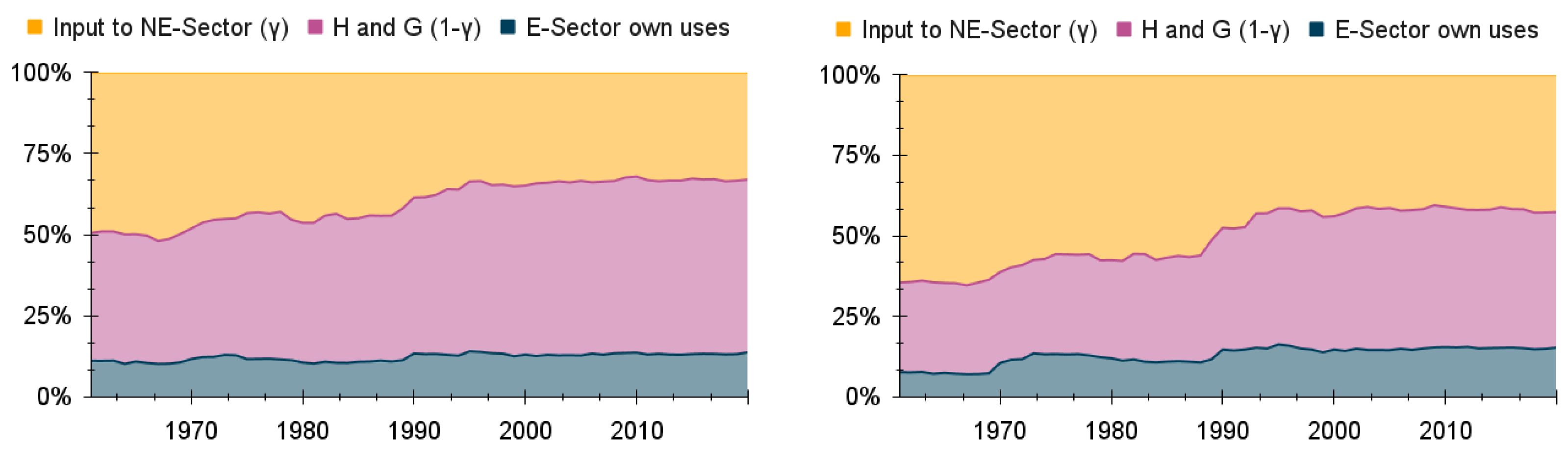
Appendix A. Once final/useful exergy balances are disaggregated according to this approach, they are allocated to the following components:
  • E-Sector own-uses;
  • Inputs to production processes of the NE-Sector;
  • Direct consumption by households and government.
E-Sector own-uses correspond to all exergy consumption by the traditional energy sector (energy industry own-uses), as well as consumption by the “Agriculture and forestry” and “Food and tobacco” sectors. Part of the “Mining and quarrying” sector is also allocated to E-sector own-uses, in particular the share corresponding to coal mining and oil and gas extraction, as well as the fraction of the “Chemical and petrochemical” sector corresponding to coke and refined petroleum products.
The remaining final/useful exergy flows, excluding the E-Sector own-uses, correspond to the total output from the E-Sector, which is allocated either to inputs to production in the NE-Sector, or direct consumption.
The “Residential” and “Roads” sectors are allocated towards direct consumption, while every other sector within the E-Sector output is allocated as an input to the NE-Sector.

2.7. Model Validation

The framework employed in this work consists in the reclassification of data from national accounts and exergy flows. It is a different conceptualisation of the economy with only two sectors, but it respects the same general principles and obeys similar identities (namely Equations (2)–(8)).
The central identity in national accounts as expressed through Equation (2) must still hold, and thus it can be used as a test for self-consistency. This test is performed during the reclassification process itself. In Figure 4, we compare Q’ as calculated through the expenditure approach (the l.h.s. of Equation (2)) with Q’ as calculated through the output approach (the r.h.s. of Equation (2)).
Figure 4 shows that the two approaches to calculating Q’ give consistent results.

3. Results and Discussion

In the previous section, we went through the disaggregation and reclassification steps required to restructure the macroeconomic national accounts data and the exergy flows data for the US economy into our two-sector model framework. Our motivation for employing this framework was that it allows us to study the role energy flows play in economic production in a physically coherent way (namely, by dealing with energy in the form of useful exergy and treating it as an intermediate input to production).
The following section details the application of this method to the datasets specified in the previous section, as well as a discussion on what this reclassification of national accounts and exergy flows means economically. A summary of the datasets used throughout this work can be seen in Table A1 in Appendix A.

3.1. Expenditure Approach

3.1.1. Consumption

As government consumption expenditure disaggregated by COFOG categories was unavailable for the period 1960–1970, the shares of total government consumption expenditure (G) allocated directly to the E-Sector ( G E ), to the NE-Sector ( G N E ) and reclassified as investment in the E-Sector ( I E ( G ) ) had to be estimated. G N E was estimated by assuming that its growth rate in the period 1960–1970 was the same as that of G in the same period and G E was estimated by assuming that it was constant, as a percentage of G, and equal to its average value in the period 1970–2020. To estimate I E ( G ) , we simply subtracted G N E and G E from G.
In order to have a complete picture of consumption expenditure in the two-sector model, we must bring in the imputed rents corresponding to investment expenditure reclassified as consumption expenditure from national accounts ( C I m p E ) from Section 3.2.4. These are summed to the consumption expenditure on goods and services produced by the E-Sector.
Figure 5 shows the allocation of private and government expenditure, in national accounts, according to the two-sector model’s variables for consumption and investment expenditure.
Figure 6 shows the allocation of total consumption expenditure according to the two-sector model’s variables.
Of all consumption expenditure, as defined in national accounts, most is allocated to the NE-Sector. The same is true for both private and government consumption individually. The share of total consumption allocated to the E-Sector diminishes with time, while the share allocated to investments in the E-Sector is somewhat constant. Imputed rents steadily grew in share with time, reaching values of about 25% of total consumption expenditure at the end of the period.
This is qualitatively consistent with the results for Portugal found using a similar methodology in Santos et al. [18], although the increase in the share of imputed rents is more pronounced for the case of the US. This trend seems to suggest increasing investments in end-use devices, which is consistent with other studies focusing on exergy efficiency in the US. In particular, Brockway et al. [32] concludes that there has been a growing tendency in the period since 1960 for American consumers to invest in inefficient end-use appliances such as air conditioners and larger, faster accelerating cars.

3.1.2. Investment

In order to estimate GFCF by type of asset and sector for the period 1960–1995, we assumed that the percentage of total GFCF allocated for each asset type and sector in that period was a constant and equal to its average value for the period 1995–2020.
Once a complete, disaggregate dataset for GFCF by asset type and sector was obtained for the whole period 1960–2020, each investment asset was allocated to its respective variable in the two-sector model according to the criteria established in Section 2.3.2. Specifically, investment in asset types corresponding to I E ( G F C F ) according to Table A4 was allocated to this variable, regardless of sector, and investment in sectors corresponding to I E ( G F C F ) according to Table A5 was also allocated to this variable, regardless of asset type. Investment in asset types and sectors corresponding to I N E according to both Table A4 and Table A5 was allocated to this variable.
According to Table A5, NACE category B (“Mining and quarrying”) is split between I E ( G F C F ) and I N E . This split was made using the percentages of full-time and part-time employees in this sector working in the E-Sector and the NE-Sector (with the dataset from Section 3.2.2). For instance, in 1960, 30% of the full-time and part-time employees working in “Mining” were working in the NE-Sector, and so 30% of the investment in NACE category B was allocated to I N E , with the rest being allocated to I E ( G F C F ) .
Consumption expenditure reclassified as investment in the E-Sector in Section 3.1.1 was added to I E .
Figure 7 shows the allocation of GFCF, in national accounts, according to the two-sector model’s variables.
Of all investment expenditure as defined in national accounts, the majority (>75%) is allocated to the NE-Sector, although its share seems to be declining. When taking investment reclassified from consumption expenditure into account, the E-Sector receives a little less than 50% of the total investment at present.
These results are fairly consistent with the ones found in Santos et al. [18] for the case of Portugal.

3.1.3. Exports and Imports

In order to estimate the exports and imports for the period 1960–1991, we calculated the percentage of exports/imports allocated to the E-Sector and the NE-Sector for the period 1991–2020, as well as the growth rate of exports/imports in each of these sectors and in total for that time period. As the growth rate of total exports/imports was similar to that of exports/imports in the NE-Sector for 1991–2020, the growth rate of total exports/imports in the period 1960–1991 was taken as the growth rate of the NE-Sector in this period. The values of exports/imports obtained for the NE-Sector were then subtracted from the total exports/imports in 1960–1991 to obtain the exports/imports in the E-Sector in this period.
Once a complete, disaggregate dataset for exports and imports was obtained for the whole period 1960–2020, each category was allocated to its respective variable in the two-sector model according to the Table A6.
Figure 8 shows the allocation of exports and imports, as defined in national accounts, according to the two-sector model’s variables.
In both exports and imports the vast majority of expenditure is allocated to the NE-Sector. This is consistent with the results found in Santos et al. [18] for the case of Portugal.

3.2. Factors of Production

3.2.1. Capital

Once a complete, disaggregate dataset for capital stock by asset type and sector was obtained for the whole period 1960–2020, each category was allocated to its respective variable in the two-sector model according to the criteria established in Section 3.1.2. The same process was applied to the newly defined investment expenditure components reclassified from expenditure traditionally allocated to consumption in national accounts from Section 3.1.1. Table A10 and Table A11 establish a correlation between COICOP and COFOG categories, respectively, and GFCF categories.
Figure 9 shows the allocation of capital stock according to the two-sector model’s variables.
Although, currently, capital stock is allocated evenly between the E-Sector and the NE-Sector, the historical trend has been for the fraction allocated to the E-Sector to increase (when taking consumption expenditure reclassified as investment into account). This behaviour is consistent with Section 3.1.1 and with the results in Santos et al. [18] for the case of Portugal, although in the case of the US, the increase in capital stock from consumption expenditure reclassified as investment is much more pronounced. This could be indicative of differences in consumer behaviour between these two countries, but it could also just be symptomatic of the US’s economic development having happened sooner than Portugal’s, leading to its increase in consumption of energy-converting appliances having happened sooner as well.

3.2.2. Labour

Once complete, disaggregate datasets for number of self-employed individuals, full-time and part-time employees, hours worked by self-employed individuals and hours worked by full-time and part-time employees were obtained for the whole period 1960–2020, each category was allocated to its respective variable in the two-sector model according to Table A8 and Table A9.
Figure 10 shows the allocation of full-time/part-time employees and the self-employed according to the two-sector model’s variables.
Figure 11 shows the allocation of work hours according to the two-sector model’s variables.
The vast majority of workers are full-time/part-time employees and, among those, the majority works in the NE-Sector. The number of total workers in the E-Sector has diminished with time. The same trends are true for work hours and both these results are qualitatively consistent with Santos et al. [18].
This reduction in the relative importance of employment in the E-Sector could be indicative of a natural shift of workers away from the agricultural and other related sectors and into the service industry as the economy of the US grew and developed with time.

3.2.3. Compensation of Employees

In order to estimate compensation of employees for the time periods 1960–1987 and 1997–2020, we assumed that the growth rate of compensation per employee for each sector was constant during these periods and equal to its average value in the period 1987–1997. With that, and the number of full-time and part-time employees, we calculated the compensation per employee for those years and for each sector. With those values and the number of self-employed individuals, and assuming that, for the same sector, the average compensation per hour is the same for full-time/part-time employees and self-employed individuals, we calculated the compensation of the self-employed.
Once complete, disaggregate datasets for compensation of employees, both full-time/part-time and self-employed, were obtained for the whole period 1960–2020, each category was allocated to its respective variable in the two-sector model according to Table A9.
Figure 12 shows the allocation of compensation of employees according to the two-sector model’s variables.
Just as with the number of workers and the number of work hours, the largest share of the total compensation of employees is allocated to the NE-Sector.

3.2.4. Gross Operating Surplus

The gross operating surplus ( G O S ) for each asset type and sector was calculated using the investment data from Section 3.1.2 and Equation (18), where CFC for each asset type was calculated by multiplying its stock in the previous year by its depreciation rate (Table A7).
For the investment in the E-Sector reclassified from consumption expenditure, CFC was taken as the value of G O S directly. This G O S also gives us the imputed rents associated with these investments, which were then added to the private consumption expenditure in the E-Sector in Section 3.1.1.

3.2.5. Taxes Minus Subsidies on Production and Imports

The allocation of taxes minus subsidies on production and imports between the E-Sector and the NE-Sector was established (Figure 13) according to the procedure established in Section 2.5.3 and using Equation (19).
Most taxes minus subsidies on production and imports are allocated to the NE-Sector, but the fraction allocated to the E-Sector is increasing.

3.3. Final and Useful Exergy Balances

The allocation of final/useful exergy flows to the E-Sector’s own-uses ( E x f O U , E x u O U ), inputs to the NE-Sector ( γ ) and direct consumption by households and government ( 1 γ ) was established according to the procedure presented in Section 2.6 and summarised in Table A12 in Appendix A.
The share of the “Chemical and petrochemical” sector going into the E-Sector’s own-uses was estimated using the share of GVA the “Coke and refined petroleum products” industry represents within this sector. The share of the “Mining and quarrying” sector going into the E-Sector’s own-uses was estimated using the percentage of workers within this sector working in the E-Sector.
The allocation of final/useful exergy according to the two-sector model’s variables can be seen in Figure 14.
The share corresponding to the E-Sector’s own-uses remains relatively constant throughout the entire period. The input to the NE-Sector represented the largest share of the output of the E-Sector towards the beginning of the period, but there was a clear tendency for it to diminish throughout the second half of the last century, while the share of exergy going into household and government consumption grew. Since the turn of the century, these shares have been relatively constant.
These results are consistent with the ones obtained for the disaggregation of macroeconomic national accounts, in particular the ones relating to investment and capital stock, as they also show a relative increase in the importance of end-use devices (which, in this case, are included in the exergy used by households and the government).

4. Conclusions

In this work, we applied a two-sector model to the US economy that is consistent with energy’s role as an intermediate input in economic production. We also chose to treat energy flows in their most significant form, i.e., useful exergy, in contrast to the usual approaches found in the literature. Our goal was to study the relationship between exergy flows and economic development.
We analysed macroeconomic national accounts and exergy flow data for the US for the period 1960–2020, disaggregating and reclassifying them in terms of an extended energy sector and a non-energy sector.
Our analysis shows that the shares of consumption expenditure allocated to either the extended energy sector or the non-energy sector were relatively constant throughout the time period studied (Figure 5). The imputed rents associated with consumption reclassified as investment in the extended energy sector, however, grew steadily (Figure 6, right). This is consistent with the distribution of capital stock between the two sectors. While the shares of capital stock from traditional investment in either the extended energy sector or the non-energy sector remained relatively constant (Figure 9, left), the capital stock derived from consumption expenditure reclassified as investment in the extended energy sector increased considerably in the time period studied (Figure 9, right). This growth could be reflective of a tendency for the increased consumption of end-use devices (e.g., air conditioners or cars) among American consumers. As seen in Brockway et al. [32], the average exergy efficiency across all productive processes in the US economy remained relatively constant during the time period studied. This means that an increase in the consumption of end-use devices inevitably leads to increased overall exergy consumption.
This could either mean that useful exergy flows are a major driver of economic growth (which would be consistent with previous studies performed for the US economy in [3,10]) or that increased useful exergy consumption happens as a consequence of economic growth. Either way, this conclusion has important implications for economic policy, as the Integrated Assessment Models on which climate policy is based are either built upon neoclassical production functions (which often disregard the role of energy entirely) or they use energy as a primary (and not intermediate) factor of production [33,34,35]. This means that the relationship between economic growth and increased exergy consumption is being undervalued and it suggests that making economic development compatible with reducing energy demand is a problem that needs to be solved in a global economy with climate policies, as has already been pointed out in the literature (e.g., [34]).
When comparing these results with the ones for Portugal in Santos et al. [18], we see similar qualitative results, namely an increase in the shares of investment and capital stock going to the extended energy sector due to consumption expenditure reclassified as investment. Quantitatively, however, this increase is much more pronounced for the US. This could be due to differences in consumer habits, which, in turn, could either be cultural or reflective of the different stages of economic development the two countries were in during the time period considered, with the US’s economic development having happened sooner. Either way, with the US being the world’s leading economy by GDP, this effect being more pronounced for the US could have important economic and environmental consequences which need to be considered further.
Our analysis of labour and compensation of employees data is consistent with the hypothesis that these results showcase the earlier economic development of the US. While the shares of workers and of compensation of employees in the extended energy sector have clearly decreased for both the US and Portugal (Figure 10 and Figure 12), they were already much less significant for the US than for Portugal at the beginning of the time period considered. In the case of Portugal, the share of workers in the extended energy sector was considerable (more than 40%) in the beginning of the 1960–2014 time period, before decreasing rapidly to below 20%. The same is true for compensation of employees. For the US, both these variables were already below 20% at the beginning of this time period. This could be explained by the importance of the agricultural sector being much more pronounced in Portugal than in the US in 1960, which is, again, consistent with the later economic development of Portugal compared to the US.
The exergy flow disaggregation and reclassification seem to follow a similar trend, with the share of output from the extended energy sector going into household and government consumption increasing over time.
These results suggest a relationship between increased energy usage (namely, thanks to increasing investment in end-use devices that facilitate the transformation of final into useful exergy, in turn a result of the increased private consumption of these end-use devices) and economic development.
Nevertheless, in this study, we did not directly measure our results against economic growth data, and so the outcomes of this work beg further investigation. A possible future step would be to estimate useful exergy prices and see how they change with the historical evolution of GDP, namely by performing a growth accounting analysis using the two-sector model. With the US being the largest economy in the world by GDP, these studies could aid in the creation of a more physically consistent climate policy, which would be extremely useful considering the need to move away from fossil fuels and the limits to useful exergy usage imposed by a finite planet.

Author Contributions

Conceptualization: J.S., T.D. and J.G.; methodology: J.S., T.D. and J.G.; formal analysis: J.G.; resources: J.S., M.H., P.E.B. and T.D.; data curation: J.G., M.H. and P.E.B.; writing—original draft preparation: J.G.; writing—review and editing: J.G, J.S., M.H., P.E.B. and T.D.; funding acquisition: T.D. All authors have read and agreed to the published version of the manuscript.

Funding

This research was funded by the Portuguese Recovery and Resilience Program (PRR), IAPMEI/ANI/FCT, Blockchain.PT, Contract no. 51. This work was supported by FCT/MCTES (PIDDAC) through project LARSyS - FCT Pluriannual funding 2020-2023 (UIDB/EEA/50009/2020). We acknowledge support for P.E.B. under EPSRC Fellowship award EP/R024251/1.

Data Availability Statement

Sources for the national accounts datasets can be seen in Table A1 in Appendix A. Results regarding the CL-PFU database will be made available by the authors on request.

Conflicts of Interest

The authors declare no conflicts of interest.

Abbreviations

The following abbreviations are used in this manuscript:
BEABureau of Economic Analysis
CECompensation of Employees
CFCConsumption of Fixed Capital
COFOGClassification of the Functions of Government
COICOPClassification of Individual Consumption According to Purpose
CL-PFUCountry-Level Primary-Final-Useful
GDPGross Domestic Product
GFCFGross Fixed Capital Formation
GOSGross Operating Surplus
GVAGross Value Added
IEAInternational Energy Agency
NACEStatistical Classification of Economic Activities in the European Community
NAICSNorth American Industry Classification System
OECDOrganisation for Economic Co-operation and Development
SICStandard Industrial Classification
SNASystem of National Accounts
UNSDUnited Nations Statistics Division
WITSWorld Integrated Trade Solution

Nomenclature

The following nomenclature is used in this manuscript:
CConsumption
dDepreciation rate
E (as superscript)E-Sector
E x Exergy flow
f (as underscript)Final
GGovernment
g G D P GDP growth rate averaged over the first three years in the sample.
H (as underscript)Households
IInvestment
I N T Intermediate consumption from the NE-Sector to the E-Sector
KCapital
LLabour
MImports
N E (as superscript)NE-Sector
N E L Net external lending
N I L Net internal lending
PPrivate
P (as underscript)Production
p (as underscript)Primary
S a v Savings
SSubsidies
TTaxes
t (as underscript)Year
u (as underscript)Useful
XExports
Δ G o v Government surplus
γ Share of useful exergy output from the E-Sector used as input in the NE-Sector

Appendix A

Table A1. Datasets used throughout the work. All monetary quantities were converted to Billion USD during the analysis.
DescriptionUnitsSource
Aggregate private consumption 1960–2020Billion USD (nominal)AMECO [22]
Aggregate government consumption 1960–2020Billion USD (nominal)AMECO [22]
Disaggregate private consumption 1960–2020Billion USD (nominal)BEA [23]
Disaggregate government consumption 1970–2020Billion USD (nominal)OECD [24]
Aggregate GFCF 1960–2020Billion USD (nominal)AMECO [22]
Disaggregate GFCF 1995–2020Million USD (nominal)wiiw [25]
Aggregate exports 1960–2020Billion USD (nominal)AMECO [22]
Disaggregate exports 1991–2020Thousand USD (nominal)World Bank
Aggregate imports 1960–2020Billion USD (nominal)AMECO [22]
Disaggregate imports 1991–2020Thousand USD (nominal)World Bank
Full-time and part-time employees by sector 1960–2020PersonsBEA [26]
Full-time and part-time employee work hours 1960–2020HoursBEA [27]
Self-employed individuals 1960–2020PersonsBEA [28]
Compensation of employees 1987–1997Billion USD (nominal)BEA [29]
Final exergyTJCL-PFU database [31]
Table A2. Divisions and Groups of COICOP and their corresponding variable in the 2-sector model.
COICOPVariable
DivisionsGroups
01- P E
02-
03- P N E
041–4
5 P E
051, 3–5 I E ( P )
2, 6 P N E
061 I E ( P )
2–3 P N E
071 I E ( P )
2–3 P N E
081, 3
2 I E ( P )
091–2
3–6 P N E
10–12-
Table A3. Divisions and Groups of COFOG and their corresponding variable in the 2-sector model.
COFOGVariable
DivisionsGroups
01–03- G N E
041–2, 4
3 G E
5–650% G N E , 50% I E ( G )
05- G N E
061–3, 5–6
450% G N E , 50% I E ( G )
071
2–6 G N E
08–10-
Table A4. Breakdown of GFCF by type of asset used by the UN’s SNA.
GFCF by Asset-TypeVariable
ConstructionDwellings (RStruc) I N E
Other buildings and structures (OCon)
Transport equipment (TraEq) I E ( G F C F )
Metal products
and machinery
Intellectual property productsComputer software and databases (Soft_DB) I N E
Research and Development (RD)
Other (OIPP)
Other investmentOther machinery, equipment and weapons (OMach)
ICTComputer hardware (IT) I E ( G F C F )
Communication equipment (CT)
Table A5. NACE investment categories and their corresponding variable in the 2-sector model.
NACEVariable
A I E ( G F C F )
B I N E / I E ( G F C F )
C10-C18 I N E
C19 I E ( G F C F )
C20-C33 I N E
D I E ( G F C F )
E-U I N E
Table A6. WITS exports/imports categories and their corresponding variable in the 2-sector model.
WITSVariable
Animal X E / M E
Chemicals X N E / M N E
Food Products X E / M E
Footwear X N E / M N E
Fuels X E / M E
Hides and Skins X N E / M N E
Mach and Elec
Metals
Minerals
Miscellaneous
Plastic or Rubber
Stone and Glass
Textiles and Clothing
Transportation
Vegetable X E / M E
Wood X N E / M N E
Table A7. GFCF asset types and their corresponding depreciation rates.
GFCF Categoryd
Dwellings (RStruc)0.011
Other buildings and structures (OCon)0.032
Transport equipment (TraEq)0.189
Computer software and databases (Soft_DB)0.315
Research and Development (RD)0.200
Other intellectual property products (OIPP)0.131
Other machinery, equipment and weapons (OMach)0.131
Computer hardware (IT)0.315
Communication equipment (CT)0.115
Table A8. SIC labour sectors and their corresponding variable in the 2-sector model.
SIC CategoryVariable
Agriculture, forestry and fishing L E
MiningMetal mining L N E
Coal mining L E
Oil and gas extraction
Nonmetallic minerals, except fuels L N E
Construction
ManufacturingDurable goods
Nondurable goodsFood and kindred products
Tobacco manufactures
Textile mill products
Apparel and other textile products
Paper and allied products
Printing and publishing
Chemicals and allied products
Petroleum and coal products L E
Rubber and miscellaneous plastics products L N E
Leather and leather products
TransportationsRailroad transportation
CommunicationTelephone and telegraph
Electric, gas and sanitary services L E
Wholesale trade L N E
Retail trade
Finance, insurance and real estateBanking
ServicesHotels and other lodging places
Government
Table A9. NAICS labour sectors and their corresponding variable in the 2-sector model.
NAICS CategoryVariable
Agriculture, forestry, fishing and hunting L E
MiningOil and gas extraction
Mining, except oil and gas L N E
Support activities for mining
Utilities
Construction
Manufacturing Durable goods
Nondurable goodsFood and beverage and tobacco products
Textile mills and textile product mills
Apparel and leather and allied products
Paper products
Printing and related support activities
Petroleum and coal products L E
Chemical products L N E
Plastics and rubber products
Wholesale trade
Retail trade
Transportation and warehousing
Information
Finance and insurance
Real estate and rental and leasing
Professional, scientific and technical services
Management of companies and enterprises
Administrative and waste management services
Educational services
Health care and social assistance
Arts, entertainment and recreation
Accommodation and food services
Other services, except government
Government
Table A10. COICOP categories and their corresponding GFCF categories.
COICOP CategoryGFCF Category
05.3 Household appliancesOther machinery, equipment and weapons
(OMach)
05.4 Glassware, tableware and household utensils
05.5 Tools and equipment for house and garden
06.1 Medical products, appliances and equipment
07.1 Purchase of vehiclesTransport equipment (TraEq)
08.2 Telephone and telefax equipmentCommunication equipment (CT)
09.1 Audio-visual, photographic and information processing equipment
09.2 Other major durables for recreation and cultureOther machinery, equipment and weapons (OMach)
Table A11. COFOG categories and their corresponding GFCF categories.
COFOG CategoryGFCF Category
040: Economic affairs50% Transport equipment (TraEq), 50% Communication equipment (CT)
060: Housing and community amenitiesOther machienry, equipment and weapons (OMach)
070: Health
Table A12. Correspondence between traditional sectors, two-sector model sectors and end-uses of exergy flows. In the “Chemical and petrochemical” and the “Mining and quarrying” sectors, part of the exergy flow is allocated directly to the E-Sector and the rest is used as input to the NE-Sector.
Traditional Sector2-Sector Model SectorEnd-Use
Agriculture/forestryE-Sector-
Blast furnaces
Chemical and petrochemicalE-Sector/NE-SectorInput to the NE-Sector
Coal minesE-Sector-
Coke ovens
Commercial and public servicesNE-SectorInput to the NE-Sector
Construction
Domestic aviation
Domestic navigation
Final consumption not elsewhere specified
Food and tobaccoE-Sector-
Gas works
Industry not elsewhere specifiedNE-SectorInput to the NE-Sector
Iron and steel
Machinery
Main activity producer CHP plantsE-Sector-
Main activity producer electricity plants
Main activity producer heat plants
Mining and quarryingE-Sector/NE-SectorInput to the NE-Sector
Natural gas extractionNE-SectorInput to the NE-Sector
Non-ferrous metals
Non-metallic minerals
Oil extractionE-Sector-
Oil refineries
Paper, pulp and printingNE-SectorInput to the NE-Sector
Pipeline transport
RailHouseholds and government
Residential
RoadHouseholds and government
Textile and leather
Transport equipment
Transport not elsewhere specified
Wood and wood products

Appendix B

Appendix B.1. COICOP

COICOP for private consumption expenditure is structured as follows (at most 3-digit level):
  • 01—Food and non-alcoholic beverages;
  • 02—Alcoholic beverages, tobacco and narcotics;
  • 03—Clothing and footwear;
  • 04—Housing, water, electricity, gas and other fuels;
      
    04.1—Actual rentals for housing;
      
    04.2—Imputed rentals for housing;
      
    04.3—Maintenance and repair of the dwelling;
      
    04.4—Water supply and miscellaneous services relating to the dwelling;
      
    04.5—Electricity, gas and other fuels;
  • 05—Furnishing, household equipment and routine household maintenance;
      
    05.1—Furniture and furnishings, carpets and other floor coverings;
      
    05.2—Household textiles;
      
    05.3—Household appliances;
      
    05.4—Glassware, tableware and household utensils;
      
    05.5—Tools and equipment for house and garden;
      
    05.6—Goods and services for routine household maintenance;
  • 06—Health;
      
    06.1—Medical products, appliances and equipment;
      
    06.2—Out-patient services;
      
    06.3—Hospital services;
  • 07—Transport;
      
    07.1—Purchase of vehicles;
      
    07.2—Operation of personal transport equipment;
      
    07.3—Transport services;
  • 08—Communications;
      
    08.1—Postal services;
      
    08.2—Telephone and telefax equipment;
      
    08.3—Telephone and telefax services;
  • 09—Recreation and culture;
      
    09.1—Audio-visual, photographic and information processing equipment;
      
    09.2—Other major durables for recreation and culture;
      
    09.3—Other recreational items and equipment, gardens and pets;
      
    09.4—Recreational and cultural services;
      
    09.5—Newspapers, books and stationery;
      
    09.6—Package holidays;
  • 10—Education;
  • 11—Restaurants and hotels;
  • 12—Miscellaneous goods and services.

Appendix B.2. COFOG

COFOG classification for government consumption expenditure is structured as follows (at most 3-digit level):
  • 01—General public services;
  • 02—Defence;
  • 03—Public order and safety;
  • 04—Economic affairs;
      
    04.1—General economic, commercial and labour affairs;
      
    04.2—Agriculture, forestry, fishing and hunting;
      
    04.3—Fuel and energy;
      
    04.4—Mining, manufacturing and construction;
      
    04.5—Transport;
      
    04.6—Communication;
      
    04.7—Other industries;
      
    04.8—R&D economic affairs;
      
    04.9—Economic affairs, n.e.c.;
  • 05—Environmental protection;
  • 06—Housing and community amenities;
      
    06.1—Housing development;
      
    06.2—Community development;
      
    06.3—Water supply;
      
    06.4—Street lighting;
      
    06.5—R&D Housing and community amenities;
      
    06.6—Housing and community amenities, n.e.c.;
  • 07—Health;
      
    07.1—Medical products, appliances and equipment;
      
    07.2—Outpatient services;
      
    07.3—Hospital services;
      
    07.4—Public health services;
      
    07.5—R&D Health;
      
    07.6—Health, n.e.c.;
  • 08—Recreation, culture and religion;
  • 09—Education;
  • 10—Social protection;

Appendix B.3. Correspondence between COICOP and BEA Categories

The following list provides the 2-digit level categories of COICOP and the BEA categories that were allocated to each. The COICOP categories that are unlisted were either absent or had the same wording in the BEA structure.
  • 01—Food and non-alcoholic beverages;
      
    Food and nonalcoholic beverages purchased for off-premises consumption;
      
    Food produced and consumed on farms;
  • 02—Alcoholic beverages, tobacco, narcotics;
      
    Alcoholic beverages purchased for off-premises consumption;
      
    Tobacco;
  • 03—Clothing and footwear;
      
    Garments;
      
    Other clothing materials and footwear;
      
    Jewelry and watches;
  • 04.1—Actual rents for housing;
      
    Rental of tenant-occupied nonfarm housing;
      
    Group housing;
  • 04.2—Imputed rentals for housing;
      
    Imputed rental of owner-occupied nonfarm housing;
      
    Rental value of farm dwellings;
  • 04.4—Water supply and miscellaneous services relating to the dwelling;
      
    Water supply and sanitation;
  • 04.5—Electricity, gas and other fuels;
      
    Electricity and gas;
  • 05.1—Furniture and furnishings, carpets and other floor coverings;
      
    Furniture and furnishings;
  • 05.6—Goods and services for routine household maintenance;
      
    Household supplies;
  • 06.1—Medical products, appliances and equipment;
      
    Pharmaceutical and other medical products;
      
    Therapeutic appliances and equipment;
  • 07.1—Purchase of vehicles;
      
    New motor vehicles;
      
    Net purchases of used motor vehicles;
      
    Sports and recreational vehicles;
      
    Motor vehicle parts and accessories;
  • 07.2—Operation of personal transport equipment;
      
    Motor vehicle fuels, lubricants and fluids;
      
    Fuel oil and other fuels;
  • 08.2—Telephone and telefax equipment;
      
    Telephone and related communication equipment;
  • 08.3—Telephone and telefax services;
      
    Telecommunication services;
      
    Internet access;
  • 09.1—Audio-visual, photographic and information processing equipment;
      
    Video, audio, photographic and information processing equipment and media;
  • 09.2—Other major durables for recreation and culture;
      
    Sporting equipment, supplies, guns and ammunition;
      
    Musical instruments;
      
    Luggage and similar personal items;
  • 09.3—Other recreational items and equipment, gardens and pets;
      
    Recreational items;
  • 09.5—Newspapers, books and stationery;
      
    Recreational books;
      
    Magazines, newspapers and stationery;
  • 11—Restaurants and hotels;
      
    Accomodations;
      
    Food services;
  • 12—Miscellaneous goods and services;
      
    Personal care products;
      
    Net expenditures abroad by U.S. residents;
      
    Financial services and insurance;
      
    Professional and other services;
      
    Personal care and clothing services;
      
    Social services and religious activities;
      
    Household maintenance;
      
    Net foreign travel;
      
    Final consumption expenditures of nonprofit institutions serving households.

Appendix B.4. NACE Classification

The NACE classification is structured as follows (at most 2-digit level):
  • A—Agriculture, forestry and fishing;
  • B—Mining and quarrying;
  • C—Manufacturing
      
    C10—Manufacture of food products;
      
    C11—Manufacture of beverages;
      
    C12—Manufacture of tobacco products;
      
    C13—Manufacture of textiles
      
    C14—Manufacture of wearing apparel;
      
    C15—Manufacture of leather and related products;
      
    C16—Manufacture of wood and products of wood and cork, except furniture;
      
    C17—Manufacture paper and paper products;
      
    C18—Printing and reproduction of recorded media;
      
    C19—Manufacture of coke and refined petroleum products;
      
    C20—Manufacture of chemicals and chemical products;
      
    C21—Manufacture of basic pharmaceutical products and pharmaceutical preparations;
      
    C22—Manufacture of rubber and plastic products;
      
    C23—Manufacture of other non-metallic mineral products;
      
    C24—Manufacture of basic metals;
      
    C25—Manufacture of fabricated metal products, except machinery and equipment;
      
    C26—Manufacture of computer, electronic and optical products;
      
    C27—Manufacture of electrical equipment;
      
    C28—Manufacture of machinery and equipment n.e.c.;
      
    C29—Manufacture of motor vehicles, trailers and semi-trailers;
      
    C30—Manufacture of other transport equipment;
      
    C31—Manufacture of furniture;
      
    C32—Other manufacturing;
      
    C33—Repair and installation of machinery and equipment;
  • D—Electricity, gas, steam and air conditioning supply;
  • E—Water supply, sewerage, waste management and remediation activities;
  • F—Construction;
  • G—Wholesale and retail trade, repair of motor vehicles and motorcycles;
  • H—Transporting and storage;
  • I—Accommodation;
  • J—Information and communication;
  • K—Financial and insurance activities;
  • L—Real estate activities;
  • M—Professional, scientific and technical activities;
  • N—Administrative and support service activities;
  • O—Public administration and defense, compulsory social security;
  • P—Education;
  • Q—Human health and social work activities;
  • R—Arts, entertainment and recreation;
  • S—Other services activities;
  • T—Activities of households as employers, undifferentiated goods—and services—producing activities of households for own-use,
  • U—Activities of exterritorial organisations and bodies.

References

  1. Abramovitz, M. Resources and output trends in the United States since 1870. In Thinking about Growth: And Other Essays on Economic Growth and Welfare. Studies in Economic History and Policy: USA in the Twentieth Century; Cambridge University Press: Cambridge, UK, 1989; pp. 127–147. [Google Scholar]
  2. Solow, R.M. A contribution to the theory of economic growth. Q. J. Econ. 1956, 70, 65–94. [Google Scholar] [CrossRef]
  3. Warr, B.; Ayres, R.U. Useful work and information as drivers of economic growth. Ecol. Econ. 2012, 73, 93–102. [Google Scholar] [CrossRef]
  4. Santos, J.; Borges, A.S.; Domingos, T. Exploring the links between total factor productivity and energy efficiency: Portugal, 1960–2014. Energy Econ. 2021, 101, 105407. [Google Scholar] [CrossRef]
  5. Ayres, R.U. Green Economy Reader: Lectures in Ecological Economics and Sustainability; Springer: Cham, Switzerland, 2017; pp. 39–53. [Google Scholar]
  6. U.S. Bureau of Economic Analysis. Table 1.10. Gross Domestic Income by Type of Income. Available online: https://apps.bea.gov/iTable/?reqid=19&step=3&isuri=1&nipa_table_list=51&categories=survey (accessed on 20 January 2024).
  7. Platchkov, L.M.; Pollitt, M.G. The economics of energy (and electricity) demand. In The Future of Electricity Demand: Customers, Citizens and Loads; Cambridge University Press: Cambridge, UK, 2011; Volume 69. [Google Scholar]
  8. US Energy Information Administration. International Energy Outlook 2011; US Energy Information Administration: Washington, DC, USA, 2011.
  9. Warr, B.; Ayres, R.U. REXS: A forecasting model for assessing the impact of natural resource consumption and technological change on economic growth. Struct. Chang. Econ. Dyn. 2006, 17, 329–378. [Google Scholar] [CrossRef]
  10. Ayres, R.U.; Warr, B. REXS: Accounting for growth: The role of physical work. Struct. Chang. Econ. Dyn. 2005, 16, 181–209. [Google Scholar] [CrossRef]
  11. Warr, B.S.; Ayres, R.U. Evidence of causality between the quantity and quality of energy consumption and economic growth. Energy 2010, 35, 1688–1693. [Google Scholar] [CrossRef]
  12. Orecchini, F. The Era of Energy Vectors. Int. J. Hydrogen Energy 2006, 31, 1951–1954. [Google Scholar] [CrossRef]
  13. Eisenmenger, N.; Warr, B.; Magerl, A. Trends in Austrian Resource Efficiency: An Exergy and Useful Work Analysis in Comparison to Material Use, CO2 Emissions, and Land Use. J. Ind. Ecol. 2017, 21, 1250–1261. [Google Scholar] [CrossRef] [PubMed]
  14. Kümmel, R.; Lindenberger, D. How energy conversion drives economic growth far from the equilibrium of neoclassical economics. New J. Phys. 2014, 16, 125008. [Google Scholar] [CrossRef]
  15. D’Arge, R.C.; Kogiku, K.C. Economic Growth and the Environment. Rev. Econ. Stud. 1973, 40, 61–77. [Google Scholar] [CrossRef]
  16. Van den Bergh, J.C.; Nijkamp, P. Dynamic macro modelling and materials balance: Economic-environmental integration for sustainable development. Econ. Model. 1994, 11, 283–307. [Google Scholar] [CrossRef]
  17. Stern, D.I. Limits to substitution and irreversibility in production and consumption: A neoclassical interpretation of ecological economics. Ecol. Econ. 1997, 21, 197–215. [Google Scholar] [CrossRef]
  18. Santos, J.; Domingos, T.; Sousa, T.; Serrenho, A. Development of a Two-Sector Model with an Extended Energy Sector and Application to Portugal (1960–2014). MPRA 2018. Available online: https://ideas.repec.org/p/pra/mprapa/89175.html (accessed on 10 November 2023).
  19. Dincer, I.; Rosen, M.A. Chapter 4—Exergy, Environment And Sustainable Development. In Exergy: Energy, Environment and Sustainable Development, 2nd ed.; Elsevier: Amsterdam, The Netherlands, 2013; pp. 51–73. [Google Scholar]
  20. Reistad, G.M. Available Energy Conversion and Utilization in the United States. J. Eng. Gas Turbines Power 1975, 97, 429–434. [Google Scholar] [CrossRef]
  21. National Accounts: A Practical Introduction, Department of Economic and Social Affairs, Statistics Division, United Nations 2003. Available online: https://unstats.un.org/unsd/publication/seriesf/seriesf_85.pdf (accessed on 22 December 2023).
  22. AMECO. European Commission’s Annual Macro-Economic Database, Tables: 2.1—Private Final Consumption Expenditure; 2.5—Total Final Consumption Expenditure of General Government; 3.7—Gross Fixed Capital Formation by Type of Good at Current Prices; 9.1—Exports of Goods and Services; 9.2—Imports of Goods and Services. Available online: https://dashboard.tech.ec.europa.eu/qs_digit_dashboard_mt/public/sense/app/667e9fba-eea7-4d17-abf0-ef20f6994336/sheet/2f9f3ab7-09e9-4665-92d1-de9ead91fac7/state/analysis (accessed on 26 December 2023).
  23. Bureau of Economic Analysis (BEA). Available online: https://apps.bea.gov/iTable/?reqid=19&step=2&isuri=1&categories=survey (accessed on 26 December 2023).
  24. Organisation for Economic Co-operation and Development (OECD). Available online: https://data.oecd.org/ (accessed on 26 December 2023).
  25. Vienna Institute for International Economic Studies (wiiw, from the German “Wiener Institut für Internationale Wirtschaftsvergleiche”), “Statistical Capital for the US 1995–2020”. Available online: https://euklems.eu/archive-history/query-archive/ (accessed on 26 December 2023).
  26. Bureau of Economic Analysis (BEA), Tables 6.4A, 6.4B, 6.4C: Full-Time and Part-Time Employees by Industry. Available online: https://apps.bea.gov/iTable/?reqid=19&step=2&isuri=1&categories=survey#eyJhcHBpZCI6MTksInN0ZXBzIjpbMSwyLDNdLCJkYXRhIjpbWyJjYXRlZ29yaWVzIiwiU3VydmV5Il0sWyJOSVBBX1RhYmxlX0xpc3QiLCIxOTAiXV19 (accessed on 26 December 2023).
  27. Bureau of Economic Analysis (BEA), Tables 6.9B, 6.9C, 6.9D: Hours Worked by Full-Time and Part-Time Employees by Industry. Available online: https://apps.bea.gov/iTable/?reqid=19&step=2&isuri=1&categories=survey#eyJhcHBpZCI6MTksInN0ZXBzIjpbMSwyLDNdLCJkYXRhIjpbWyJjYXRlZ29yaWVzIiwiU3VydmV5Il0sWyJOSVBBX1RhYmxlX0xpc3QiLCIyMTAiXV19 (accessed on 26 December 2023).
  28. Bureau of Economic Analysis (BEA), Tables 6.7A, 6.7B, 6.7C, 6.7D: Self-Employed Persons by Industry. Available online: https://apps.bea.gov/iTable/?reqid=19&step=2&isuri=1&categories=survey#eyJhcHBpZCI6MTksInN0ZXBzIjpbMSwyLDNdLCJkYXRhIjpbWyJjYXRlZ29yaWVzIiwiU3VydmV5Il0sWyJOSVBBX1RhYmxlX0xpc3QiLCIyMDIiXV19 (accessed on 26 December 2023).
  29. Bureau of Economic Analysis (BEA), Tables 6.2A, 6.2B, 6.2C, 6.2D: Compensation of Employees by Industry. Available online: https://apps.bea.gov/iTable/?reqid=19&step=2&isuri=1&categories=survey#eyJhcHBpZCI6MTksInN0ZXBzIjpbMSwyLDNdLCJkYXRhIjpbWyJjYXRlZ29yaWVzIiwiU3VydmV5Il0sWyJOSVBBX1RhYmxlX0xpc3QiLCIxODIiXV19 (accessed on 26 December 2023).
  30. Serrenho, A.C.; Warr, B.; Sousa, T.; Ayres, R.U.; Domingos, T. Structure and dynamics of useful work along the agriculture-industry-services transition: Portugal from 1856 to 2009. Struct. Chang. Econ. Dyn. 2016, 36, 1–21. [Google Scholar] [CrossRef]
  31. Marshall, Z.; Heun, M.K.; Brockway, P.E.; Aramendia, E.; Steenwyk, P.; Relph, T.; Widjanarko, M.; Kim, J.; Sainju, A.; Franzius, J.I. A Country-Level Primary-Final-Useful (CL-PFU) Energy and Exergy Database v1.2, 1960–2020; University of Leeds: Leeds, UK, 2024. [Google Scholar] [CrossRef]
  32. Brockway, P.E.; Barrett, J.R.; Foxon, T.J.; Steinberger, J.K. Divergence of Trends in US and UK Aggregate Exergy Efficiencies 1960–2010. Environ. Sci. Technol. 2014, 48, 9874–9881. [Google Scholar] [CrossRef] [PubMed]
  33. Stanton, E.A.; Ackerman, F.; Kartha, S. Inside the integrated assessment models: Four issues in climate economics. Clim. Dev. 2009, 1, 166–184. [Google Scholar] [CrossRef]
  34. Semieniuk, G.; Taylor, L.; Rezai, A.; Foley, D.K. Plausible energy demand patterns in a growing global economy with climate policy. Nat. Clim. Chang. 2021, 11, 313–318. [Google Scholar] [CrossRef]
  35. Gollier, C. Pricing the Planet’s Future: The Economics of Discounting in an Uncertain World; Princeton University Press: Princeton, NJ, USA, 2013. [Google Scholar]
Figure 1. Simplified diagram of the two-sector model proposed for the economy in this work, with an extended energy sector (E-Sector) made up of traditional energy industries and end-use devices and a non-energy sector (NE-Sector). Red: expenditure flows (monetary units). Green: energy flows (physical units). Blue: income flows (monetary units). Purple: intermediate consumption of energy paid by the NE-Sector to the E-Sector (monetary units).
Energies 17 01481 g001
Figure 2. Detail of the extended energy sector. Red: expenditure flows (monetary units). Green: energy flows (physical units). Blue: income flows (monetary units).
Energies 17 01481 g002
Figure 3. Circular flow diagram for the two-sector model. Red: expenditure flows (monetary units). Purple: intermediate consumption of energy paid by the NE-Sector to the E-Sector (monetary units). Blue: income flows (monetary units).
Energies 17 01481 g003
Figure 4. Comparison of Q’ as calculated through the expenditure and the output approaches.
Energies 17 01481 g004
Figure 5. Private (left) and government (right) consumption expenditure as expenditure reclassified as investment in the E-Sector (yellow, top), expenditure in the E-Sector (magenta, second from top) and expenditure in the NE-Sector (blue, bottom).
Energies 17 01481 g005
Figure 6. Total consumption expenditure with (right) and without (left) imputed rents. Imputed rents are in green (on top on the right). Expenditure reclassified as investment in the E-Sector is in yellow (on top on the left, second from top on the right). Expenditure in the E-Sector is in magenta (second from top on the left, third from top on the right). Expenditure in the NE-Sector is in blue (bottom in both graphs).
Energies 17 01481 g006
Figure 7. GFCF with (right) and without (left) investment reclassified from consumption expenditure. This investment is in yellow (on top on the right). Direct investment in the E-Sector is in magenta (on top on the left and second from top on the right). Investment in the NE-Sector is in blue (bottom in both graphs).
Energies 17 01481 g007
Figure 8. Exports (left) and imports (right). In magenta (top) the E-Sector share and in blue (bottom) the NE-Sector share.
Energies 17 01481 g008
Figure 9. Capital stock with (right) and without (left) consumption expenditure reclassified as investment. Capital stock from consumption expenditure reclassified as investment is in yellow (on top on the right), capital stock in the E-Sector is in magenta (on top on the left and second from top on the right) and capital stock in the NE-Sector is in blue (bottom in both graphs).
Energies 17 01481 g009
Figure 10. Number of workers with (right) and without (left) disaggregating for self-employed inviduals and employees. On the right, in green (top), the self-employed in the E-Sector, in magenta (second from top), the employees in the E-Sector, in yellow (third from top), the self-employed in the NE-Sector and in blue (fourth from top), the employees in the NE-Sector. On the left, in magenta (top), the total workers in the E-Sector and in blue (bottom), the total workers in the NE-Sector.
Energies 17 01481 g010
Figure 11. Number of work hours with (right) and without (left) disaggregating for self-employed individuals and employees. On the right, in green (top), the work hours by the self-employed in the E-Sector, in magenta (second from top), the work hours by employees in the E-Sector, in yellow (third from top), the work hours by the self-employed in the NE-Sector and in blue (fourth from top), the work hours by employees in the NE-Sector. On the left, in magenta (top), the total work hours in the E-Sector and in blue (bottom), the total work hours in the NE-Sector.
Energies 17 01481 g011
Figure 12. Compensation of workers with (right) and without (left) disaggregating for self-employed and employees. On the right, in green (top), the compensation of the self-employed in the E-Sector, in magenta (second from top), the compensation of employees in the E-Sector, in yellow (third from top), compensation of the self-employed in the NE-Sector and in blue (fourth from top), compensation of employees in the NE-Sector. On the left, in magenta (top), compensation of all workers (self-employed plus employees) in the E-Sector and in blue (bottom), compensation of all workers in the NE-Sector.
Energies 17 01481 g012
Figure 13. Taxes minus subsidies on production and imports allocated to the E-Sector (magenta, top) and to the NE-Sector (blue, bottom).
Energies 17 01481 g013
Figure 14. Final (left) and useful (right) exergy flows. In yellow (top), the share of output from the E-Sector used as input to the NE-Sector, in magenta (second from top), the share of output from the E-Sector used by households and the government and in blue (bottom), the E-Sector’s own-uses.
Energies 17 01481 g014
Disclaimer/Publisher’s Note: The statements, opinions and data contained in all publications are solely those of the individual author(s) and contributor(s) and not of MDPI and/or the editor(s). MDPI and/or the editor(s) disclaim responsibility for any injury to people or property resulting from any ideas, methods, instructions or products referred to in the content.

