Article

Solar Photovoltaic Cooker with No Electronics or Battery

by
Antonio Lecuona-Neumann
1,*,
José I. Nogueira-Goriba
2,
Antonio Famiglietti
3,
María del Carmen Rodríguez-Hidalgo
4 and
Jean Boubour
5
1
Departamento de Ingeniería Térmica y de Fluidos, Universidad Carlos III de Madrid, Avda. De la Universidad 30, 28911 Leganés, Spain
2
Instituto de Investigación Aplicada a la Industria Aeronáutica, Universidad de Castilla La Mancha, Avenida Carlos III, s/n, 45071 Toledo, Spain
3
Escuela Técnica Superior de Ingenieros Indusriales, Universidad Politécnica de Madrid, C/José Gutiérrez Abascal-2, 28006 Madrid, Spain
4
Departamento de Arquitectura, Construcciones Sistemas Oceánicos y Navales, Universidad Politécnica de Madrid, Avda. de la Memoria 4, 28040 Madrid, Spain
5
Independent Researcher, 12 rue Le Guennec, 29200 Brest, France
*
Author to whom correspondence should be addressed.
Energies 2024, 17(5), 1192; https://doi.org/10.3390/en17051192
Submission received: 12 January 2024 / Revised: 13 February 2024 / Accepted: 21 February 2024 / Published: 2 March 2024

Abstract

:
The paper offers innovative cooking utensil designs for remote, isolated, and even peri-urban communities at a low price, with high reliability and simple construction. It can alleviate energy poverty and improve food security. This utensil uses only local solar energy directly and allows comfortable indoor cooking. This paper provides the design principles of a solar cooker/frying pan or generic heater, based on a PV panel or a plurality of them, which are directly connected to a plurality of Positive Thermal Coefficient (PTC) resistors to match the power. PTCs are nowadays produced in massive quantities and are widely available at low cost. The proposed device does not require an electronic controller or a battery for its operation. The aim is for family use, although the design can be easily scaled to a larger size or power, maintaining its simplicity. Electric heating inside or attached to the cooking pot, plus the temperature self-limiting effect of PTCs, allows for thermally insulating the cooking pot from its outside using ordinary materials. Insulation enhances energy efficiency during cooking and keeps cooked food warm for a long time. Clean development would receive a significant impulse with its application. A simple mathematical model describes its functioning and states guidelines for adequate design. Its results indicate a successful proof of concept and high efficiency both for water and oil as representatives of cooking.

1. Introduction

According to [1], by 2030 1.9 billion people will still not have access to clean cooking technologies. This gives scale to the problem.
Solar cooking is a relief for isolated and remote populations in favor of their energy independence and sustainable development. Aemro et al. [2] and De [3] describe solar cooking as environmentally friendly and healthy. The impact of using solar can be high as cooking usually consumes more energy than food production, processing, packaging, and distribution. Commonly, the low-income population relies on burning wood and even charcoal. This applies pressure on the vegetal cover of the territory, very frequently causing deforestation, Bailis [4], Aberilla [5] among others, even if improved cookstoves are used, Chagunda [6]. Additionally, quotidian in-home indoor combustion generates toxic fumes, Geng [7]. They can harm the human body directly or indirectly and induce several kinds of diseases that result in high levels of premature deaths, e.g., WHO [8], Bruce [9], WHO [10]. The use of modern energy vectors, such as LPG and kerosene, is not without problems, such as excessive cost and uncertain availability in poor economies. Also, the related polluting and greenhouse gas emissions should not be ignored. Grid electricity for cooking is not always available in the studied locations, and its cost can be too high for many low-income families [11]. Given that a significant fraction of the population affected by energy concerns is located in sunny regions, solar cooking is attractive, at least for the partial fulfillment of daily needs. Many studies address this possibility, including Batchelor [12] and Lecuona-Neumann [13], among others. Halkos [14] studies the multi-dimensional aspects of energy poverty. These references indicate that solar electric cooking can fulfill some of the dimensions addressed.
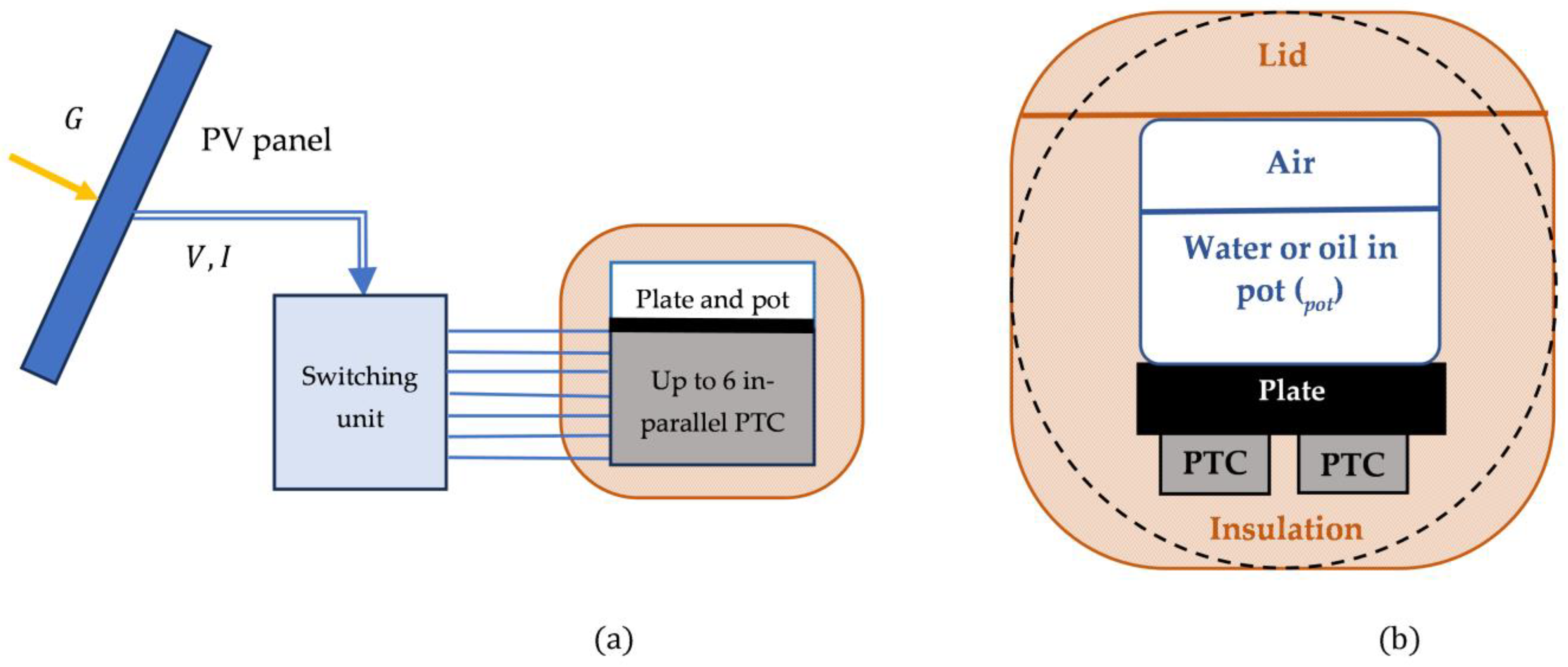
Indoor cooking. Direct and indirect solar cooking is based on heating the cooking pot or a heat transfer fluid by irradiance absorption and its immediate conversion into heat, Arunachala [15]. They offer relief for the above-mentioned problem. These thermal cookers must be operated outdoors, at least partially, with low social acceptance, in addition to risks of robbery, dust, and animal aggression. To allow indoor cooking, direct cookers concentrate the solar rays into a hole in a dwelling wall, e.g., the Scheffler parabola, or other options, e.g., Balachandran [16] and Singh [17], while indirect types use a heat transfer fluid to bring heat from outdoors to the cooking utensil, which can be located indoors, e.g., Varun [18]. Varun [19] reviews the topic with particular emphasis on indoor cooking, stating that it is the need of the hour. Sizable solar cookers produce steam to cook indoors using steam indirectly, typical for temples in India, Indora [20]. There is a need for practical layouts for family-size solar cookers allowing indoor cooking in a conventional kitchen. The quality of the food and the life quality of the housekeeper increases. To fulfill this need, Photo-Voltaic (PV) panels as a primary energy source seem suitable for this, since the panels can easily be affixed to the roof. This technology is supported by the continuous decrease in PV panel prices, which have reached the order of 0.1 €/nominal watt (peak) wholesale, IEA [21], and [22] by Our World in Data. Even today, there is no technology widely used for off-grid PV cooking of the family size, although some studies address its viability, such as Dufo-López [23], Altouni [24] and Batchelor et al. [25] among others.
The heating produced by dissipating the electricity of the panels into heat can also be applied to heating air for drying vegetables, meat, or seafood, which is not the aim of this article. Moreover, the proposed heaters can be added to a kind of commercial electric pressure cooker, Rose [26] modified it to accept PV electricity, but still, they are not available. These devices substantially reduce the thermal energy loss of water evaporation. Simultaneously they incorporate some thermal insulation, reducing sensible heat losses, Asok Rose [27], thus also increasing energy efficiency.
Solar panels and direct drive. PV panels are sets of in-series solarized reverse-biased diodes that offer a direct electrical Current (DC) approximately proportional to solar irradiance times exposed area. However, they show a non-linear dependence on voltage. Moreover, partial shading on a conventional panel causes a considerable loss in conversion efficiency, which in standard operating conditions is 17% to 24% for silicon-based cells. All this makes an electronic controller for establishing the appropriate operating voltage and the resulting intensity necessary. These controllers, on the one hand, try to maximize efficiency and, on the other hand, adapt voltage for electricity use, e.g., [24]. Usually, the controller is embedded into the so-called inverter, as these types of equipment aim to inject Alternate Current (AC) electricity into some kind of grid, either mains or micro(smart)-grid.
When this is not the case, the Direct Current (DC) produced by the panels is usually directly consumed, sparing the inverter, e.g., Simon Prabu [28], and Atmane [29] among others. There are commercial devices that rely on charging a local battery for later use while eventually supplying a load. Using these devices makes it necessary to transport the costly, heavy, and short-lived batteries at large distances, carrying the possibility of the users abandoning them in situ when dead, with the associated pollution of the environment. These controllers/chargers are designed for standard voltage panels, such as 12 V and 24 V, for the battery’s requirements. These voltages are not aimed for by the standard nowadays of massively produced panels but are in the range of 30 to 40 V for panels made with in-series 60 to 72 cells, or twice in the case of the split cell type. Matching the panel intensity and voltage with the battery charge and discharge requirements wastes substantial energy and limits the power to the additional connected load. I Zobaa [30] states that PV panel output to user electricity can be as low as 50% under normal operation. Moreover, these controller/charger devices incorporate integrated electronics and batteries that, in the event of a malfunction in a remote or isolated location can rarely be diagnosed and replaced, making them somehow undesirable, especially for low-income economies.
As a preliminary consideration, it is worth establishing if the silicon PV panels are efficient enough for family cooking. Assuming 20% as the representative efficiency from solar energy to electricity, it follows that this is lower than the representative efficiency of a thermal solar cooker, which is around 30% maximum, e.g., Onokwai [31]. This later low figure incorporates the need to reorient the thermal solar cooker to stay focused. This operation is seldom performed daily as frequently as needed and can be non-perfect. In the case of a PV-based electric cooker, sun tracking is possible but non-compulsory as there is no sun ray concentration. The electricity can be dissipated into useful heat in direct contact with the electrified cooking pot and is always internal to the thermal insulation. The peripheral thermal insulation results in reduced ambient losses, positioning electrical cooking in an advantageous position. A roof-mounted PV panel is usually in a fixed orientation towards the equator, thus losing some direct radiance, but it captures the diffuse component.
The paper focuses on this technology. Moreover, the low ambient losses allow an increase in cooking temperature, suitable for frying, braising, and the like. One inrush into this technology is Watkins [32], who cast the term Insulated Solar Electric Cooking (ISEC). The peak power of a single silicon PV panel in the market is between 300 and 500 W at the present state of the art, enough for this kind of cooking. If this is not enough, the proposed configuration allows for adding panels in parallel, thus ensuring a safe voltage and multiplying the intensity. This way, the increased power can be used in a single high-power hot plate or several ones, thus allowing recipes needing in-parallel cooking of several ingredients.
This work addresses the possibility of eliminating both electronics and batteries, in an independent installation of an apriorist single PV panel and a thermally insulated cooking pot. No other publication has been found on this layout nor has a model describing it. An approach is Osei [33]; there, nichrome heaters are embedded into erythritol Phase Change Material (PCM) used as thermal energy storage. The resistors are directly connected to a PV panel to form an integrated unit. When directly connecting conventional resistors to PV panels, there is a primary difficulty. As no electronics are present, it is difficult to efficiently dissipate electricity using the almost constant resistance such as nichrome wires for different irradiances. In the mentioned work, this problem is overcome: a string of diodes has been tried as heaters directly connected to a PV panel to better match the panel intensity-voltage I-V curves so that operation near the Maximum Power Point (MPP). Some thermal problems arise with the diode semiconductors’ thermal breakdown. The present paper illustrates these issues and, as a consequence, proposes using ceramic Positive Thermal Coefficient (PTC) commercial resistors as heaters, Wikipedia [34] and Yang [35].
There is an unavoidable thermal resistance from the PTC heaters up to the cooking pot. It can be avoided by using induction heating at the pot bottom, although this incorporates electronics. Some studies address the topic of designing such devices using the DC electricity available from a PV panel, e.g., Sibiya [36], Anusree [37], and Dhar [38]. Even a commercial unit with an inbuilt controller and a battery has been found, Greenwax Technology [39]. This attractive option finds an additional drawback; it needs special cook pots not always available in some communities.
In the analyzed simple layout that avoids a battery, there is no purpose for electrical storage for off-sunshine cooking, e.g., batteries. Complementary methods can overcome this. The recently cooked meal is hot, so it has in-built thermal storage, and having it warm later on is an extra value. When cooking, the yield produces a moderately elevated temperature in the food. This forms what is called Thermal Energy Storage (TES) to replace electricity storage. It is common to use “wonder bags”, Mawire [40]; this means storing the already-cooked hot meal inside a heat-insulating bag or box and even complementing this heat storage capacity with some extra material storing sensible or latent heat, Lecuona-Neumann [41]. This will not only keep the meal warm for later use, e.g., up to dinner time but also prolong low-temperature “slow cooking” without any extra energy consumption. Another possibility is to incorporate a Phase Change Material (PCM) as a TES with a higher energy content, 100 to 400 kJ/kg, than a single-phase material, although at a higher cost, e.g., Opoku [42]. Such materials can be paraffin, erythritol, mannitol, xylitol, and other non-organic ones, Santhi Rekha [43]. Storing the melted PCM in a well-heat-insulated vessel can maintain its temperature above solidification. The latent heat of solidification re-heats and even can softly cook breakfast from the previous day’s collected solar heat. Some of these materials are non-toxic or polluting and are mass-produced, Lecuona [44] and Agyenim [45] among others.
Not including storage in the initial layout does not preclude using the surplus electric PV production for charging appliances such as mobile phones, lanterns, radios, and the like, as needed for enhancing the quality of life in the home, as their consumption is typically lower than of a solar cooker.

2. Materials and Methods

The methodology chosen is based on a mathematical model of the PV solar cooker described, using direct connection to the PTCs through a switching unit. This model uses commercial curves of PV panels to explore their direct connection to PTC commercial heating elements. Just as an example, a sample of resistance curves has been experimentally determined. The direct connection layout is developed. The aim is to offer a simple enough model and information so that a design and later construction is possible with confidence in the performances and for diverse sizes and solar resources.
Simple cases are modeled, taking as an example a single-family single hot plate representative size. The results are explained and discussed and finally, some conclusions are offered, such that PV-based solar cookers can be constructed quickly and reasonably priced, avoiding using electronics and batteries.
If during cooking a power reduction is needed there are two kinds of options, firstly mechanical, such as disorienting the panel or separating the pot from the hot plate by an insulating sheet; secondly, electrical, such as adding or switching the PTC elements off away from the optimum number of them.
The theory presented here uses the least possible complexity to reduce the computing requirements for a design to a minimum, allowing the use of widely available spreadsheets and, in an extreme case, a scientific calculator. It proposes a solution of appropriate technology for sustainable development and a tool for fighting energy poverty and food insecurity. For the construction, a multimeter, in addition to simple tools, is just what is needed. A sensible experimental calibration can counteract the loss of accuracy because of the low modeling mathematical order.

3. Results

Section 3.1 models a generic PV panel or set of panels in a practical way using only catalog data and the basic properties of these devices. Section 3.2 models the PTC heaters in the same way. Section 3.3 offers the model results of matching both devices as a function of irradiance and temperatures. Section 3.4 maximizes heat production. Section 4 models two extreme cases in a time-marching way, incorporating a model of heat losses to ambient. Section 5 summarizes the results and offers a set of usable conclusions.

3.1. PV Panel Modeling

Detailed and highly accurate electrical modeling of PV cells is possible when numerous required physical parameters are known. Alternatively, acceptable accuracy can be reached using the basic parameters of the materials and their layout. This is possible through a multiparameter prediction or even the least square fitting to the overall characteristic curves of a whole panel such that the delivered intensity can be formulated as I G , T P , V , i n t e r n a l   p a r a m e t e r s , reaching a respectable accuracy. 〈 〉 indicates functional dependence, G is solar irradiance, T P is the panel temperature, and V is the output voltage. Unfortunately, such curve-fitting leads to a non-linear procedure that is complex in application. Semiempirical variants are available using just some parameters when all necessary ones are not given, such as in commercial panels, such as Rawat [46] and El Tayyan [47] among others. Within these approaches, one finds fitting empirical formulations based on physically reduced models. This is a practical approach that is preferred for simplicity, reducing the number of parameters by using I G , T P , V , e m p i r i c a l   p a r a m e t e r s .
The particular model used in this paper follows Equation (1). It discriminates two voltage ranges above and below a reference voltage V r   G , T P   :
  • For voltages below this empirical reference, V < V r G , T P   , the intensity I is assumed to be proportional to irradiance G using the peak nominal values I p e and G p e for normalization. Within this range, I V is almost constant, near the value at the short circuit. It has a low dependence with V decreasing as Equation (1) indicates by the effect of in-series resistance R s , following the simple one-diode model. When operating, the panel temperature T P is higher than ambient temperature, requiring a correction that usually is referred to as a standard T P = 25   .
  • Beyond the specific reference voltage V r and the corresponding I r , a continuous exponential decrease considers saturation down to the open circuit voltage V O C when I = 0 .
                                      V < V r I = I p e G G p e 1 + γ T p 25 V R s                     V V r V = I r K d exp K e V V r r    
The fitting of this model to the commercial data, usually given by purchasers, has been performed in two ways: Equation (2) (a) is a simpler one and (b) a more accurate alternative which includes an extra fitting parameter to the expression of V r G , T P , leading to different parameter values.
a :   V r = V r 0 β T P 25 b :   V r = V r 0 β T P 25 + V r b G b G 1 b ; G > 0
The extra correction to V r of option (b) allows reproducing V 0 C G   b e t t e r , especially for low values of G . These two alternatives allow for comparing two slightly different fitting options on the same panel data. Unfortunately, the adopted model does not give an explicit expression for the voltage at the Maximum Power Point (MPP) called V M P P , which happens at the point that maximizes W V M P P , G , T P = I × V V M P P , G , T P . This means max I × V   d I × V d V = 0 .
In what follows, the model is applied to an average-performance solar panel. It is representative of the average PV residential market. This one has a 1.85 m2 aperture area, delivering a nominal peak power of W p = 310   W . 
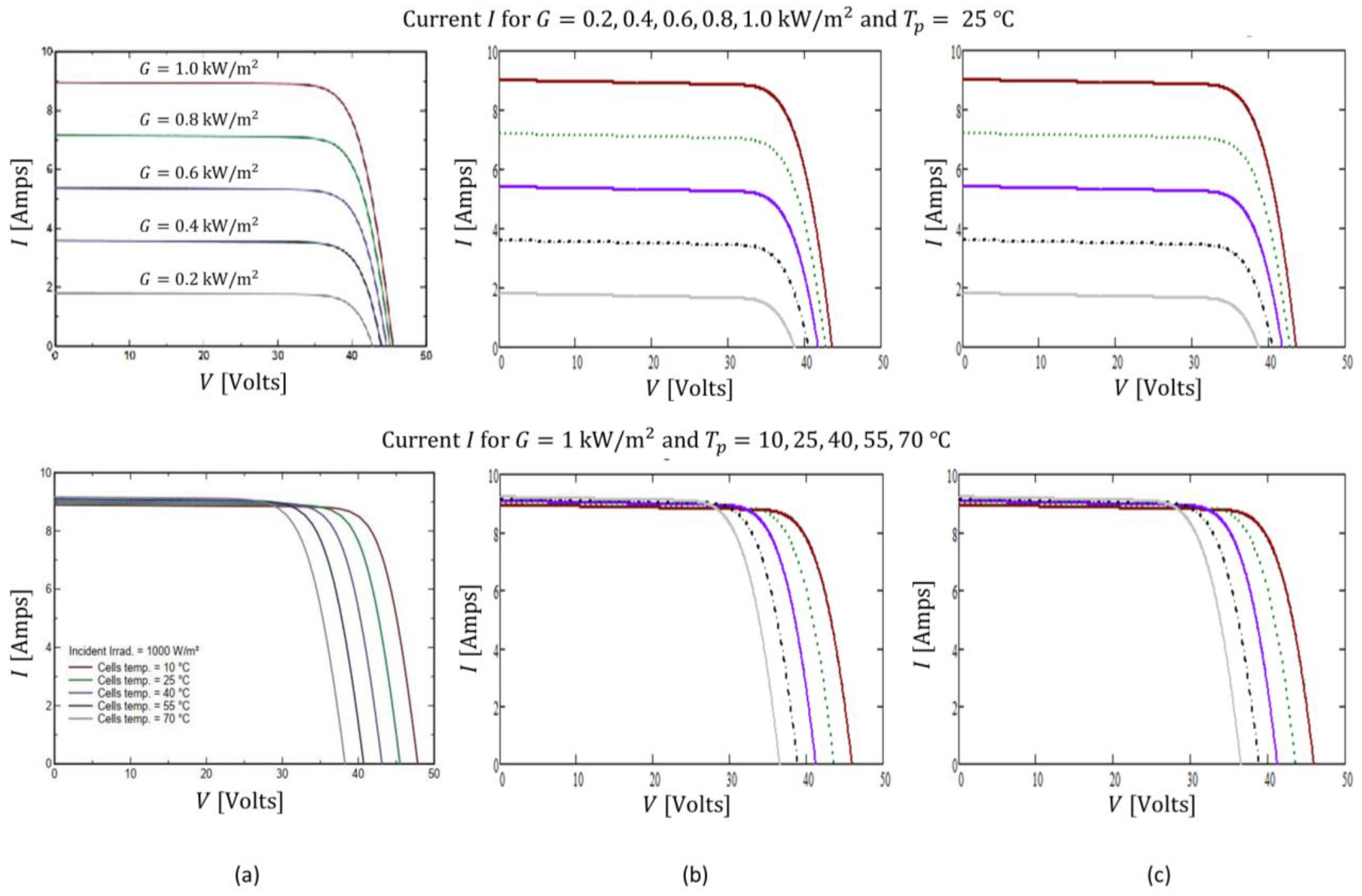
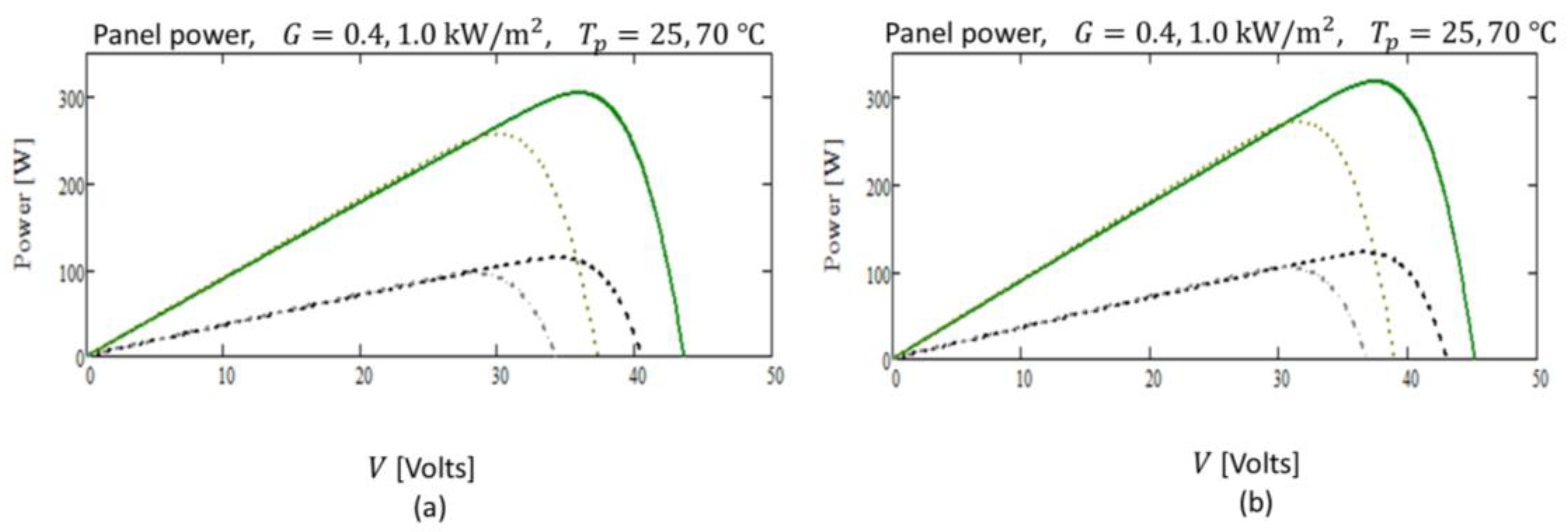
Figure 1 shows the results of fitting both options in Equation (2). Equation (3) shows the set of empirical and manually fitted parameters. The resulting maximum peak power values obtained are (a) W p e = 306   W and (b) 319 W. The most crucial zone in the I V map is the corner of the curves as the power reaches its Maximum Power Point (MPP) as max I × V d I d V = I V < 0 ; this condition can only happen there. Figure 2 shows the results.
Now it seems clear that a fixed resistance R = V I = c n t . , i.e., the inverse of the slope of a straight line passing from (0,0) in the V I graph, can only intercept a single MPP corresponding to a single G and T P . Figure 1 allows us to easily reason the problems associated with feeding a fixed resistance, R , with the PV panel. It would impose a fixed straight line of operation: I = V / R , coming from (0,0) to intercept the panel curve. If the value of R is chosen for the line to intercept the panel curve at the MPP for certain G and T P , any variation on one of these parameters shifts the MPP away from the intersection.
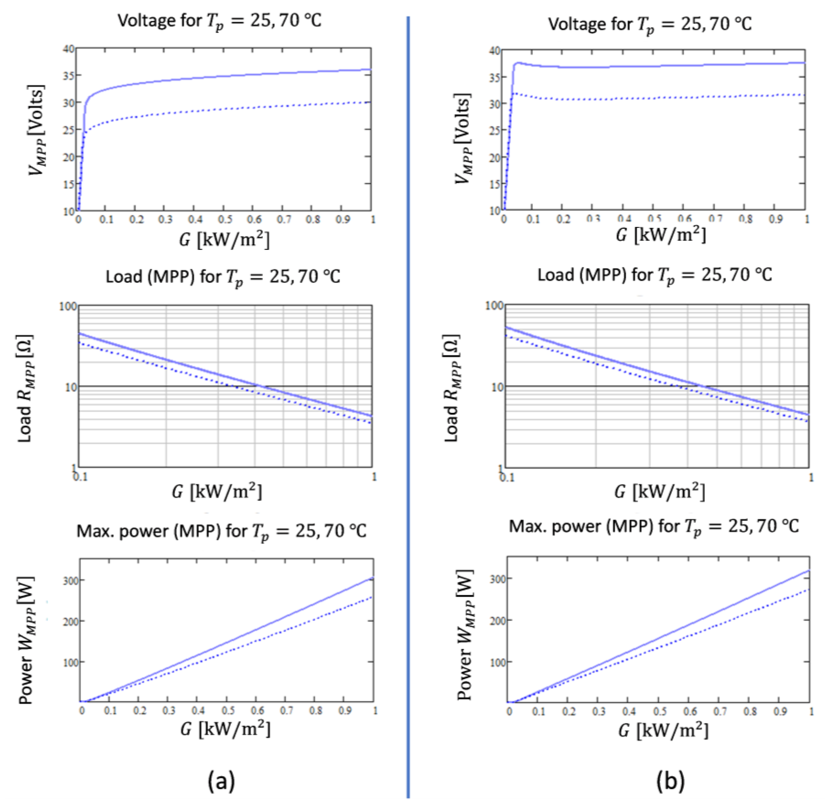
Figure 3 shows the required value of R for operation at the MPP for different irradiance values and working temperatures. Both optional fits defined in Equation (2) are displayed, evidencing slight differences. It shows that the MPP happens at a relatively constant V ,     G and the resistance for MPP decreases with G . It also shows the linearity of the maximum power achievable G .
I p e = 9   A ;   G p e = 1   k W   m 2 ;   γ = 5 × 10 4   A   1 ;   R s = 200   Ω V r 0 = 18   V ;   β = 0.16   V 1 ;   K d = 800   A ;   r = 1.5 ;   K e = 70   V ;   b : V r b = 1.5   V ;   b = 0.4
If a variable linear resistance R loads the panel working continuously on the MPP, it must increase for lower G , and it has to be sensitive to T P . This is evident from the fact that V M P P c n t . for fixed T P . Figure 2 shows the differences in power for the two optional fittings, especially on the MPP voltages, in the order of 10%.
The usual large variations in irradiance during panel operation and the associated need for a variable load resistance justify the need for a controller. It can be either the Pulse Width Modulation (PWM) type or the perturb-and-observe tracking type [48]. Both are commercial implementations. They require a microcontroller and a battery, plus power electronics. They are oriented to properly charge and discharge the battery. The ideal way out for MPP tracking (MPPT) would be a non-linear charge that would present every time the resistance maximizes the panel power W M P P , from now on R M P P , in an automated way. Figure 3 represents the voltage, the R M P P , and the resulting power for two values of T P . Observing it, the trends highlighted are evident. Some differences can be appreciated between both fits, but overall, they are equivalent. There is an almost linear change in W M P P with G .
Figure 3 also shows that for this panel V M P P is around 25 to 32 V at the representative temperatures resulting from a cloudless day with no wind, here simplified to T P = 70   . Incidentally, this is not too far for charging 24 V batteries. These calculations could be improved by using a time-varying T P , but this would oblige to describe a time marching of the operating point of the panel using the NOCT (Normal Operating Cell Temperature) parameter, Alonso [49]. It would also require information on the not-always-available day temperature and wind speed, which can be quite different from day to day and for distinct locations.
As a preliminary conclusion, avoiding electronics calls for a non-linear and/or variable load. In what follows, the selected case is Positive Thermal Coefficient (PTC) variable resistors for heating.

3.2. PTC Modeling

PTCs can be defined as thermally sensitive semiconductor resistors. They are polycrystalline ceramics based on barium titanate, Abidi [48], and Alonso [49]. They correspond to a class of materials named crystalline ferroelectric ceramics, which are obtained by sintering a powder typically of barium titanate at temperatures up to 1400 °C. PTC heating elements are a kind of thermistor, so they share the same principles of operation. During the fabrication of the PTC heaters of interest, dopants are added to give the material specific semiconductor properties.
With the PTC temperature rising above a reference ambient T a t = 25   , the resistance of the PTC initially decreases exponentially with a thermal coefficient α l o w = d L n R d T < 0 , behaving like an NTC. For a near ambient temperature (e.g., 50 °C), the resistance becomes relatively constant up to a second tailor-made temperature, (e.g., 100, 150, 200, 250 °C) where a phase change occurs. Above this temperature, the resistance rises steeply at a larger α h i g h = d L n ( R ) d T > 0 and > α l o w . 
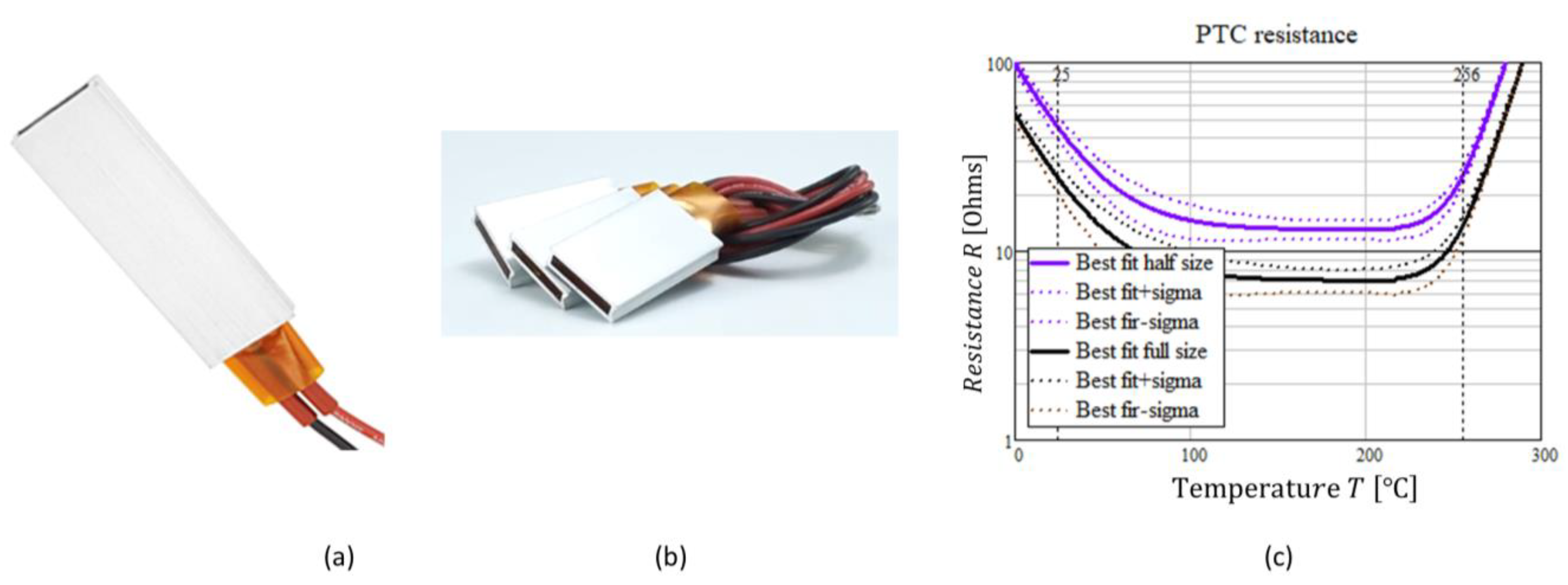
Figure 4 shows a realistic curve for resistance as a semi-logarithmic chart of a generic encapsulated PTC available from Asian suppliers of an active size of 60 × 21 mm, which from now on is called “full size”. It is recommended for a voltage range available in the PV panel presented above. This resistance corresponds to a non-loaded PTC at a very low voltage, such as the one applied by a DC multimeter. Loaded PTCs suffer from self-heating, changing in a non-negligible amount the apparent resistance R = V / I , especially at high dissipated power. The Steinhart–Hart equation is often used to approximate this rise, Wikipedia [50]. Other models are available. Beyond the range of the large resistance rise, the resistance again decreases out of our range of interest, and eventually, a breakdown occurs. The temperature where the resistance duplicates above the minimum is called the Curie temperature T C . It is considered a limiting temperature due to the sharp reversible cutoff of power it produces, implying a safety mechanism against overheating. PTC heating elements are used widely; fuel pre-heating, compartment air warming, air hairdressers, defrosters, silicone cement melting pistols, evaporators, boilers, and electric motor protection are just a few examples. Samples can be bought for around one € and one-tenth of this in quantities.
For a low applied voltage, the resulting low-temperature high resistance, and its decrease as the temperature increases together help approach the PV panel MPP at low irradiances, such as in the morning, Figure 3. Energizing the PTC at an initially cold state implies feeding a large resistance with the resulting low intensity. As the temperature increases, the reduction in resistance helps raise the PV panel curve towards the MPP. If the MPP passes a low PV voltage region, an excessive reduction in dissipated power would result in a reduction in temperature with a consequent backward displacement towards the MPP. From another point of view, the large resistance increase near the Curie temperature helps limit the temperature as a thermostat would do. T C 250   is selected for the present application to avoid burning the cooking pot or its thermal insulation. The resulting hot plate temperature allows meat frying and roasting in a pot or other utensil, Sagade [51], as well as food preservation, Berk [52].
Commercial PTC heating elements sold by generic suppliers show a slender flat tablet structure. They are circular or rectangular, of ≅5 mm thickness, with both sides metalized as electrodes. They usually are offered bare or electrically insulated by a temperature-resistant plastic socket. In the latter case, the set is pressed inside a flat aluminum tube, with two side leads for electrical connection insulated from the outside by a temperature-resistant material, as depicted in Figure 4. The generic commercial PTCs are specified by a few parameters: (i) the recommended supply voltage V s , in our case 36 V; (ii) the minimum resistance temperature T m ; (iii) T C , or an intermediate one. Eventually, some nominal or maximum acceptable parameters are available, such as (iv) the recommended power W o p although this is rarely specified; (v) the maximum continuous temperature; (vi) the maximum or breakdown voltage. With PTCs being a distributed resistor, as the electrode area increases, the usable power is proportional to it, and the resistance is inversely proportional, ceteris paribus. The unloaded resistance vs. temperature can be measured by heating the PTC and when offline immediately measuring R , Boubour [53]. Thermally insulating the PTC allows for surpassing T C . An operating resistance can be obtained as R o p = V o p 2 W . This method does not give exactly the same result, presumably because of self-heating, Musat [54].
In our case, after a measuring campaign using laboratory-grade instrumentation for measuring resistance, voltage, and DC intensity, R T has been obtained. These curves were obtained using a stabilized power supply to reach the indicated temperature, which was measured by a calibrated K-type thermocouple located inside the PTC. The temperature was stabilized by two massive aluminum blocks reaching a steady state for half an hour. The differences in the PTC resistances resulted in the expanded ±(2σ) interval around the average. Figure 4 shows the ± σ interval to avoid overlapping. This was much larger than the Gaussian combined uncertainty of the thermocouple of ±1 °C and of the multimeter and power supply of 3 1/2 digits of accuracy. The number of PTCs tested was twenty and a normal distribution of resistance was checked. Equation (4) shows the data fitting expression proposed for the PTC resistances used for loading the PV panel. The rationale of the proposed expression is that the thermal coefficients α apply smoothly around the minimum resistance R m R 0 through the combining exponent n .
    T < 0.87   T C R = R 0 1 + exp α l o w T 0.19 T C n 1 / n   othervise R = R 0 1 + exp α h i g h T T C n 1 / n
Equation (5) indicates the appropriate values found for several samples tested of generic encapsulated PTCs with an active size of 35 × 21 mm and a recommended supply voltage of 30 V given at R 0 and a maximum power of 162 W. This size is called “half size”. When applying the fitting function, the minimum resistance resulted in R m = 7.03 ± 1.0   Ω , R 25 = 25 ± 5.0   Ω , and the fitted T C = 256 ± 6   with R T C = 15 ± 1.0   Ω , and 0.19   T C 1 is an empirical value. Figure 4 shows the resulting continuous function and the experimental variation found.
T C = 250   ; R 0 = 7   Ω ;   n = 1.5 ;   α l o w = 0.04   α h i g h = 0.067  
Neither the applied power nor the load resistance of a single PTC element can be suitable for all the range of G and T ; the number P 1 , S 1 of, respectively, in-parallel connection of P sets and of in-series strings of S elements are considered to load the PV panel. This way, the total resistance becomes R Z ; Z = P S . P = 2 ,   S = 1 Z = 2 and is anticipated as suitable in our case, but at the limit for dissipating the PV panel rated power at a PTC temperature corresponding to R 0 . The following section illustrates this point.

3.3. Direct Matching of the PV Panel with the PTC Heater

This section calculates the useful power that results when connecting both the selected PTCs and the PV panel, specifying T P but leaving G and T free. When compared with the power at the MPP at each T P and G condition, one can figure out how far from the optimum the operating point is. 
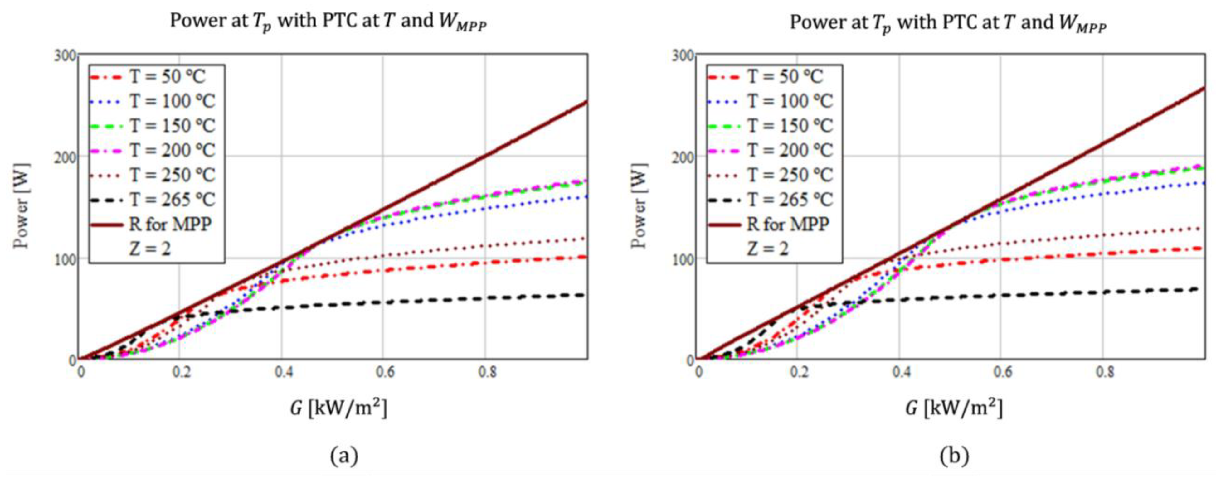
Figure 5 shows the results for the (a) and (b) fits for Z = 2 with half-size PTC heaters. Differences between both panel fits are negligible, as the knee of the curves is only marginally affected. For the two in-parallel identical half-size PTCs selected in this case, and for low G , the power is close to the MPP for a wide range of T but separates progressively for G 600   W m 2 , suggesting that a lower resistance would be more suitable.
This Z = 2 connection also suffers from another limitation. The recommended maximum power through each single PTC of W 1 l i m i t = 65   W is surpassed when @ T < 265   and G 150   W m 2 . The excessive power will be limited for T 265   but separated progressively from MPP as G increases. Even duplicating W 1 l i m i t , the Z = 2 connection restricts the near optimum power for low G s, as Figure 5 shows.
A more progressive stair of higher to lower resistance range would have six of the widely available half-size of the selected PTCs for an in-parallel layout and three switches. The possible single connections positions are as follows:
  • Position 1: Switch 1 ON and the others OFF, one PTC connected ( P = 1 , S = 1   Z = 1 ), highest resistance.
  • Position 2: Switch 2 ON and the others OFF, two in-parallel PTCs are connected ( P = 1 + 1 = 2 ,   S = 1 Z = 2 ).
  • Position 3: Switch 3 ON and the others OFF, three in-parallel PTCs are connected ( P = 3 ,   S = 1   Z = 3 ).
This way, combining the three ON/OF in-parallel switches makes six different equally stepped combinations of half-size PTCs: Position 1, one PTC active. Position 2, two PTCs active or a single full-size one. Position 1 + Position 2 activates three PTCs so that Z = 1 + 2 = 3 , equivalent to Position 3 alone. Position 3 + Position 1, Z = 4 . Position 2 + Position 3, resulting in five active PTCs, Z = 5 . Position 1 + 2 + 3, all switches ON, 1 + 2 + 3 = 6 in parallel resistances, Z = 6 . No in-series resistances have been contemplated in the present design as the voltage of a single PV panel is acceptable for the PTCs considered. Several in-series PV panels to multiply power could be contemplated but using a higher unsafe voltage. In parallel, equal PV panels would require less load resistance, thus a high Z , not only to match them but to avoid PTC overload.
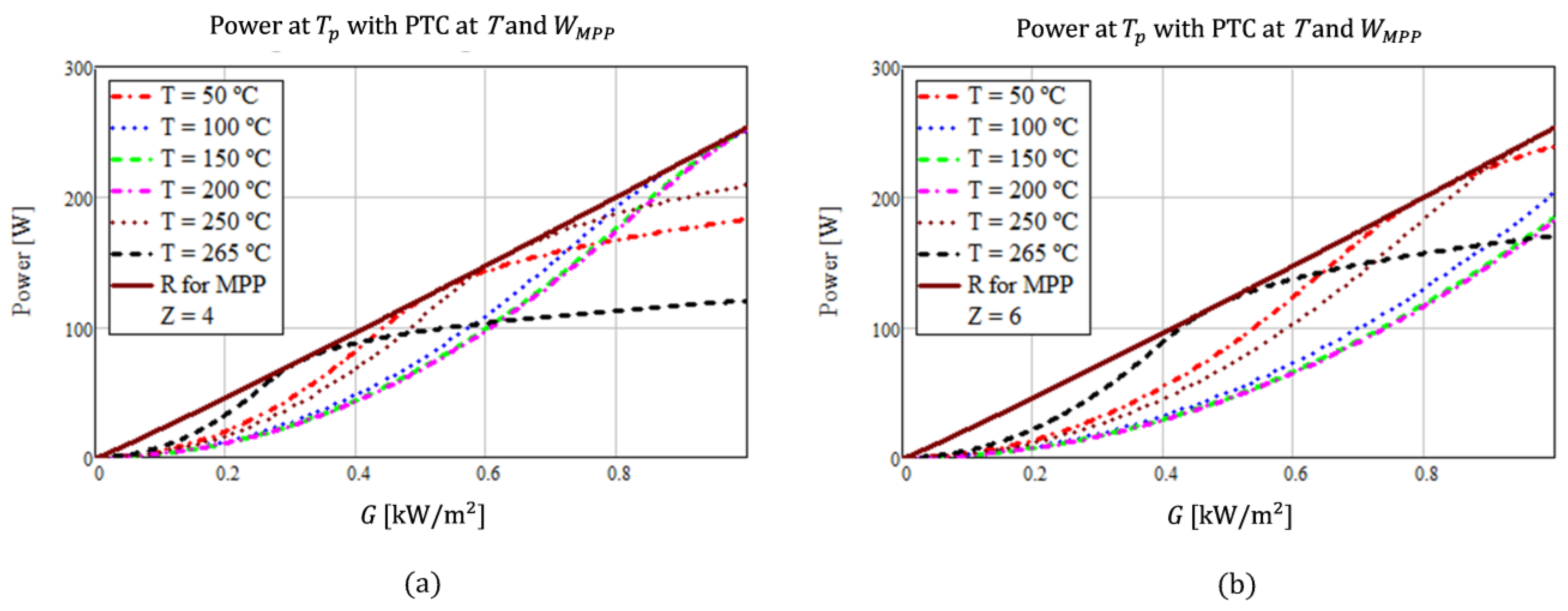
As a comparison with Figure 5, Figure 6 shows two cases with more resistance. Both Z = 4 and Z = 6 can be near MPP for large values of G , but they separate for low values of G , indicating that a low value of Z is necessary for low values of G for approaching MPP, indicated in Figure 5. For Z = 4 , W 1 , m a x = 65   W and for Z = 6   W 1 , m a x = 32   W , both happening at G p e = 1   k W m 2 and for T < T C . Both figures corroborate the suitability of the connection scheme using the 3 switches indicated above. Curiously, K = 6 ,     T = 50   is near MPP @ G p e = 1   k   W m 2 but unless a cold object is in good thermal connection with the PTCs, heating will occur immediately, making this equilibrium solution not realistic. This calls for a time-marching analysis.
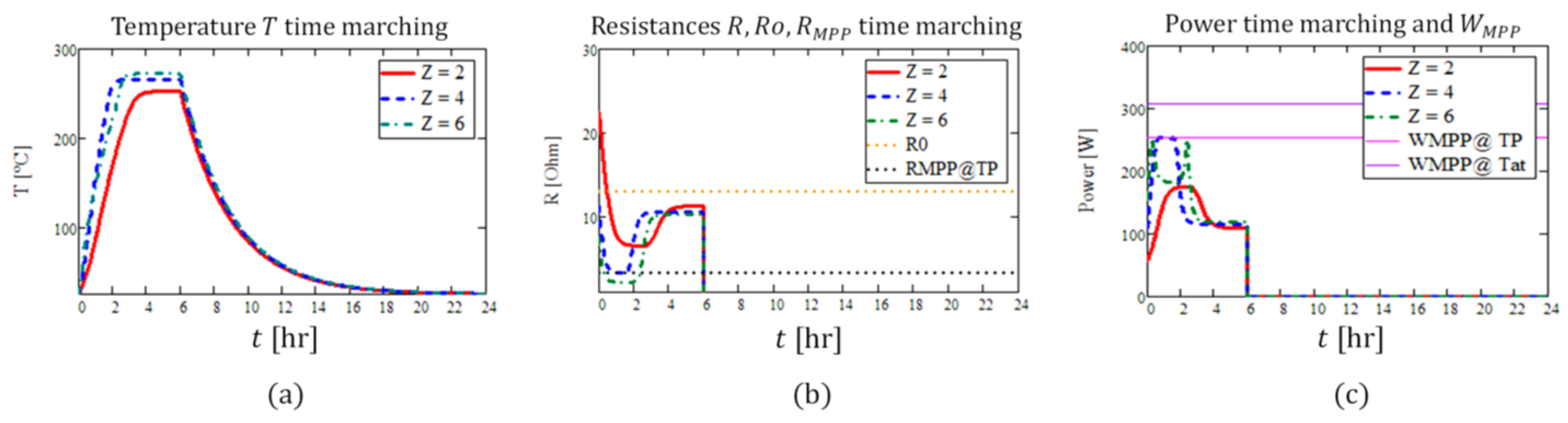
The PTC temperatures can temporarily be different among them, e.g., during heating when some of them are recently connected and have a lower temperature than the others located side by side that have been operating for a longer time, i.e., with self-heating. In a short time, PTC temperature homogeneity is reached owing to the low heat capacity of the PTCs.
This exercise clears the intervening non-directly-controllable factors, G and T , besides T P . There is some way for the operator (or the controller) to select T , the PTC temperatures, by switching a number of them depending on the pot’s temperature. Two examples are offered in Section 4 to illustrate these issues.

3.4. Practical Maximization of Power

As PTC resistances can only be modified by their temperature, the remaining possibility is to switch a combination of PTCs to approach the MPP as much as possible, as analyzed in the previous section. This can be performed by a continuously operating perturb and observe technique. An automatic version would switch resistances through CMOS electronic elements, [53], preferably in the correct direction toward MPP, using a programmable microcontroller, and stay if there is an increase in W . This requires electronics.
A straightforward alternative technique is to offer the user both a Wattmeter (electronic), which nowadays can be purchased at a moderate cost (around 4 €), and manual switches so that the operator decides. After a learning period, the correct manual selection can be anticipated. In the specific layout selected here, the following exercises corroborate that only large resistances seem advantageous for the lower irradiances G to approach the necessarily low maximum power. An additional consideration is that low G s means low W so approaching the MPP is of less importance than for high G s.

4. Time-Marching Modeling of the Solar Cooker

4.1. Preliminaries

For heating a non-flowing bulk thermal capacity C   [ J K 1 ] , the steady-state temperature has been modeled by Wang [55] in a simplified layout similar to the one in this work, obtaining a dimensionless correlation for the dimensionless overtemperature θ = T T a t . Here, the model is refined by including the transient stage. A single lumped parameters 0D heat balance model of the entire system is used for our purpose, Equation (6). No ohmic losses are considered between the panel and the PTCs.
C d T d t = C P T C + C p + C p o t d T d t = I V W U A T T a t
U A is the heat loss conductance through a control surface A in the heat path toward the atmosphere, with an overall heat transfer coefficient from the system to ambient U . This equation allows determining the shared system temperature T . Again, both I and V are such that W = W T , T P , G . The stagnant (steady-state) temperature T s is determined by W T s s , T P , G = U A T s s T a t   where U would depend on T and other operating parameters, such as external wind and T a t .
This model is similar to the one proposed by Musat [54]. For this equation to be accurate, the Biot number B i of the thermal mass of the system must be low enough, Incropera [56], Equation (7). Considering an axisymmetric internal layout, the radial temperature gradient is considered negligible in front of the axial one. Figure 7 depicts the general layout of the connections and the cylindrical layout for the prototype. It consists of the PTCs below the flat heated plate of diameter D p and the closed pressurized pot above it of average diameter D p and height H p o t = 0.07   m . The overall height of the PTCs, plate, pot, top and bottom insulation, considering sphericity, is H D p = 0.14   m . Let us consider the in-series elements in the 1D geometry: from the PTC, plastic socket (S) + aluminum wall (a), to the flat hot plate (p), from the plate to the pot’s inner bottom (pot), and from it to the liquid inside the pot (f). The external cylindrical closed surface can be the result of a tight insulation wrapping A i n = π 4 D p + 2 δ i n 2 + π D p + 2 δ i n H is of a similar extent to a spherical one A i n = π D p + 2 δ i n 2 . The relation between the Biot number and the effective heat conductivity k from PTCs to water is Equation (7).
B i = U A k H P T C w A p ; H P T C w = H S 0.1   m m + H a 1.2   m m +   H p 6   m m + H p o t 1.5   m m + H f D p / 2 = 79   m m δ i n = 20   mm ;   A A p = π D p + 2 δ i n 2 π D p 2 4 = 6.6
This leads to Equation (8), expressing the compound’s effective internal heat path length of the set H H and the effective axial heat conductivity k :
k P T C w H P T C w 1 = k S H S 1 + k a H a 1 + K P C T / p 1 A P T C A p + k p H p 1 + K p / p o t 1 + k p o t H p o t 1 + h f 1
According to Incropera [56] and Thermopedia [57], the contact thermal conductance K between flat surfaces under low joining pressure (screws for each PTC) can be estimated as K P T C / p 1.4 × 10 4 W m 2   K . For the plate/pot estimate, a realistic value can be orders of magnitude lower than the PCT/plate value because of the lower joining pressure (gravity) and the more extensive area of contact between the plate and the pot’s “flat” surfaces. This is in addition to the larger thermal distortions of flatness plus the typical high roughness of pot bottoms. K p / p o t 1.4 × 10 3 W m 2   K is assumed, as a conservative value, taking into consideration that a pure conductive air layer of 0.1 mm thickness would give K p / p o t = 320 W m 2   K . The result is, considering equal transfer areas K P C T / p 1 + K p / p o t 1 = 0.79 × 10 3 m 2   K W . The conductivities of the materials of the plates are, for Kapton® PTC socket, k S = 0.20 W m K ; aluminum cover k a = 240   W m K ; brass hot plate k p = 150   W m K ; steel pot wall k p o t = 35   W m K . One can estimate, according to [56], for non-boiling oil or water, a heat transfer coefficient from the pot bottom to the liquid bulk h f = 50   to   1000 W m 2 K . We can adopt an average value of h f = 500 W m 2 K . All this results from Equation (8) in k P T C w = 14.5 W m K . This small number suggests instead of a single temperature model, a more complex one is made from two or three bulk thermal masses. Section “Three Bulk Thermal Masses” analyzes this issue.
A value for U can be estimated as an in-series of (i) atmospheric heat transfer and (ii) thermal insulation of a non-technical (discarded tissues, hay, dry leaves, …) insulating material of an effective conductivity k i n 0.2 W m K ; this is larger than usual because of the relatively tight wrapping, the non-continuous covering and no external impervious cover. Taking into account a spherical external geometry, Figure 7 also accepts moderate wind convection and radiation to the environment, this sums up a heat transfer coefficient h o u t s i d e 12   W m 2 K , according to Rahmadi [58]. The radial conductance of the sphere shell is A i n U i n = 2 π k i n D p 1 D p + 2 δ i n 1 . Summing up, the result is U A = A i n U i n 1 + h o u t s i d e 1   1 0.48   W K 1 , the insulation effect (in) dominating this amount. This figure has been determined as realistic, although in the upper range, according to our own experimental results. All this ends up in B i 0.09 applying Equation (7). This value is low enough to expect a fairly homogeneous internal spatial 1D temperature, as B i 0.1 is the practical limit for accepting thermal homogeneity [56]. Precise thermal homogeneity happens after relaxation time τ h , following the stop of heat generation, i.e., the cooling process. From the 1D heat diffusion equation by conduction for our design with D p H , considering that C p o t C P C T + C p such that d T p o t d T = 0 during this period, Equation (9) yields its order of magnitude.
τ h = C P C T + C p + C w H P T C w k P T C w ~ 9.7 m i n
This τ h is much smaller than the free cooling time τ c o o with W = 0 , Equation (11), allowing full thermal homogeneity during the cooling process as a good approximation.
The Biot number reasoning is strictly valid for no internal heat generation, and we have heat generation on the lower border. Following this consideration, to estimate the maximum internal temperature difference Δ T s s , m a x , adiabatic 1D heat flow from the PTCs is considered at half the maximum panel power owing to the sinusoidal power profiles in Figure 8 and in the following ones This leads to Equation (10), which assumes the maximum panel power is accepting equal heat losses to electric input under steady-state operation (ss). Using m, kg, K, and s as units, the result is Equation (10).
Δ T s s , m a x ~ W m a x 2 H P T C w A p k P T C w = 22 K
If boiling water is in the open air, it happens at ≅100 °C; then, T C seems not to happen considering the roughly estimated thermal parameters. The maximum power will be reached with the appropriate resistors, according to Figure 4, as the low resistance PTC plateau will be reached even in this case. When heating oil or water up to pressurized boiling, according to Figure 4, the PTCs will also reach the low resistance plateau and even can reach T C so that heating can proceed with high power up to the limiting T C when power will stagnate.
To obtain preliminary information on the possibilities of the cooker as a function of the solar irradiance, the numerical resolution of a time marching equation, Equation (6), seems necessary. One must keep in mind that it deals with an average temperature. It gives quick information on the possibilities of the cooker, leaving for more complex models the discrimination between the temperatures of the different elements, e.g., a three-lumped-heat-capacities model, PTCs, hot plate, and pot, Section 4.2.1. Here, with a single lumped heat capacity, the rise in the temperature of the PTCs seems to be underestimated by an amount in the order of the result of Equation (10).

4.2. 0D Time Marching Results

Two reference scenarios are relevant: heating with (i) Constant irradiance, and (ii) cloudless day irradiance pattern. For simplicity, both use the PV panel curve fit with constant T a t and T P = 70   . Cooling with G = 0 follows. For both cases, Equation (6) has been numerically integrated using an explicit Euler scheme. Data at time step i allow obtaining T i + 1 , as d T d t T i + 1 T i Δ t , with some loss of accuracy but facilitating the use of spreadsheets. Solar time starting at sunrise is used in the cases solved. The resistance maximizing W has been calculated and is named R M P P .
The cooking medium has been represented by 1.08 L of pressurized water so that no boiling is allowed. Alternatively, we use glycerin weighing m = 1.7   k g of average specific heat c = 2.67 k J k g K equaling the heat capacity of water. This is for mimicking frying. With Equation (6) one can check that the characteristic cooling time when T T a t T m á x T a t = exp ( 1 ) can be obtained by setting I = 0 and constant parameters:
τ c o o ~ C P T C + C p + C p o t C U A = 3.0 h τ h
In practice, C = i m i c i is easily determined, but not U A . During a cooling experiment, measuring the temperature time marching results in a series, having T i at each time t i , U A i can be determined on the grounds of Equation (6), resulting in Equation (12). The resulting series can be improved by an eventual moving average smoothing to remove noise, Lecuona-Neumann [41].
U A i = m c i T i T a t , i T i + 1 T i 1 t i + 1 t i 1
These values of U A i can be used for further studies. Here, the datum already theoretically calculated has been used as it is coherent with its own experimental values.
  • For constant maximum radiance. The constant G p e for several hours can be attempted if tracking the sun. It would be representative of starting 3 h before noon and using the solar power up to 3 h in the afternoon, even without tracking. As a general case, after reaching the maximum temperature, stopping power reveals the free cooling process after t e n d = 6   h . Figure 7 gives slow cooking ( T > 70   ) for 5 h after t e n d and warm food for almost 10 h after, ensuring a warm dinner. Halving U A , e.g., duplicating the insulation thickness, approximately duplicates these times, ensuring warm food for breakfast the next day.
Figure 8 shows the results for three representative cases Z = 2 ,   4 ,   and   6 . The maximum temperature is achieved after t 2.5 h, with Z = 6 the highest, 272 °C. Reduction in power follows from surpassing T C in all three Z s. For all the cases, starting at 9:00 a.m. solar time, after 7 h, around 9 + 6 = 3 p.m., the temperature is high enough for cooking.
Power reductions after some hours of heating, Figure 8b, indicates that PTCs have reached the maximum temperature, beyond T C , and there is extra power available if the cooking process is required to heat food by immersion and/or evaporating water. In that case, the food would reduce the maximum temperature found for the PTCs, automatically increasing W . The individual PTC maximum recommended power of W 1 m a x = 65   W is surpassed for Z = 2 but not for Z = 4 and 6. The solar efficiency, Equation (13), for the invariable three Z s reaches η s o l a r 7 % . In the case of MPPT, it would rise up to η s o l a r , m a x = 13 % . If there is a wise selection of the available PTCs, an intermediate case would be the result.
η s o l a r = 0 t e n f W d t G p e × A P η s o l a r , m a x = W m a x G p e × A P
In Figure 8, the low PTC temperature from hours 0 to 2 h helps to deliver heat. However, this is uncertain because the single bulk temperature model adopted is limited. In reality, the PTCs under G p e self-heats in a short characteristic time τ P T C . Neglecting heat conduction and losses to the environment, as C p o t C p C P T C , the heating characteristic times differ, following Equation (14), where half the power and half the temperature increase are considered.
W ¯ W m á x 2 ; Δ T ¯ θ C 2 ; τ P T C ~ C P T C Δ T ¯ W ¯ = 54 s ;   τ P T C + p ~ C P T C + C p Δ T ¯ W ¯ = 4.5 min τ P T C + p + p o t ~ C P T C + C p + C p o t Δ T ¯ W ¯ = 1.3 h
As a result of these considerations, the PTCs could be in the low resistance plateau, near T C and correspondingly near R M P P after ≅1 min. After about 12 min, both the PTC and the hot plate can be near T C , while the pot is at almost T a t . Only after about 2.2 h, the full system can be near T C . Thus, the initial high resistance R indicated in Figure 8b seems not to happen unless the conductivities from the PTCs to the hot plate and pot are very high, and this does not seem to be the case for the high value of τ h , Equation (9).
A higher-order modeling will help differentiate the PTC/p joint heating. Only by discerning the three temperatures, PTCs, plate, and pot, can this issue be described in detail. The short time effect can be an increase in power owing to the PTC reaching the low resistance plateau or can be limiting after reaching T C . Figure 9 shows the extreme case when the pot contains a larger heat capacity, ten times the one already calculated. Correspondingly, U A is estimated as three times larger owing to the larger size, although its influence in the case analyzed is small. The model allows us to accept that the same result would be obtained while keeping all the previous data but with G = G p e / 10 = 100   W m 2 , typical of an overcast day. Only for Z = 6 is the boiling temperature reached after 6 h, just when power ceases. The total resistance for both Z = 4 and Z = 6 are near R M P P , corroborated by the power time marching near W M P P = W m a x . Both reach η s o l a r 10 % , which is near the maximum, Equation (13).
  • A cloudless summer day. A sinusoidal time distribution approaches the irradiance falling on the aperture area of a PV panel, even without solar tracking aimed to the equator with a tilt near the maximum solar elevation at solar noon. At the solstice its last t d = 14 h and reaches G p e , Equation (15).
G t = G p e sin π t t d t t d 0   f o r   t > t d G t t t d = G p e π t t d
This gives a characteristic heating time of several hours, alleviating the possibility of temperature internal differences that have been addressed in the previous paragraph.
If one imposes a fixed PTC temperature of the low resistance plateau, Figure 4, the power can approach W m a x t , as Figure 10 indicates with Z = 6 , with some fault near sunrise and sunset. If the PTC temperature follows Equation (6), the results are depicted in Figure 11.
One can notice that the higher resistance for Z = 2 fits very well R M P P for the first 2 h but fails to give power at elevated G s after 6 h; also, individual PTCs are overloaded. With Z = 4 , after 5 h T C is reached, limiting power. The case Z = 6 follows about 1 h later and reaches a higher temperature, Figure 11.
The power time marching, Figure 11b shows that starting with Z = 2 , switching to Z = 4 at t = 4   h after sunshine and switching to Z = 6 at t = 6   h approaches W m a x t = W M P P quite well up to the power limitation after t = 7   h .
The maximum heat available from the panel, with R M P P and no thermal losses can be the reference for the energy efficiency η d of the solar cooker alone, thus not including the efficiency of the PV panel, Equation (16). The results are 0.62, 0.62, and 0.59 for, respectively, Z = 2 ,   4 , and 6 , calculated with data from Figure 11. If the entire sinusoidal profile is reduced to 50%, power limiting is not reached as T t < T C . The efficiencies change to η d = 0.91, 0.51, and 0.37, respectively, highlighting the convenience of large resistances for low G s, e.g., Z = 2 .
η d = 0 t d W d t 0 t d W M P P , T P d t T P

4.2.1. Three Bulk Thermal Masses

The results and especially values for η d are a first estimation as the resistance increase in the PTCs at ambient temperature, already approaching R M P P , could not be accurate. This is a limitation of the single thermal inertia model that equals all the temperatures. Equation (17) indicates a three thermal inertia model: PTC, hot plate, and pot with its content.
a :   C P T C d T P T C d t = I V + K P T C / p A p T p T P T C U A P T C T P T C T a t b :   C p d T p d t = K P T C / p A p T P T C T p + K p / p o t A p T p o t T p U A p T p T a t c :   C p o t d T p o t d t = K p / p o t A p T p T p o t U A p o t T p o t T a t A = A P T C + A p o t
The PTC and hot plate lateral areas are considered negligible in front of the lateral, bottom, and top respective areas of the PTC and pot, Figure 7. U is common to the PTC, plate and pot.
It can be noted that, for the particular case of T P T C = T p = T p o t , the summation of (a) to (c) equations in Equation (17) gives Equation (6) with C = C P T C + C p + C p o t .
The previous section indicated that Equation (6) was not appropriate for early times. Here, a further insight into the early times seems to be illustrated. It can be considered that C p o t C p C P T C . Also, on the grounds of K P T C / p K p / p o t one can assume for the initial times that T P T C = T p ;   T p o t = T a t . Accepting the definitions of Equation (18), summation of Equation (17) (a) and (b) results in Equation (19), considering Equation (15).
θ T P T C T a t ; τ K C P T C + C p C P T C p A p K p / p o t + U A P T C + p C p A p K p / p o t
d θ d t + θ τ K = I V C P T C + p w t
This last equation assumes a linear power increase to approach the initial stages of Equation (15). As a result, this equation has an analytic solution given by Equation (20) in non-dimensional terms, assuming as initial condition t = 0 θ = 0 :
θ w τ K 2 = t τ K 1 + exp t τ K
This solution indicates a temperature linear increase versus the non-dimensional time t / τ K plus an exponential heat loss, negligible for t / τ K 1 , with τ K being the characteristic time, thus θ θ K . Equation (21) gives the values for τ K and w , according to Equation (18) and assuming MPP invoking the correct PTC resistance in the initial times.
τ K c P T C m P T C + c p m p A p K p / p o t = 16 s w = W m a x π t d C P T C + p = 253 W × 3.1416 14 × 3600 s × 353 J K 1 = 4.5 × 10 5 K s 2
This makes Equation (22).
θ K = w τ K t = π W m a x A p K p / p o t t t d  
Equations (20) and (22) with data from Equation (21) predict a quite slow and low temperature increase, thus removing the worry of initial times elevated temperatures, owing to the large conductance towards the pot here assumed and its very large heat capacity. If this conductance is ignored, an adiabatic evolution occurs, e.g., an unloaded cooker. Then, the reduced differential equation and its solution is Equation (23), which includes the value of w in Equation (21). It shows a larger overtemperature versus time. This indicates the importance of the heat transport to the pot.
d θ d t = w t t = 0 θ = 0 θ = W m a x C P T C + p π 2 t 2 t d
On the other hand, if one assumes constant maximum power W m a x , the solution of the full differential 0D equation for the subsystem PTC + p, Equation (6), with T a t = c n t . and t = 0 θ = 0 , results in Equation (24), but with only C P T C + p for the initial times considered. At these initial times, where the loaded cooker has the pot near ambient temperature while the PCTs and hot plate are rapidly heating, their thermal losses conductance to the atmosphere is meager, U A P T C + p U A , being one-half to one-third an upper estimation, according to Figure 7. Thus, the full solution, Equation (24), can be approached by the initial evolution, giving Equation (25), valid for t τ 1 although τ is uncertain because the uncertainty in U A P T C + p .
θ P T C + p , m a x = W m a x U A P T C + p 1 exp t τ   ;   τ = C P T C + p U A P T C + p
If one estimates U A P T C + p = U A / 3 τ = 37   m i n making the initial approach justified.
θ P T C + p , m a x t τ 1 W m a x U A P T C + p t τ = W m a x C P T C + p t
Comparing Equation (25) with Equation (23), a PTC+p subsystem heating occurs faster with constant maximum power than with the sinusoidal time profile. Equation (25) gives the initial time marching of θ P T C + p , m a x .
These solutions fail when the heat losses to the atmosphere are comparable to thermal inertia in terms of power, which occurs at time τ , or when the pot heating power becomes comparable to thermal inertia power, which is estimated in Equation (14), which becomes sooner. To analyze this issue and the resulting PTC + p temperature discrepancy with the pot, the full three thermal masses model needs further study.
As a conclusion, only with constant power from the beginning, comparable with the maximum power quantity, can the initial overtemperature of the subsystem PTC+p separate substantially from the pot temperature.

5. Conclusions

The proposed PV solar cooker allows indoor off-grid e-cooking and avoids electronics by directly connecting the right amount of PTC heaters to a solar panel or a plurality. No controller or battery charger is needed for its functioning, and it can reach high efficiency. The innovative design offers a better energy transfer from the PV panel to the cooker than linear resistors, reaching an electrical energy efficiency of up to 91% for a particular operation, even without any PTC switching. PTCs offer resistance growth at their low temperatures and a temperature-limiting effect, avoiding overheating.
The proposal is based on simplified models that have been developed to ascertain the adequate PV panel and PTC characteristics for this duty, illustrating the basic working and relevant parameters. The energy and temperature–time evolution has been described by a transient 0D ordinary differential equation that allows the use of ordinary calculation methods such as spreadsheets, thus allowing the dimensioning of a system with a small budget. The differential equation has been numerically solved using two representative forcing functions: constant peak irradiance for midday operation and sinusoidal irradiance mimicking a full-day operation. Both cases reveal relevant characteristics. More complex three bulk thermal masses have been analyzed to highlight some features without having to solve the whole mathematical model. Experimental campaigns will add valuable data to tune the models proposed for each implementation performed.
The model shows that thermally insulating the outside of the cooker is of paramount importance, which, in this case, can be performed with ordinary materials.
Switching several ordinary PTCs by any means offers the possibility of a wider energy match between the panel and the PTCs. The selected generic PTC heaters offer a good enough match for both low and elevated temperatures. Insufficient PTC resistance when starting cold with low irradiance can be overcome by disconnecting in-parallel PTCs and/or preheating either the empty pot or loaded with a small amount of oil for pre-cooking/frying or sauteing, as many recipes ask for.
Overcoming cloudy periods, extending cooking in the afternoon, and even cooking or heating breakfast before the next day’s sunrise is possible by heating a load of sensible Thermal Energy Storage (TES) or solid/liquid Phase Change Material (PCM). These replace batteries in the duty of cooking, keep the food warm, and extend the usability of PV solar cookers in a low-cost and environmentally friendly way. A single PV panel from the residential rooftop market with around a 2 m2 aperture surface offers enough heat for cooking for an average family inside locations with good solar resources. This allows elementary indoor solar cooking and, in addition to other electrical services for fighting energy poverty.
Some issues need further research. Along with the running experimental campaign for characterizing the PTC performances, some unexpected phenomena have been experienced. When cooling, a sudden, short-time off-circuit resistance increase can happen at moderate temperatures. Additionally, a persistent low resistance can last until a slight shock returns to normal when reaching the ambient temperature. Whether this is caused by a PTC material phase change or by a contact deficiency must be investigated. Self-heating modifies the resistances of the PTCs; its relevance needs further research. Testing solar cooker prototypes under realistic conditions will illuminate the promising performances offered by the design.

Author Contributions

Conceptualization, A.L.-N. and J.B.; Methodology, A.L.-N. and J.I.N.-G.; Software, A.L.-N. and A.F.; formal analysis, A.L.-N. and J.I.N.-G.; writing—original draft preparation, A.L.-N. and M.d.C.R.-H.; writing—review and editing, A.L.-N. and M.d.C.R.-H. All authors have read and agreed to the published version of the manuscript.

Funding

This research received no external funding.

Data Availability Statement

Data are contained within the article.

Acknowledgments

The authors acknowledge the support given by M. Santos, D. Diaz, I. Pina and E. García-Arés for excellently constructing the devices. Many Graduate and Master students have helped in the laboratory as part of their thesis.

Conflicts of Interest

The authors declare no conflict of interest.

References

  1. International Energy Agency. Access to clean fuels and technologies for cooking, Chapter 2. In Tracking Sdg7. The Energy Progress. Report; International Bank for Reconstruction and Development, The World Bank: Washington, DC, USA, 2022; Available online: https://www.iea.org/reports/sdg7-data-and-projections/access-to-clean-cooking (accessed on 1 January 2024).
  2. Aemro, Y.B.; Moura, P.; de Almeida, A.T. Inefficient cooking systems a challenge for sustainable development: A case of rural areas of Sub-Saharan Africa. Environ. Dev. Sustain. 2021, 23, 14697. [Google Scholar] [CrossRef]
  3. De, D.; Shawhatsu, N.; De, N.; Ajaero, M.I. Energy-efficient cooking methods. Energy Effic. 2013, 6, 163–175. [Google Scholar] [CrossRef]
  4. Bailis, R.; Drigo, R.; Ghilardi, A.; Masera, O. The carbon footprint of traditional woodfuels. Nat. Clim. Chang. 2015, 5, 266–272. [Google Scholar] [CrossRef]
  5. Aberilla, J.M.; Gallego-Schmid, A.; Stamford, L.; Azapagic, A. Environmental sustainability of cooking fuels in remote communities: Life cycle and local impacts. Sci. Total Environ. 2020, 713, 136445. [Google Scholar] [CrossRef] [PubMed]
  6. Chagunda, M.; Kamunda, C.; Mlatho, J.; Mikeka, J.C.; Palamuleni, L. Performance assessment of an improved cook stove (Esperanza) in a typical domestic setting: Implications for energy saving. Energy Sustain. Soc. 2017, 7, 19. [Google Scholar] [CrossRef]
  7. Geng, X.; Bai, B. Characteristics of particulate matter and polycyclic aromatic hydrocarbon pollution generated during kitchen cooking and health risk assessment. Indoor Built Environ. 2023. [Google Scholar] [CrossRef]
  8. World Health Organization. Indoor Air Pollution from Biomass Fuel; Working Papers from a WHO Consultation, WHO/PEP/92.3B; World Health Organization (WHO): Geneva, Switzerland, 1991; Available online: https://apps.who.int/iris/handle/10665/60071 (accessed on 1 January 2024).
  9. Bruce, N.; Perez-Padilla, R.; Albalak, R. Indoor air pollution in developing countries: A major environmental and public health challenge. Bull. World Health Organ. 2000, 78, 1078. [Google Scholar]
  10. World Health Organization (WHO). Household Air Pollution. Available online: https://www.who.int/news-room/fact-sheets/detail/household-air-pollution-and-health (accessed on 24 April 2023).
  11. Yayhyaoui, E. (Ed.) Poor People’s Energy Outlook 2018: Achieving Inclusive Energy Access at Scale; Practical Action Publishing: Rugby, UK, 2018; ISBN 9781780447544. [Google Scholar] [CrossRef]
  12. Batchelor, S.; Talukder, M.A.R.; Uddin, M.R.; Mondal, S.K.; Islam, S.; Redoy, R.K.; Hanlin, R.; Khan, M.R. Solar electric cooking in Africa: Where will the transition happen first? Energy Res. Soc. Sci. 2018, 40, 257–272. [Google Scholar] [CrossRef]
  13. Lecuona-Neumann, A.; Nogueira, J.; Legrand, M. Photovoltaic cooking—Chapter 13. In Advances in Renewable Energies and Power Technologies: Solar and Wind Energies; Yahyaoui, E., Ed.; Elsevier: Amsterdam, The Netherlands, 2018; Volume 1, ISBN 978-0-12-812959-3. [Google Scholar] [CrossRef]
  14. Halkos, G.; Aslanidis, P.-S. Addressing Multidimensional Energy Poverty Implications on Achieving Sustainable Development. Energies 2023, 16, 3805. [Google Scholar] [CrossRef]
  15. Arunachala, U.; Kundapur, A. Cost-effective solar cookers: A global review. Sol. Energy 2020, 207, 903–916. [Google Scholar] [CrossRef]
  16. Balachandran, S.; Swaminathan, J. Advances in Indoor Cooking Using Solar Energy with Phase Change Material Storage Systems. Energies 2022, 15, 8775. [Google Scholar] [CrossRef]
  17. Singh, O. Development of a solar cooking system suitable for indoor cooking and its exergy and enviroeconomic analyses. Sol. Energy 2021, 217, 223–234. [Google Scholar] [CrossRef]
  18. Varun, K.; Arunachala, U.; Vijayan, P. Effect of cooktop cone angle on the performance of thermosyphon heat transport device for indoor solar cooking—A numerical study. Mat. Today Proc. 2023, 92, 137–152. [Google Scholar] [CrossRef]
  19. Varun, K.; Arunachala, U.; Vijayan, P. Sustainable mechanism to popularize round the clock indoor solar cooking—Part I: Global status. J. Energy Storage 2022, 54, 105361. [Google Scholar] [CrossRef]
  20. Indora, S.; Kandpal, T. Institutional cooking with solar energy: A review. Renew. Sustain. Energy Rev. 2018, 84, 131–154. [Google Scholar] [CrossRef]
  21. International Energy Agency. Evolution of Solar PV Module Cost by Data Source, 1970–2020. Available online: https://www.iea.org/data-and-statistics/charts/evolution-of-solar-pv-module-cost-by-data-source-1970-2020 (accessed on 23 April 2023).
  22. Our World in Data. Solar (Photovoltaic) Panel Prices. Available online: https://ourworldindata.org/grapher/solar-pv-prices (accessed on 8 January 2024).
  23. Dufo-López, R.; Zubi, G.; Fracastoro, G.V. Tecno-economic assessment of an off-grid PV-powered community kitchen for developing regions. Appl. Energy 2012, 91, 255–262. [Google Scholar] [CrossRef]
  24. Altouni, A.; Gorjian, S.; Banakar, A. Development and performance evaluation of a photovoltaic-powered induction cooker (PV-IC): An approach for promoting clean production in rural areas. Clean. Eng. Technol. 2022, 6, 100373. [Google Scholar] [CrossRef]
  25. Batchelor, S.; Talukder, M.A.R.; Uddin, M.R.; Mondal, S.K.; Islam, S.; Redoy, R.K.; Hanlin, R.; Khan, M.R. Solar e-Cooking: A Proposition for Solar Home System Integrated Clean Cooking. Energies 2018, 11, 2933. [Google Scholar] [CrossRef]
  26. Rose, H.; Morawicki, R. Comparison of the energy consumption of five tabletop electric cooking appliances. Energy Effic. 2023, 16, 101. [Google Scholar] [CrossRef]
  27. Asok Rose, H.R. The Electrification of the Kitchen: On the Energy Consumption of Common Electric Cooking Appliances. Master’s Thesis, University of Arkansas, Fayetteville, AR, USA, 2021. Available online: https://scholarworks.uark.edu/etd/4261 (accessed on 8 January 2024).
  28. Simon Prabu, A.S.; Chithambaram, V.; Muthucumaraswamy, R.; Shanmugan, S. Experimental investigations on the performance of solar cooker using nichrome heating coil-Photovoltaic with microcontroller PIC 16F877A. Environ. Prog. Sustain. Energy 2022, 42, 14028. [Google Scholar] [CrossRef]
  29. Atmane, I.; Kassmi, V.; Deblecker, V.; Bachiri, V. Realization of autonomous heating plates operating with photovoltaic energy and solar batteries. Mater. Today Proc. 2021, 45, 7408–7414. [Google Scholar] [CrossRef]
  30. Zobaa, A.; Banzal, R. Handbook of Renewable Energy Technology; World Scientific Publishing Co. Pte. Ltd.: Singapore, 2011; 876p, ISBN 13 978-981-4289-06-1. [Google Scholar]
  31. Onokwai, A.O.; Okonkwo, U.C.; Osueke, C.O.; Okafor, C.E.; Olayanju, T.M.A.; Dahunsi, O. Design, modelling, energy and exergy analysis of a parabolic cooker. Renew. Energy 2019, 142, 497–510. [Google Scholar] [CrossRef]
  32. Watkins, T.; Arroyo, P.; Perry, R.; Wang, R.; Arriaga, O.; Fleming, M.; O’Day, C.; Stone, I.; Sekerak, J.; Mast, D.; et al. Insulated Solar Electric Cooking—Tomorrow’s healthy affordable stoves? Dev. Eng. 2017, 2, 47–52. [Google Scholar] [CrossRef]
  33. Osei, M.; Staveland, S.; McGowan, S.; Unger, J.B.; Christler, N.R.; Weeman, M.; Strutz, M.E.; Walker, M.; Maun, M.B.; Dunning, N.C.; et al. Phase change thermal storage: Cooking with more power and versatility. Sol. Energy 2020, 221, 1065–1073. [Google Scholar] [CrossRef]
  34. Thermistor. Wikipedia. 2023. Available online: https://en.wikipedia.org/wiki/Thermistor (accessed on 12 May 2023).
  35. Yang, D.; Huo, Y.; Zhang, Q.; Xie, J.; Yang, Z. Recent advances on air heating system of cabin for pure electric vehicles: A review. Heliyon 2022, 8, 10. [Google Scholar] [CrossRef] [PubMed]
  36. Sibiya, B.I.; Venugopal, S. Solar Powered Induction Cooking System. Energy Proc. 2017, 117, 145–156. [Google Scholar] [CrossRef]
  37. Anusree, K.V.; Sukesh, A. Solar Induction Cooker. In Proceedings of the International Conference on Power Electronics and Renewable Energy Applications (PEREA), Kannur, India, 27–28 November 2020; pp. 1–6. [Google Scholar] [CrossRef]
  38. Dhar, S.; Sadhu, P.; Roy, D.; Das, S.A. New Approach to the Construction and Life cycle economic analysis of a Solar Powered Low Voltage Induction Cooking System. Trans. Eng. Sci. Technol. 2020, 7, 99–110. [Google Scholar]
  39. GreenMax Technology. 12V Solar Induction Cooker. Available online: https://www.greenmaxtechnology.com/12v-solar-induction-cooker.html (accessed on 8 January 2024).
  40. Mawire, A.; Lentswe, K.; Owusu, P.; Shobo, A.; Darkwa, J.; Calautit, J.; Worall, M. Performance comparison of two solar cooking storage pots combined with wonderbag slow cookers for off-sunshine cooking. Sol. Energy 2020, 208, 1166–1180. [Google Scholar] [CrossRef]
  41. Lecuona-Neumann, A. Cocinas Solares. Fundamentos y Aplicaciones: Herramientas de Lucha Contra la Pobreza Energética; Marcombo: Barcelona, Spain, 2017; 174p, Available online: https://marketing.marcombo.com/contenidosadicionales/INSTALACIONES-Cocinas-solares.-Fundamentos-y-aplicaciones.pdf (accessed on 8 January 2024)ISBN 978-84-267-2403-8.
  42. Opoku, R.; Baah, B.; Sekyere, C.K.K.; Adjei, E.A.; Uba, F.; Obeng, G.Y.; Davis, F. Unlocking the potential of solar PV electric cooking in households in sub-Saharan Africa—The case of pressurized solar electric cooker (PSEC). Sci. Afr. 2022, 17, e01328. [Google Scholar] [CrossRef]
  43. Santhi Rekha, S. Efficient heat batteries for performance boosting in solar thermal cooking module. J. Clean. Prod. 2021, 324, 129223. [Google Scholar] [CrossRef]
  44. Lecuona, A.; Nogueira, J.I.; Ventas, R.; Rodríguez-Hidalgo, M.C.; Legrand, M. Solar cooker of the portable parabolic type incorporating heat storage based on PCM. Appl. Energy 2003, 111, 1136–1146. [Google Scholar] [CrossRef]
  45. Agyenim, F.; Hewitt, N.; Eames, P.; Smyth, M. A review of materials, heat transfer and phase change problem formulation for latent heat thermal energy storage systems (LHTESS). Renew. Sustain. Energy Rev. 2010, 14, 615–628. [Google Scholar] [CrossRef]
  46. Rawat, N.; Thakur, P.; Singh, A. A novel hybrid parameter estimation technique of solar PV. Int. J. Energy Res. 2022, 46, 4919–4934. [Google Scholar] [CrossRef]
  47. El Tayyan, A. A simple method to extract the parameters of the single-diode model of a PV System. Turk. J. Phys. 2013, 37, 121–131. [Google Scholar] [CrossRef]
  48. Abidi, H.; Sidhom, L.; Chihi, I. Systematic Literature Review and Benchmarking for Photovoltaic MPPT Techniques. Energies 2023, 16, 3509. [Google Scholar] [CrossRef]
  49. Alonso, M.; Balenzategui, J.; Chenlo, F. On the Noct Determination of PV Solar Modules. In Proceedings of the 16th European Photovoltaic Solar Energy Conference, Glasgow, UK, 1–5 May 2001; Available online: https://www.taylorfrancis.com/chapters/edit/10.4324/9781315074405-84/noct-determination-pv-solar-modules-alonso-balenzategui-chenlo (accessed on 8 January 2024).
  50. Wikipedia. Steinhart–Hart Equation. Available online: https://en.wikipedia.org/wiki/Steinhart%E2%80%93Hart_equation (accessed on 23 April 2023).
  51. Sagade, A.; Samdarshi, S.; Lahkar, P. Ensuring the completion of solar cooking process under unexpected reduction in solar irradiance. Sol. Energy 2019, 179, 286–297. [Google Scholar] [CrossRef]
  52. Berk, Z. Food Process Engineering and Technology, 2nd ed.; Elsevier: Amsterdam, The Netherlands, 2009; ISBN 9780124159235. [Google Scholar]
  53. Boubour, J. Photovoltaic Solar Cooking without Batteries. 2020. Available online: http://photovoltaic-solar-cooking.org/ (accessed on 15 May 2023).
  54. Musat, R.; Helerea, E. Characteristics of the PTC Heater Used in Automotive HVAC. In Proceedings of the Doctoral Conference on Computing, Electrical and Industrial Systems (DoCEIS 2010), Costa de Caparica, Portugal, 22–24 February 2010. [Google Scholar] [CrossRef]
  55. Wang, R.; Pan, Y.; Cheng, W. A dimensionless study on thermal control of positive temperature coefficient (PTC) materials. Int. Commun. Heat. Mass. Transf. 2020, 120, 104987. [Google Scholar] [CrossRef]
  56. Incropera, F.; DeWitt, D.; Bergman, T.; Irvine, A. Fundamentals of Heat and Mass Transfer, 6th ed.; John Wiley: New York, NY, USA, 2007; ISBN 978-0471457282. [Google Scholar]
  57. Thermopedia. Thermal Contact Resistance. Available online: https://www.thermopedia.com/content/1188/ (accessed on 28 April 2023).
  58. Rahmani, A.; Chouaf, F.; Bouzid, L.; Bedoui, S. Experimental evaluation of the wind convection heat transfer on the glass cover of the single-slope solar still. Heat Transf. 2024, 21, 100561. [Google Scholar] [CrossRef]
Figure 1. Column (a) original data for the solar panel. Column (b) result of the fitting, option (a). Column (c) result of the fitting, option (b). The color codes for columns (b) and (c) follow the ones as indicated in column (a) dash lines are for better visualization in the model fit.
Energies 17 01192 g001
Figure 2. Power vs. voltage for two irradiances at two panel temperatures. (a) fitting option (a). (b) fitting option (b). Green upper lines for T P = 25   continuous line for G = 1.0   k W / m 2 and dot line for G = 0.4   k W / m 2 and black dashed lines for T P = 70   bold line for G = 1.0   k W / m 2 and thin line for G = 0.4   k W / m 2 .
Energies 17 01192 g002
Figure 3. Results for maximizing power vs. G , at two panel temperatures, continuous line for T P = 25   and dashed line for T P = 70   . From up to down: Voltage V M P P , resistance R M P P as a logarithmic plot, maximum power W M P P . Whole columns (a) fitting option (a). Whole column (b) fitting option (b). Solid lines are for T p = 25   while dot lines are for T p = 70   .
Energies 17 01192 g003
Figure 4. (a) View of a generic PTC heater selected as an example of full size; dimensions 60 × 21 × 5 mm, equivalent to near Z = 2 aprox. (b) half size dimensions 35 × 21 × 5 mm, Z = 1 . (c) Single PTC resistance vs. its temperature resulted from the curve fit, showing the standard deviation of the performed measurements, full and half sizes.
Energies 17 01192 g004
Figure 5. Steady-state power with Z = 2 at different PTC temperatures T . Also W M P P is plotted for comparison. (a) curve fit (a). (b) curve fit (b).
Energies 17 01192 g005
Figure 6. Steady-state power at different PTC temperature T . (a) with Z = 4 . (b) with Z = 6 .
Energies 17 01192 g006
Figure 7. General layout of the PV solar cooker set, not in proportion. (a) Electric layout. (b) Detailed scheme of the generic utensil thermally modeled. It indicates sphere used for U A as a dashed line.
Energies 17 01192 g007
Figure 8. Time marching at G p e , stopping after 6 hr, using glycerin or pressurized water for three values of Z . (a) Power. (b) Resistances. (c) Power and MPP for T P = 70   and T p = T a t panel temperatures.
Energies 17 01192 g008
Figure 9. Time marching at G p e , with same data as Figure 8 but 10 times heat capacity and three times U A . (a) is system temperature, (b) is PTC temperature and (c) is power.
Energies 17 01192 g009
Figure 10. Time marching of power with sinusoidal irradiance G and fixed PTC temperature for three in-parallel PTCs setups.
Energies 17 01192 g010
Figure 11. Time marching with sinusoidal profile irradiance, T P = 70   (a) Temperature. (b) Resistances: arrangement of the selected PTCs, R M P P and individual R 0 . (c) Power and maximum PV power for T P = 70   , and T P = T a t .
Energies 17 01192 g011
Disclaimer/Publisher’s Note: The statements, opinions and data contained in all publications are solely those of the individual author(s) and contributor(s) and not of MDPI and/or the editor(s). MDPI and/or the editor(s) disclaim responsibility for any injury to people or property resulting from any ideas, methods, instructions or products referred to in the content.

